Investigation of Energy Loss Mechanism and Vortical Structures Characteristics of Marine Sediment Pump Based on the Response Surface Optimization Method

Abstract

Marine sediment pumps are extensively applied in marine engineering fields with complex media and harsh flow conditions. Therefore, this study conducts a multi-factor optimization design for a marine sediment pump. The response surface optimization method is utilized to improve the efficiency by optimizing the number of impeller blades, the blade inlet angle, the blade outlet angle, and the blade wrap angle. Next, a response surface regression model is created, and the influence of geometric parameters on the efficiency is determined. Meanwhile, the energy loss mechanism and vortical structure characteristics after optimization are analyzed by applying entropy production and the method for identifying Omega vortices. The findings suggest a 6.33% efficiency enhancement in the optimized model under the design conditions. The impeller’s internal flow field is enhanced, and the entropy generation rate is significantly diminished. The fluid flow adhered more closely to the blade profile, and the velocity and pressure distribution exhibit better uniformity. The presence of large-scale vortices and occurrences of flow separation within the impeller passage experience a notable decrease, and the overall fluid pressure fluctuation amplitude decreased, resulting in a more stable flow. Therefore, the discoveries from the research offer references for the design and selection of marine sediment pumps.

1. Introduction

In recent years, there has been a growing worldwide focus on reducing carbon emissions; therefore, investigating methods to improve pump hydraulic performance has become a significant research domain. Marine sediment pumps, known for their efficient transportation capabilities and non-clogging characteristics, are extensively utilized in engineering applications that involve complex media and harsh flow conditions. However, these pumps often suffer from low efficiency due to the intricate internal flow dynamics. Therefore, it is of the utmost importance to enhance the efficiency of marine sediment pumps, minimizing occurrences of cavitation, vortex formation, and vibrations [1,2,3,4,5,6].

Due to the advancement of computational fluid dynamics and significant improvements in computer performance, optimization design methods for pumps have evolved from semi-empirical and semi-theoretical approaches that required manual calculations to intelligent optimization design methods. This transformation has eliminated the sole reliance on designers’ experience and freed the process from the constraints of manual calculations [7]. Employing experimental design techniques in the optimization process of marine sediment pumps can lead to a reduction in the product optimization cycle and effectively improve product performance. It is a theoretical approach to planning and developing suitable experimental schemes and conducting rational analysis of the experimental results. Common design methods include Response Surface Methodology, Full Factorial Design, Fractional Factorial Design, Orthogonal Experimental Design, and Latin Hypercube Sampling Design [8].

Using an enhanced artificial neural network and particle swarm optimization, Bashiri et al. [9] conducted optimization on the impeller configuration of the centrifugal pump; there was a 3.2% improvement in pump efficiency and a 27.6% increase in head. Wang et al. [10] employed a combination of neural networks and genetic algorithms to optimize a double suction centrifugal pump with multiple objectives, establishing a rapid method for cavitation optimization, which led to a noteworthy enhancement in the cavitation performance. Based on fluid mechanics and backpropagation neural networks, Xu et al. [11] established the functional relationship between flow state and structural characteristics and used the NSGA-II multi-objective genetic algorithm for structural optimization of the jet pump. Yang et al. [12] took the leakage flow as the goal of optimization, established an optimization approach for the plunger pump’s sealing structure by using the neural network, and investigated the correlation between each design parameter and the leakage flow. Liu et al. [13] proposed an optimization approach for predicting a multistage pump’s performance based on the Oseen vortex theory, the simulation and experimental verification for multistage mixed-flow pumps are carried out. There was a mean elevation of 0.29% in the pump head and 0.19% in efficiency. Gan et al. [14] improved the traditional multi-objective particle swarm technique and took efficiency as the optimization criterion to optimize an industrial pump blade’s structure. After optimization, the efficiency under different flow conditions was significantly improved. Kim et al. [15,16] conducted an optimization design on multiple parameters of the mixed flow pump by using the Fractional Factorial Design method. The regression equations between the variable parameters and the objective function based on mathematical statistics were established. Zhang et al. [17] used radial neural networks to establish an approximate model with head, efficiency, and cavitation performance as targets of optimization and conducted optimization using multi-objective genetic algorithms. Yuan et al. [18] employed a combination of the Kriging model and genetic algorithms to optimize the low specific speed centrifugal pump, with the objectives being head and efficiency. Nourbakhsh et al. [19] conducted multi-objective optimization for both the efficiency and cavitation performance of a centrifugal pump. They achieved this by combining artificial neural networks with genetic algorithms and particle swarm optimization. Takayama et al. [20] integrated traditional orthogonal experimental design methods with inverse problem design methods. Aksoy et al. [21] used the Realizable k-ε turbulence model to optimize the wrapping angle of the turbine, increasing efficiency by 1.2%. They employed response surface models and genetic algorithms for optimizing impeller and guide vane parameters, respectively. To sum up, multi-factor optimization design can optimize pump performance, but there is still little research on low-efficiency marine sediment pumps.

With the continuous expansion of marine engineering and port construction, higher requirements have been placed on the performance and reliability of offshore sediment pumps. Therefore, this study focuses on optimizing the efficiency of a marine sediment pump, with the research object being the marine sediment pump. The optimization goal is efficiency, and the study considers four geometric parameters as the optimization variables: the number of impeller blades (Z), the blade inlet angle (β₁), the blade outlet angle (β₂), and the blade wrap angle (φ). In addition, 25 sets of marine sediment pump impeller optimization plans were generated using the central composite bounded design, and parametric modeling and numerical calculations were performed based on these optimization plans. In addition, the program result data were analyzed using the response surface method. After eliminating insignificant factors, a response surface regression equation between marine sediment pump efficiency and the variables was derived. Finally, the optimal optimized impeller structure model was constructed, and the internal flow characteristics, vortex core structure, energy loss characteristics, and pressure pulsation characteristics of the marine sediment pump model were analyzed in depth from the flow mechanism level. In summary, this study provides an in-depth study of the optimal design and internal flow dynamics of a marine sediment pump. The research results provide valuable reference for the design and selection of marine sediment pumps.

2. Analytical Model and Numerical Calculation Method

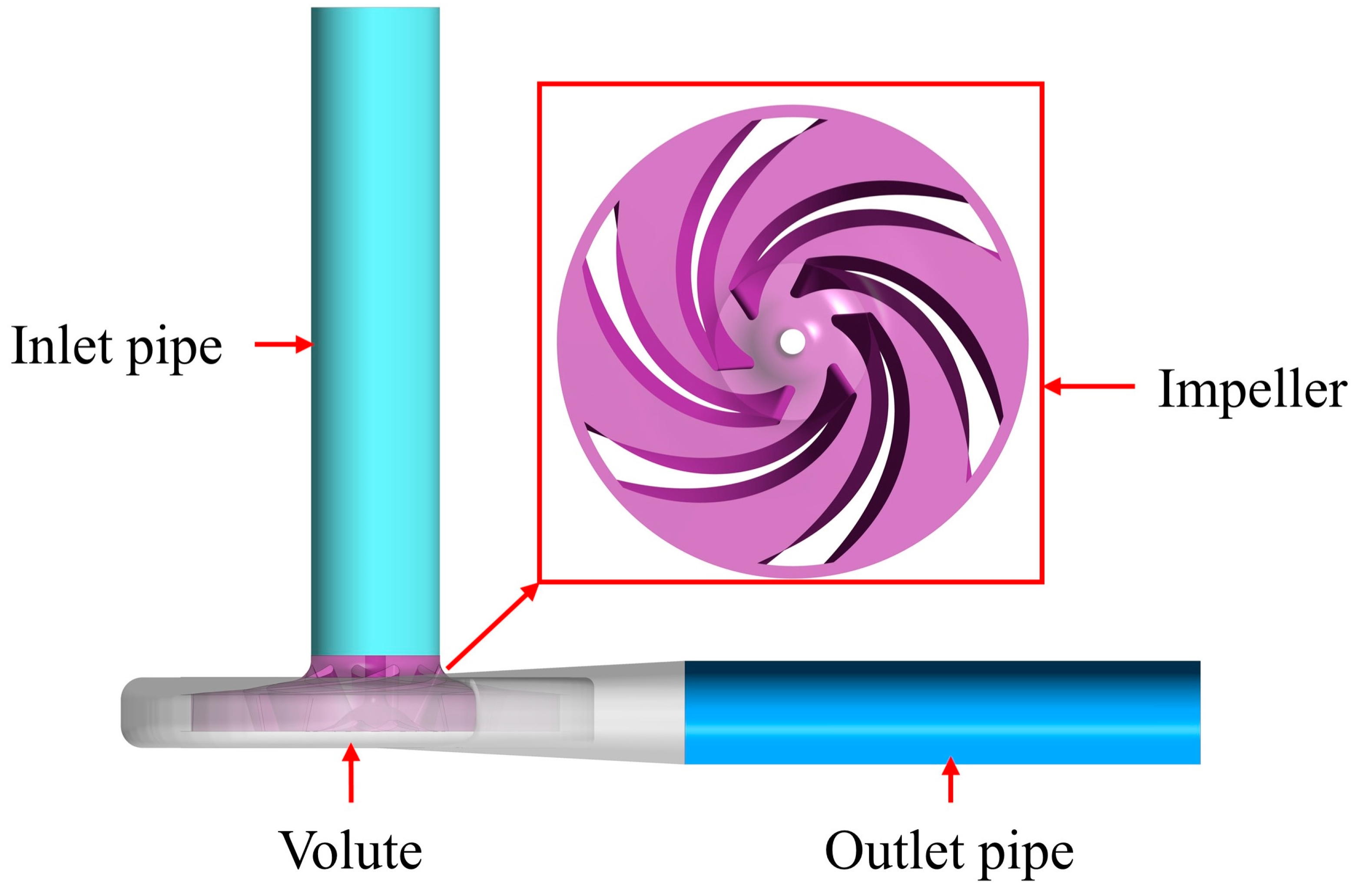
2.1. Marine Sediment Pump Model

The focus of the research is a marine sediment pump. The design flow rate Q_d is 160 m³/h (0.04444 m³/s), the design head H_d is 44 m, the rotational speed n is 1480 r/min, and the efficiency η_d is 68%. Therefore, the specific speed $n_s=\frac{3.65n\sqrt{Q_d}}{H^{\frac{3}{4}}}$ is about 67. The basic parameters of the marine sediment pump are depicted in

Table 1. The basic parameters of the marine sediment pump.

Parameter	Value	Parameter	Value
Impeller inlet diameter D1/mm	125	Blade outlet angle β2/°	27
Impeller outlet diameter D2/mm	358	Blade wrap angle φ/°	110
Impeller outlet width b2/mm	36	Volute base diameter D3/mm	378
Number of impeller blades Z	6	Volute inlet width b3/mm	68
Blade inlet angle β1/°	27	Volute outlet diameter D4/mm	100

, and the three-dimensional fluid domain is depicted in Figure 1.

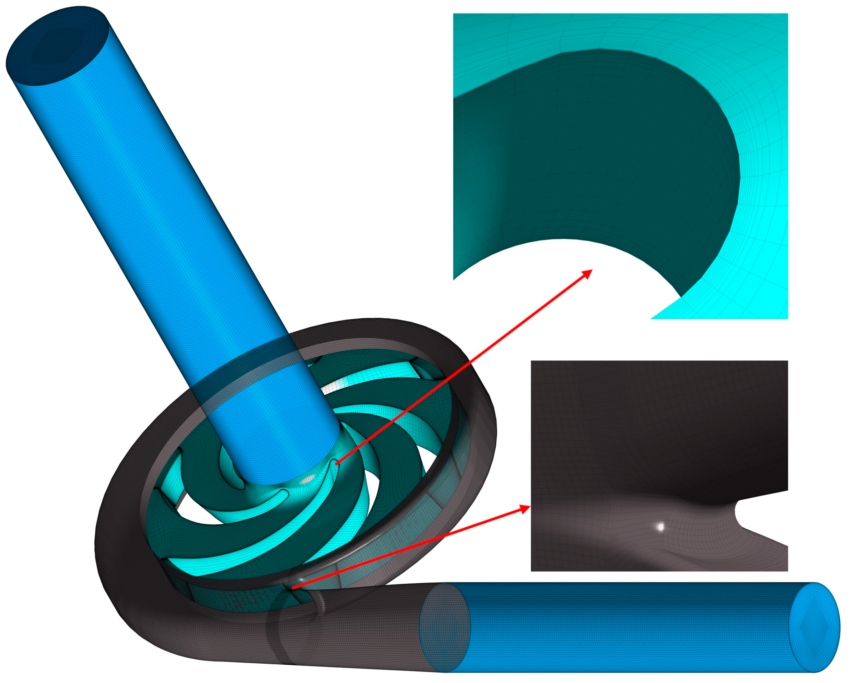
2.2. Mesh Independence Investigation

The overall mesh division of the calculation domain of the marine sediment pump is given in Figure 2. The four calculation domains are divided by hexahedral mesh cells, and the mesh near the key walls is refined. The overall mesh cell quality remains above 0.3, maintaining a mesh minimum corner angle exceeding 18°, while the y+ values along the wall remain below 20, which can fulfill the near-wall mesh configuration of the SST k-ω turbulence model [22]. Under the design conditions, the same boundary conditions are used to simulate the computational domain with five different mesh number schemes, and the head and efficiency are recorded. The specific data of the mesh-independent analysis of the marine sediment pump are shown in

Table 2. Mesh independence verification form.

Mesh Cells	Head (m)	Efficiency (%)
815,779	77.72	52.65
1,819,903	77.05	52.03
3,003,478	76.60	51.62
4,077,080	76.44	51.48
5,253,809	76.35	51.43

and Figure 3. In the case where the number of mesh cells exceeds 3,003,478, the efficiency and head fluctuation range are both less than 0.5%. Therefore, to save computing resources and improve computing speed, the 3,003,478 meshes are selected for subsequent research.

2.3. Numerical Method and Boundary Conditions

The marine sediment pump’s numerical simulation is carried out with the commercial software ANSYS CFX 2020R2. The medium is configured as clean water and the temperature is configured as 298 K. The inlet, volute, and outlet are configured as the stationary domain, while the impeller is configured as the rotating domain. The SST k-ω model is adopted as the turbulence model. The inlet boundary condition is specified using total pressure, and its value is 1 atm (with a reference pressure of 0 atm). Meanwhile, the outlet boundary condition is specified using mass flow, and its value is 44.44 kg·s⁻¹. The rated speed is set to 1.480 r/min. The approach applied at the rotor–stator interface is the transient frozen rotor approach. The simulations are considered converged upon achieving root-mean-square residuals consistently below 1.0 × 10⁻⁵.

2.4. Experimental and Numerical Calculation Verification

2.4.1. Error Analysis of Test Bench

To further verify the accuracy of the numerical calculation results, this study conducted an experimental study on the original model of the marine sediment pump. Furthermore, this study also analyzed the uncertainty index of each measurement parameter and the overall accuracy of the test bench [23]. In the test, pressure sensors were used to monitor the inlet and outlet pressures. The measurement deviation of the inlet and outlet pressure sensors are both ±0.5%. In addition, the measurement deviation of the turbine flowmeter is ±0.5%, the measurement deviation of the torque sensor is ±0.5% and the speed sensor measurement deviation is ±1.0%.

The pressure measurement deviation of the inlet pressure sensor and the outlet pressure sensor are both ±0.5% (D_P = ±0.5%). The monitoring points of the inlet pressure sensor and the outlet sensor are installed on the inlet and outlet water tanks, respectively, so the velocity heads at the inlet and outlet monitoring points can be ignored, which means D_D = 0. Therefore, the head deviation can be obtained using the following calculation:

$$D_{\mathrm{H}}=\sqrt[2]{{D_{\mathrm{P}}}^2+{D_{\mathrm{D}}}^2}=\pm 0.5\mathrm{\%}$$

(1)

The measurement deviation of the turbine flowmeter is ±0.5%, so the flow measurement error D_Q of the test system is ±0.5%.

The torque measurement deviation of the torque sensor is ±0.5% (D_M = ±0.5%). The measurement deviation of the speed sensor is ±0.1% (D_N = ±0.1%). Therefore, the shaft power measurement deviation of the test system can be calculated as follows:

$$D_{\mathrm{T}}=\sqrt[2]{{D_{\mathrm{M}}}^2+{D_{\mathrm{N}}}^2}=\pm 0.51\mathrm{\%}$$

(2)

According to the measurement deviation of the above measurement parameters, it is concluded that the head deviation D_H = ±0.5%, the flow deviation D_Q = ±0.5%, and the shaft power measurement deviation D_T = ±0.51%. Therefore, the total measurement error of the test system is calculated:

$$D_{\mathrm{S}}=\sqrt[2]{{D_{\mathrm{H}}}^2+{D_{\mathrm{Q}}}^2+{D_{\mathrm{T}}}^2}=\pm 0.872\mathrm{\%}$$

(3)

The total measurement deviation D_S of the test bench is ±0.872%, which shows that the deviation of the test system is within the allowable range of the study. Therefore, the experimental analysis in this paper can effectively verify the numerical calculation results.

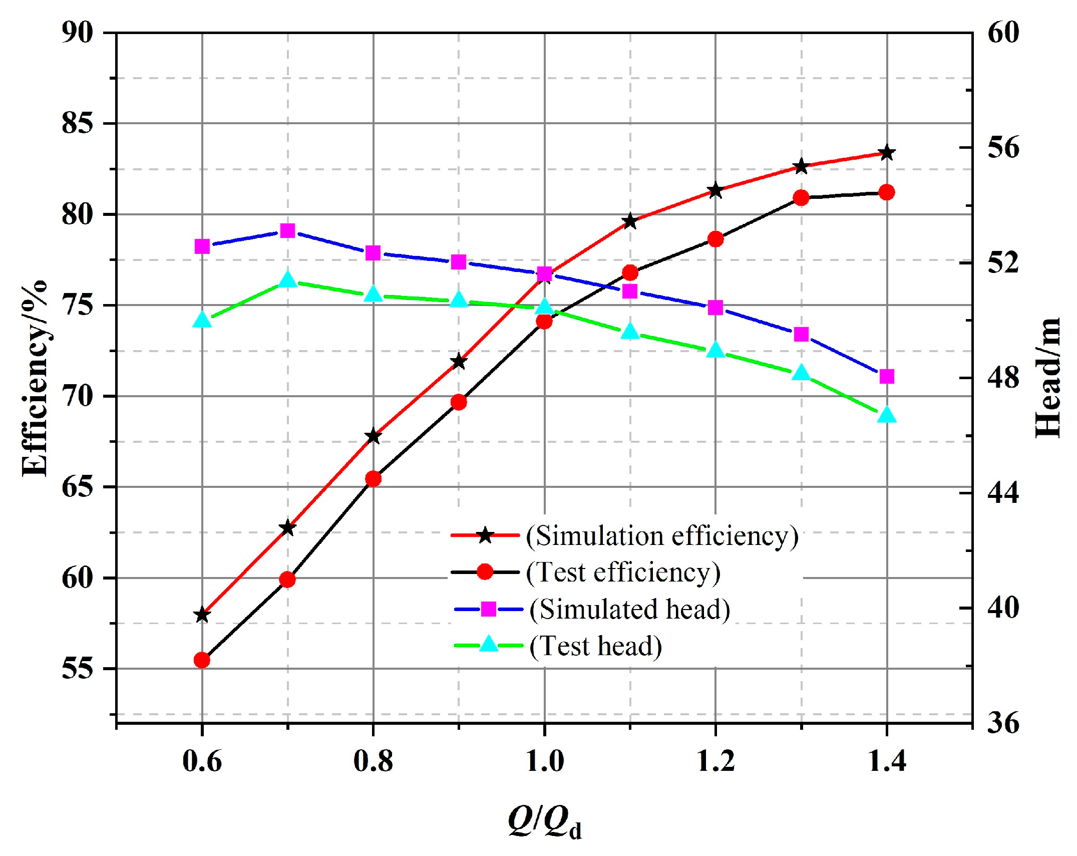
2.4.2. Comparison of Numerical Calculations and Experimental Results

The comparison of the external characteristics between the test and the simulation results is presented in Figure 4, and the marine sediment pump test bench is presented in Figure 5. As indicated in Figure 4, there is a strong agreement between the simulation and test results. The efficiency difference at the design flow rate is 2.48%, accompanied by a relative error of 3.35%. The head difference is 1.2 m, and the relative error is 2.38%. These errors are all within the reasonable range, which verifies the exactness of the numerical simulation.

3. Analysis of Response Surface Optimization

In this study, the target variable y is the efficiency of the marine sediment pump, while Z (the number of blades), β₁ (blade inlet angle), β₂ (blade outlet angle), and φ (blade wrap angle) are considered as the design variables.

Table 3. Original impeller design parameters.

Z (Number)	β1 (°)	β2 (°)	φ (°)
6	27	27	110

presents the original impeller design parameters for the marine sediment pump.

3.1. Response Surface Optimization Method

As illustrated in

Table 4. The range of values of design parameters.

Variable	Z (Number)	β1 (°)	β2 (°)	φ (°)
Lower limit	6	22	17	130
Upper limit	8	32	27	160

, based on the marine sediment pump model’s design parameters, the value ranges for the four design parameters are established.

By employing the response surface optimization method, the four design parameters are sampled within the range of values. The sampling results are modeled based on CFTurbo, and the model is numerically simulated by ANSYS CFX. Finally, the efficiency values corresponding to each model are obtained, and the specific results are shown in

Table 5. Test schemes.

Standard Sequence	Running Program	Factor1: Z x1	Factor2: β1 x2	Factor3: β2 x3	Factor4: φ x4	Response: Efficiency y
4	1	8	32	17	130	81.94
16	2	8	32	27	160	79.59
19	3	7	22	22	145	82.12
17	4	6	27	22	145	81.74
11	5	6	32	17	160	82.93
10	6	8	22	17	160	81.86
14	7	8	22	27	160	80.25
2	8	8	22	17	130	81.65
24	9	7	27	22	160	82.40
1	10	6	22	17	130	81.82
20	11	7	32	22	145	82.11
23	12	7	27	22	130	81.67
18	13	8	27	22	145	81.63
8	14	8	32	27	130	80.68
25	15	7	27	22	145	82.23
6	16	8	22	27	130	80.95
13	17	6	22	27	160	81.47
7	18	6	32	27	130	80.74
3	19	6	32	17	130	81.83
22	20	7	27	27	145	81.19
9	21	6	22	17	160	82.61
12	22	8	32	17	160	81.39
21	23	7	27	17	145	82.70
5	24	6	22	27	130	80.81
15	25	6	32	27	160	81.25

.

3.2. Analysis of Variance and Response Regression Model Analysis

Variance is a mathematical quantity that measures the extent of dispersion between a random variable and its expected value. Considering the two-factor interaction, Minitab software 17 is adopted to conduct variance analysis on the response variable efficiency y, and the outcomes are displayed in

Table 6. Variance analysis table.

Variance Analysis
Source	Degrees of Freedom	Adj SS	Adj MS	F Value	p Value
Model	14	14.2030	1.01450	19.70	0.000
Linear	4	9.4905	2.37263	46.08	0.000
Z	1	1.5371	1.53709	29.85	0.000
β1	1	0.0648	0.06480	1.26	0.288
β2	1	7.7356	7.73556	150.24	0.000
φ	1	0.1531	0.15309	2.97	0.115
Square	4	2.4607	0.61519	11.95	0.001
Z × Z	1	0.5374	0.53744	10.44	0.009
β1 × β1	1	0.0022	0.00220	0.04	0.840
β2 × β2	1	0.1012	0.10124	1.97	0.191
φ × φ	1	0.0305	0.03047	0.59	0.460
Two-factor interaction	6	2.2517	0.37528	7.29	0.003
Z × β1	1	0.0827	0.08266	1.61	0.234
Z × β2	1	0.0127	0.01266	0.25	0.631
Z × φ	1	1.6835	1.68351	32.70	0.000
β1 × β2	1	0.1173	0.11731	2.28	0.162
β1 × φ	1	0.0613	0.06126	1.19	0.301
β2 × φ	1	0.2943	0.29431	5.72	0.038
Deviation	10	0.5149	0.05149
Total	24	14.7179

.

In the variance analysis of the response surface regression model, the p value can be used to judge whether each item has a significant impact on the response variable y. Considering the accuracy and reliability of the response surface regression model variance analysis, a confidence level of 95% was selected to determine the relationship between the design variables and the response variable y. If p > 0.05, it means the impact of this item on y is not significant, and this item should be deleted and recalculated. If p ≤ 0.05, it signifies that the item holds a significant influence on variable y. However, if p ≤ 0.01, it indicates a notably pronounced impact of this item on variable y, underscoring its heightened importance in influencing y.

Table 6 shows that the p value of the model is zero, unequivocally establishing the model’s statistical significance. Additionally, the sources Z, β₂, Z × Z, Z × φ, and β₂ × φ are all significant impact factors because their p values are less than 0.05. And the parameters β₁, φ, β₁ × β₁, β₂ × β₂, φ × φ, Z × β₁, Z × β₂, β₁ × β_2, and β₁ × φ are all non-significant impact factors because their p values are greater than 0.05. However, due to the significant interaction between the main effect φ and the main effects Z and β₂, this causes the significance of φ to be affected. The existence of this interaction increases the uncertainty of φ in the response surface model, making φ become significant in the new model, which removes insignificant factors. Therefore, to account for the interaction effects of the main effects, this study chose to adopt a response surface analysis design with a hierarchical structure, in which all lower-order terms that make up the higher-order terms are considered in the model. Therefore, φ is reconsidered as a significant factor.

After removing insignificant factors, the main effect diagram of the influence trend of a single factor on efficiency is shown in Figure 6. This suggests that the connection between Z and efficiency follows a quadratic pattern, while the correlation between β₂ and efficiency is negative. Furthermore, the association between φ and efficiency displays a positive correlation.

Based on statistical analysis and parameter fitting theory in mathematical statistics, the approximate functional relationship between the independent variable and the response variable can be obtained and expressed as a functional formula between the response variable y and the independent variables (x₁, x₂……):

$$y=f\left(x_1,x_2\cdots \right)$$

(4)

When the number of independent variables is 1, the response surface graph is a straight line. In engineering practice, the number of independent variables is generally multiple, and the response surface graph is a spatial surface. The response surface function, that is, the regression equation, has the following form:

$$y=a_1+a_2\sum _1^{\mathrm{n}} x_{\mathrm{i}}+a_3\sum _1^{\mathrm{n}} x_{\mathrm{i}}^2+a_4\sum _1^{\mathrm{n}} x_{\mathrm{i}}{x}_{\mathrm{j}}$$

(5)

In the formula, $x_{\mathrm{i}}$is the linear term independent variable; $x_{\mathrm{i}}^2$ is the quadratic term independent variable; and $x_{\mathrm{i}}{x}_{\mathrm{j}}$ is the interaction term independent variable.

Therefore, after eliminating factors that have no significant impact on efficiency, the response surface regression model of the marine sediment pump efficiency is obtained:

$$\begin{gathered} \mathsf{\eta }=25.88+12.13Z+0.131{\beta }_2+0.1973\phi \\ -0.663Z\ast Z-0.2163\mathrm{Z}\ast \phi -0.001808{\beta }_2\ast \phi \end{gathered}$$

(6)

Substituting the original parameters of the marine sediment pump impeller into the response surface regression equation, the predicted value of the pump efficiency is 80.39%, and the deviation from the simulated efficiency is less than 5%, which meets the requirements.

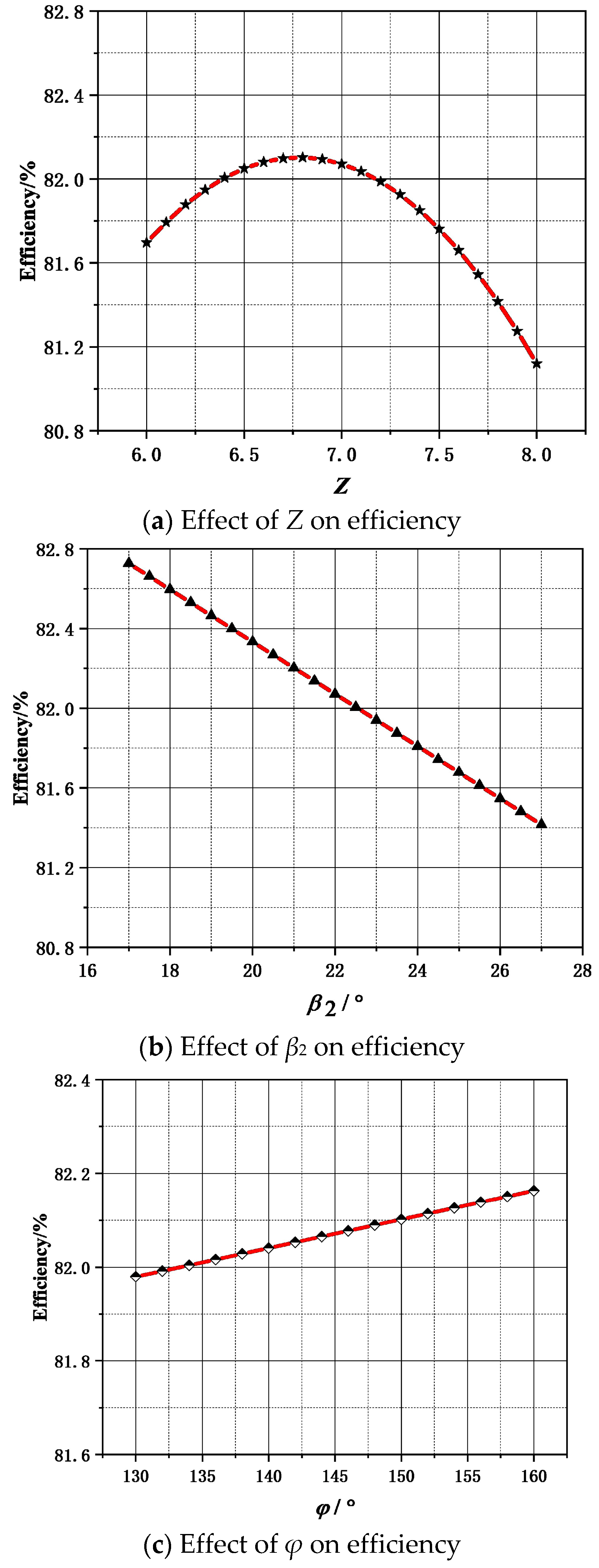
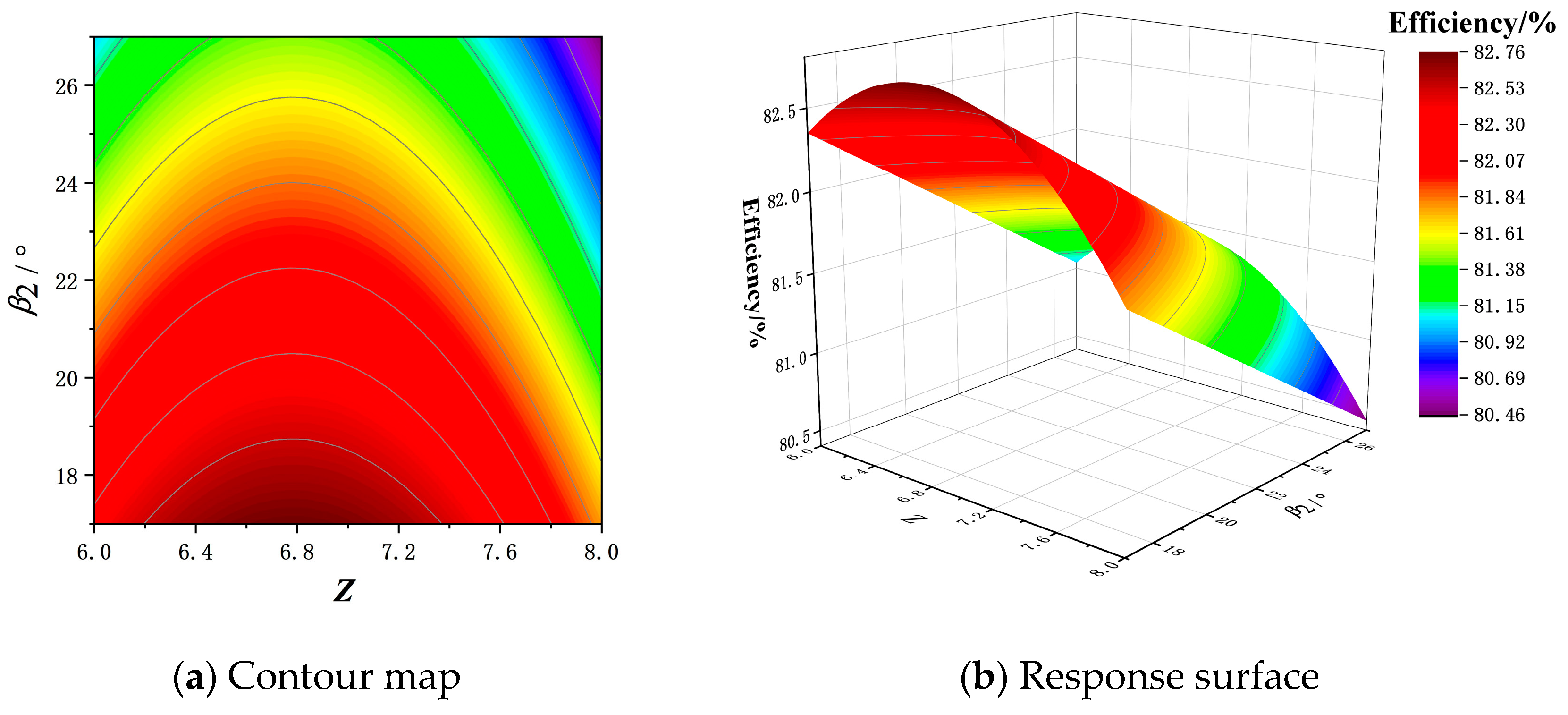
3.3. Analysis of Response Surface Diagram and Contour Diagram

Figure 7, Figure 8 and Figure 9 depict the correlation between the efficiency η of the response variable and the three design variables. Figure 6a is the contour map and Figure 6b is a response surface map. As shown in Figure 6, when Z is constant, β₂ is negatively correlated with the efficiency. When β₂ is constant, the efficiency initially rises and subsequently decreases as Z increases. As depicted in Figure 7, when Z is less than 7, φ is positively correlated with efficiency, and when Z is larger than 7, φ is negatively correlated with efficiency. While maintaining a constant value for φ, the efficiency exhibits an upward trend followed by a downturn as the Z increases.

As shown in Figure 8, when β₂ remains constant, there is a positive correlation between φ and efficiency. Conversely, when φ is constant, β₂ is negatively correlated with efficiency in the range of 17°–27°. By analyzing the two-factor interaction diagram, both Z and β₂ exert a more pronounced influence on efficiency, while the effect of φ on efficiency is relatively insignificant. When Z and β₂ are within a specific range, the efficiency has an extreme value, which aligns with the findings presented in Table 6.

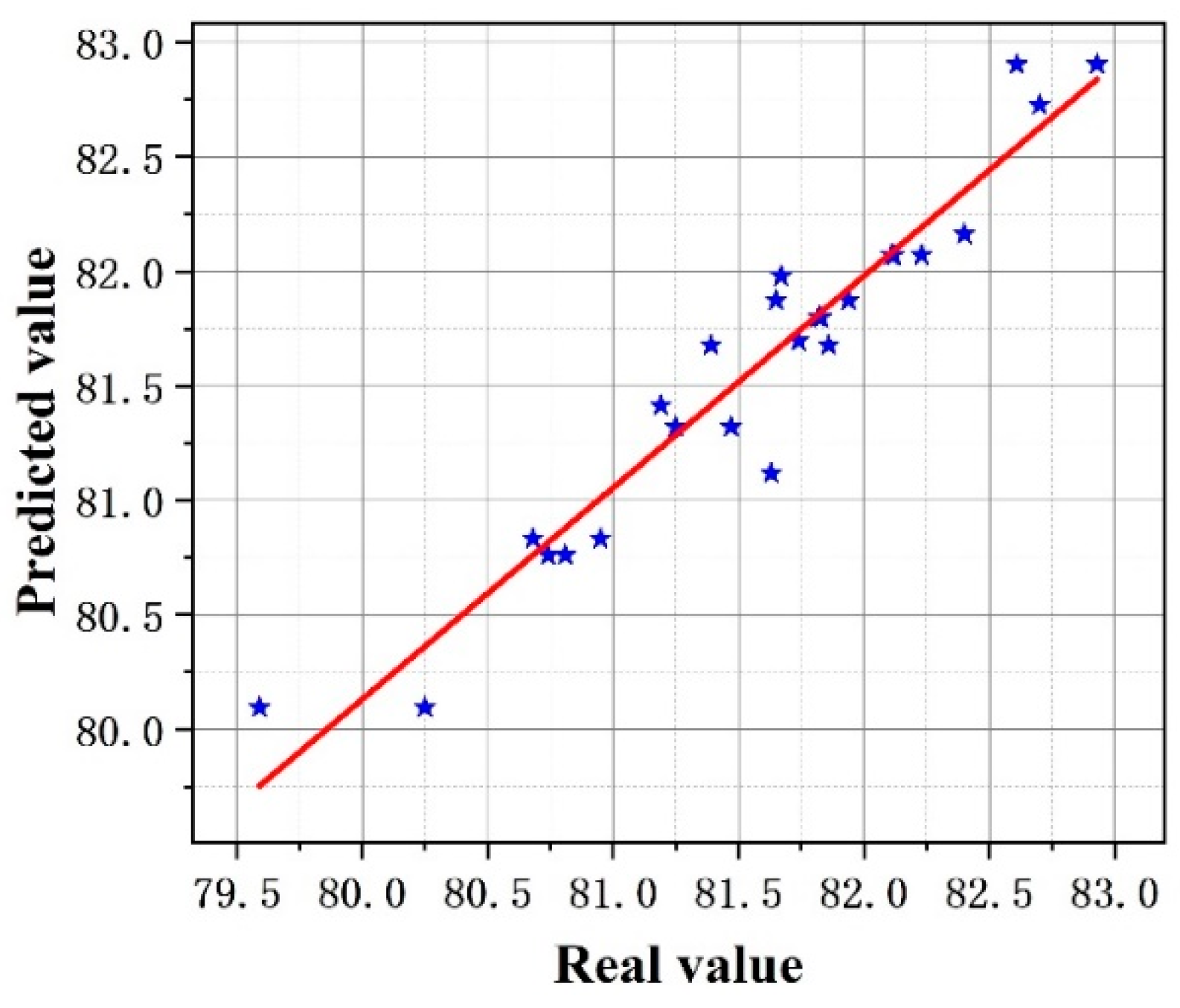
3.4. Analysis of the Prediction Model

In this investigation, the predictive model for the marine sediment pump is obtained by utilizing the response surface optimization methodology. The accuracy of the prediction model is assessed using the correlation coefficient R² error analysis approach, employing the following formula:

$$R^2=1-\frac{\sum _{\mathrm{i}=1}^n {\left(\widehat{y}-y_{\mathrm{i}}\right)}^2}{\sum _{\mathrm{i}=1}^n {\left(y_{\mathrm{i}}-\overline{y}\right)}^2}$$

(7)

where $\widehat{y}$ is the predicted value of the response surface, $y_{\mathrm{i}}$ is the simulated value of the numerical calculation, and $\overline{y}$ is the average value of the response surface.

In Figure 10, the correlation coefficient of the marine sediment pump efficiency is calculated to be 0.9252. This high correlation coefficient indicates that the response surface optimization is effective at accurately establishing the functional relationship between the efficiency η and the design variables. Based on the optimization analysis, the predicted optimal values for the optimized impeller model are within a reasonable range: Z is 6, β₁ is 32°, β₂ is 17°, and φ is 160°. These optimization measures are anticipated to increase the efficiency of the marine sediment pump.

Figure 11 illustrates the contrasting impeller blade structures between the original model and the optimized model, while Figure 12 showcases the external characteristic curves. The efficiency of the optimized model has been significantly enhanced, and the head is reduced while still meeting the design conditions. The efficiency of the optimized model is elevated by 6.33% under the design condition, a 2% increase in efficiency under the overload flow conditions, and increased by more than 8% under the partial load flow conditions.

4. Analysis of the Internal Flow Field

Unsteady numerical calculation is performed under five flow conditions (0.6Q_d, 0.8Q_d, 1.0Q_d, 1.2Q_d, and 1.4Q_d). The result of 10 rotations of the impeller is calculated, and the time step is set to 0.000337838 s (every 3° of rotation of the impeller), with a convergence accuracy set to 10⁻⁵. Figure 13 illustrates the arrangement of monitoring points on the impeller. The arrangement of monitoring points on the volute is depicted in Figure 14. During the entire calculation process, physical parameters such as head, efficiency, and mass flow rates are all monitored. The configuration conditions remain consistent across different flow scenarios, except for varying flow rates.

4.1. Analysis of Flow Field

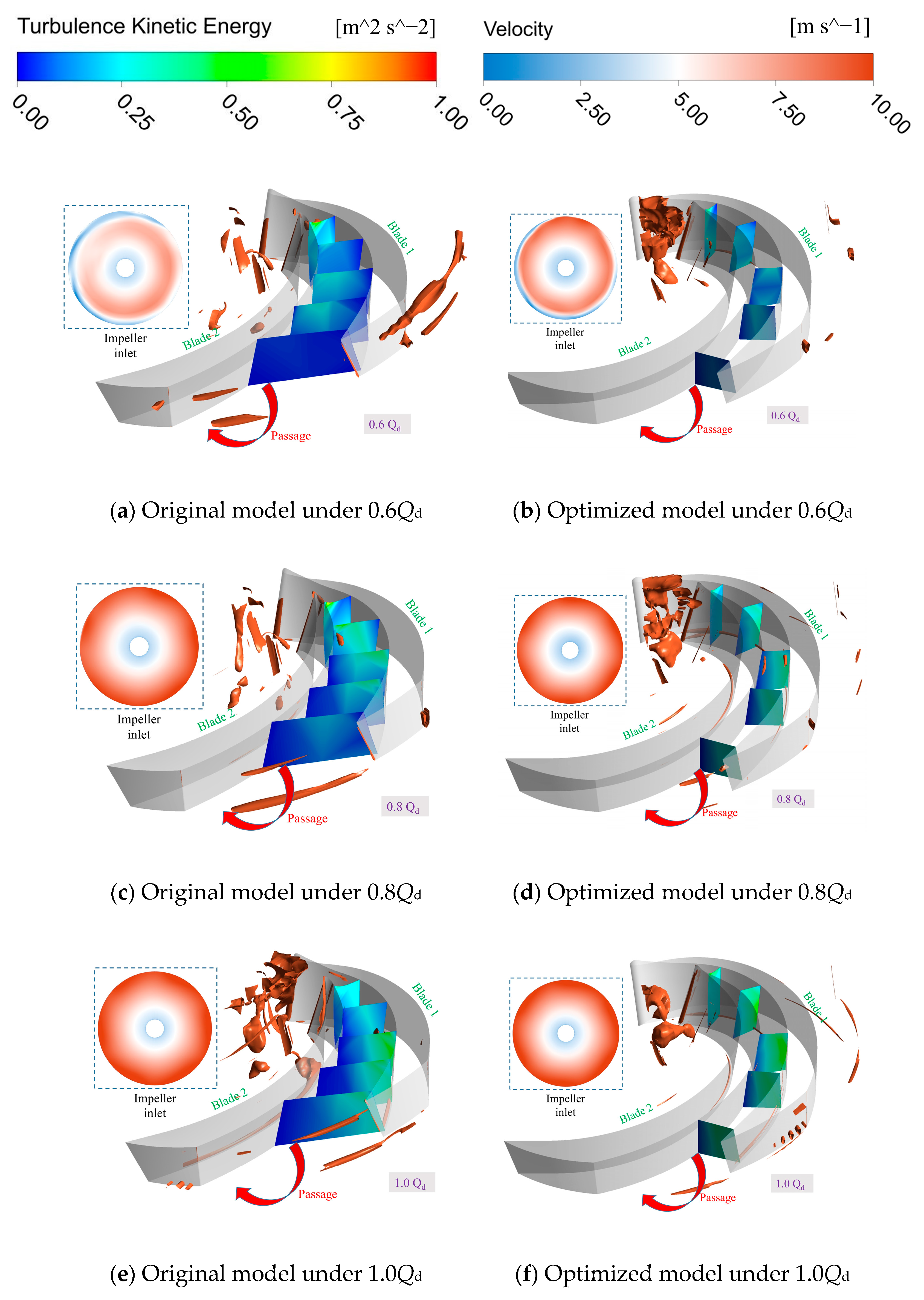
4.1.1. Analysis of Impeller Internal Flow

Figure 15 illustrates variations in impeller inlet velocity and distribution of vortex and turbulent kinetic energy (TKE) across a single impeller flow channel at five various flow conditions (Q/Q_d = 0.6, 0.8, 1.0, 1.2, and 1.4). The sections are categorized as (1) through (5) in sequence from the impeller flow channel’s inlet to its outlet. This arrangement facilitates the explanation of variations in the TKE distribution across the impeller flow channels. Under varying flow conditions, the highest TKE is generated within section (1). As the flow rate increases, the TKE on the pressure surface of the blade gradually diminishes, while the TKE on the blade suction surface gradually increases. Figure 15 illustrates that the velocity distribution at the impeller inlet remains nearly identical between the original model and the optimized model. The distribution of TKE in the impeller flow channel of the original model is extremely uneven under five flow conditions, while the optimized model only has an uneven TKE distribution under partial load flow conditions. Under both the design and overload flow conditions, the TKE distribution within the optimized model’s flow channel becomes more uniform, and a substantial reduction in large-area vortices is observed. This signifies a notable enhancement in the outlet velocity of the optimized model, leading to a more even distribution of flow velocities.

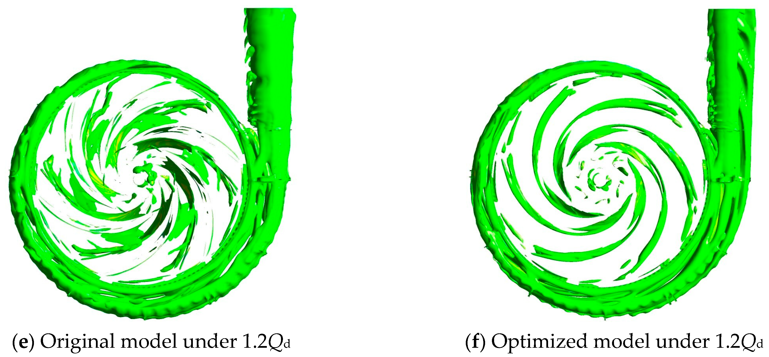
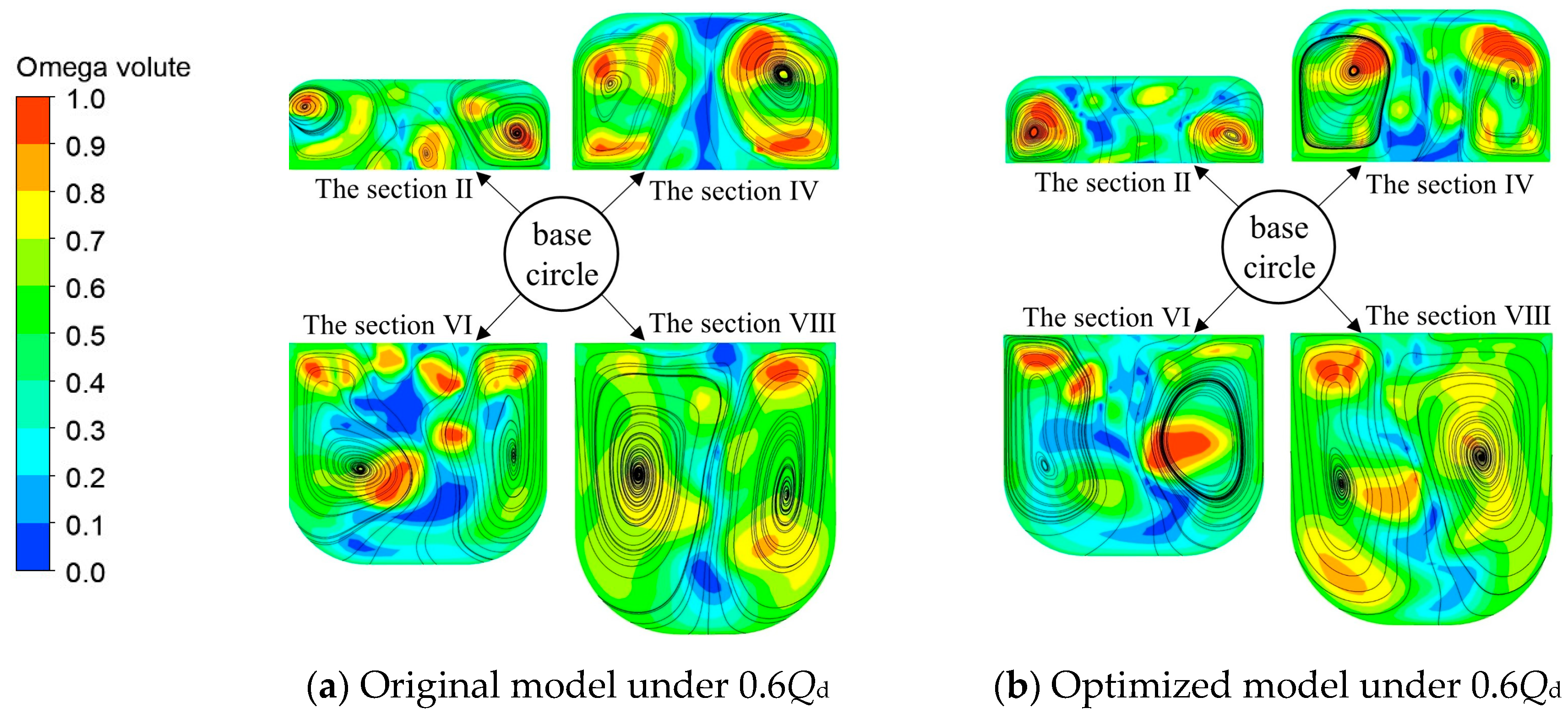
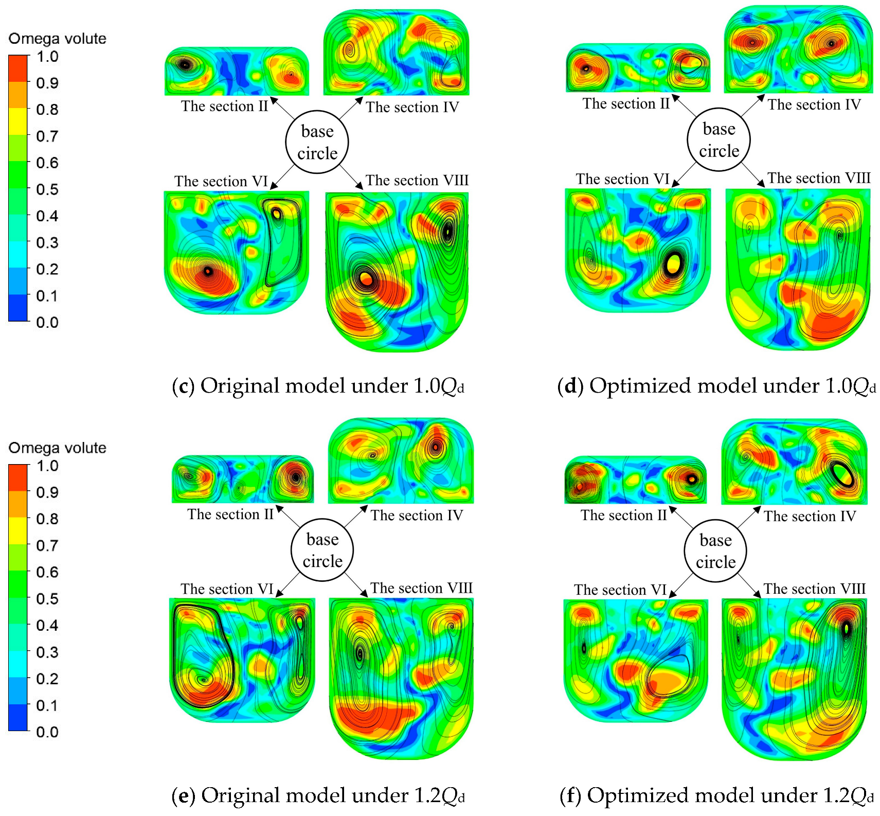
4.1.2. Analysis of Omega Vortex Identification Results

The formation and evolution of vortices are intricately linked to the dynamic and unsteady flow characteristics of marine sediment pumps [24,25]. Accurately capturing the distribution of vortex structures holds immense significance for ensuring the stable operation of fluid machinery. Regularized helicity, maximum vorticity, Q criterion, and λ₂ criterion vortex identification methods have been applied to a certain extent. However, traditional vortex identification methods exhibit noticeable shortcomings, and the regularized helicity and maximum vorticity methods cannot represent the strength of eddies well. Both the Q criterion and λ₂ criterion are highly sensitive to the choice of threshold values, and an unreasonable selection of the threshold will lead to incomplete vortex identification [26,27]. Therefore, the Omega vortex identification method was proposed by Liu et al. [28,29]. This method offers a well-defined threshold selection criterion, resulting in significantly improved vortex identification performance compared to traditional methods. Zhang et al. [30] demonstrated the applicability of the vortex identification method to water pumps.

In the Omega vortex identification method, the vorticity ω is partitioned into a rotating part A and a non-rotating part B:

$$\mathit{\omega }=\mathit{A}+\mathit{B}$$

(8)

The parameter R is used to represent the ratio of the vorticity of the rotating part to the total vorticity, and the formula is:

$$R=\frac{\parallel \mathit{B}{\parallel }_F^2}{\parallel \mathit{A}{\parallel }_F^2+\parallel \mathit{B}{\parallel }_F^2+\epsilon }$$

(9)

where$\epsilon$ is a small positive value added to avoid division by zero in the denominator.

R is the concentration of vorticity, and its value range is 0 ≤ R ≤ 1. If R is 0, it means that there is only shear force in the flow field, and there is no vortex. If R > 0.5, it means that the antisymmetric tensor B is higher than the symmetric tensor A, so it can be used as the basis for vorticity discrimination. If R = 1, it means that the fluid rotates rigidly. Zhao et al. [31] confirmed that the largest area vortex appears when the threshold R is selected as 0.52, and the threshold is the optimal solution.

Under various flow conditions, the distribution of vortex identification using the Omega method are illustrated in Figure 16. The main vortex characteristics of the pump’s internal flow field can be effectively captured by the Omega vortex identification method. Under different flow conditions, the vortices of the optimized model and the original model exhibit the same variation regulation. Under partial load flow conditions, the vortex appears to be highly disordered in the flow field. A multitude of small-scale vortices emerge at the impeller flow channel’s inlet and the volute, whereas a continuous vortex is discernible at the blade’s suction surface. This observation implies that fluid flow within these regions is comparatively unstable. With an increase in the flow rate, the vortex within the impeller flow channel decreases, resulting in a more stabilized flow field, which aligns with the behavior of the velocity streamline. The vortex in the volute undergoes continuous evolution and diffusion with the fluid’s movement, ultimately dissipating in the volute diffusion section. In contrast to the original model, the optimized model exhibits fewer vortices under different flow conditions. This suggests that the optimized model provides better flow conditions compared to the original model.

Figure 17 illustrates the distribution of Omega vortices and streamlines at sections II, IV, VI, and VIII in the volute under various flow conditions (Q/Q_d = 0.6, 1.0 and 1.2). And the sections II, IV, VI, and VIII are shown in Figure 14. The actual operation of the pump is influenced by various factors such as wall conditions and flow rates, and the regions with higher Omega values align more closely with the vortex distribution. The distribution of high-Omega-value areas of the original model appears to be relatively scattered under partial load flow conditions, with numerous vortices observed in section II. In contrast, the high-Omega-value area of the optimized model is more concentrated, and the streamlined distribution is more regular, primarily concentrated on both sides of the volute section. Under overload flow conditions, the optimized model also experiences a reduction in the high-Omega-value area, and the effect is remarkable in the VI and VIII sections. Under the design conditions, the distribution of the high-Omega-value area is more regular compared to the partial load flow conditions. In each section, the optimized model exhibits a reduction in the high-Omega-value area, with the most significant effect observed in section VIII, which indicates a significant improvement in the fluid flow characteristics of the optimized model.

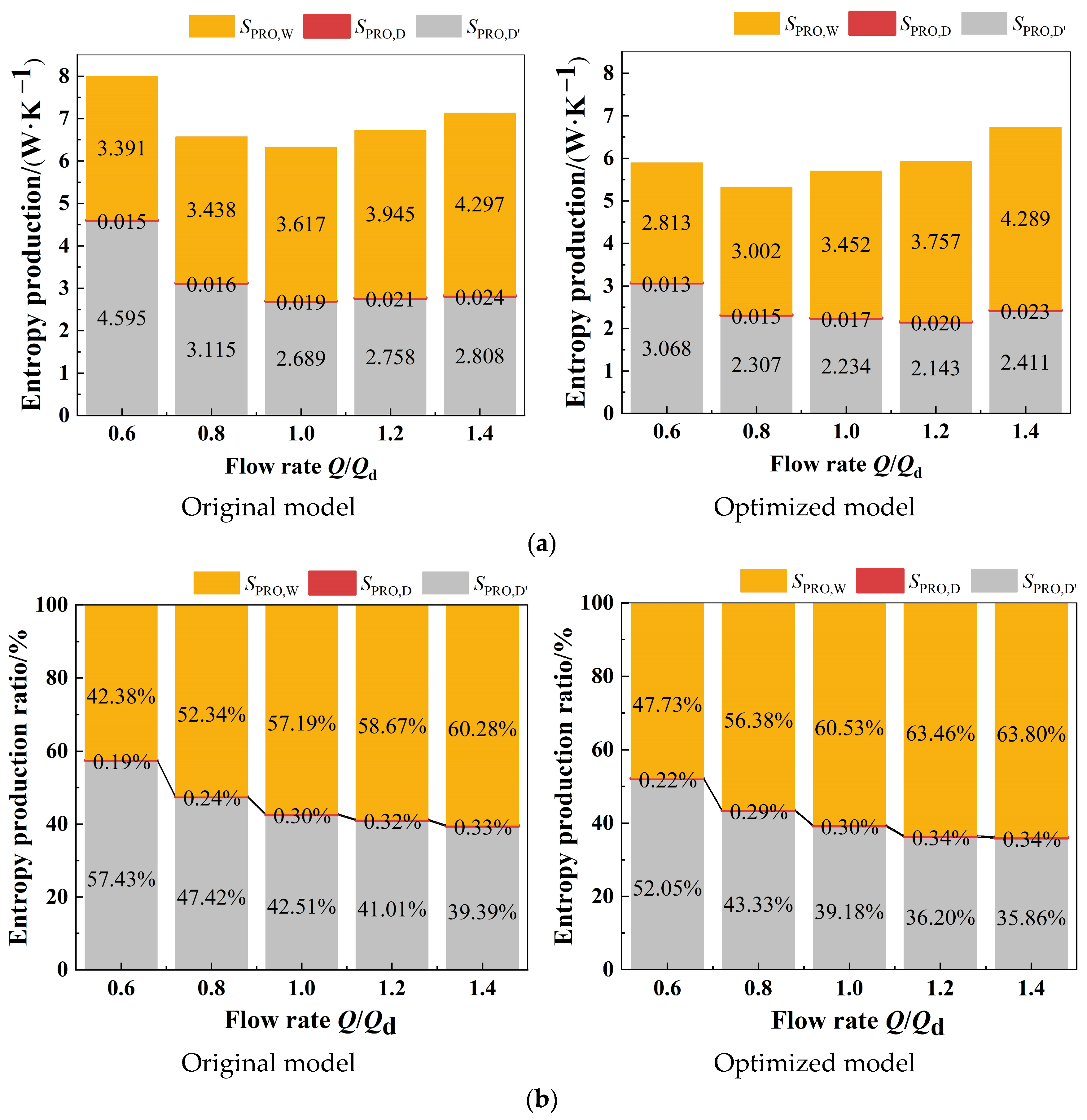
4.2. Analysis of Entropy Production

Rotating machinery will consistently convert a portion of mechanical energy into internal energy during operation, leading to irreversible energy dissipation [32,33]. Therefore, entropy production, as a state parameter for evaluating energy changes, has gained widespread application in the field of energy dissipation in rotating machinery. In this study, it is assumed that temperature remains constant. The transport equation for entropy is as follows:

$$\rho \left(\frac{\partial s}{\partial t}+u\frac{\partial s}{\partial x}+v\frac{\partial s}{\partial y}+w\frac{\partial s}{\partial z}\right)=-\mathrm{d}\mathrm{i}\mathrm{v}\left(\frac{\mathbf{q}}{T}\right)+\frac{\Phi }{T}+\frac{{\Phi }_{\theta }}{T^2}$$

(10)

In Equation (10), there are two sources of entropy generation: viscous dissipation and heat transfer. Under the assumption of constant temperature, the entropy production occurs only in viscous dissipation, as depicted in the following Equation (11):

$$S=S_D=\frac{\Phi }{T}$$

(11)

Time-averaged motion and velocity fluctuations are the main components of entropy production within the pump.

Entropy production within the pump is primarily attributed to time-averaged motion and velocity fluctuations. Therefore, the calculation for S is as follows:

$$S=S_{\mathrm{P}\mathrm{R}\mathrm{O},\mathrm{D}}+S_{\mathrm{P}\mathrm{R}\mathrm{O},\mathrm{D}\prime }$$

(12)

The computation for the time-averaged motion is conducted in the following manner:

$$\begin{array}{cc}{S}_D^{‴}=& 2\frac{{\mu }_{\mathrm{e}\mathrm{f}\mathrm{f}}}{T}\left[{\left(\frac{\partial \overline{v_x}}{\partial x}\right)}^2+{\left(\frac{\partial \overline{v_y}}{\partial y}\right)}^2+{\left(\frac{\partial \overline{v_z}}{\partial z}\right)}^2\right]\hfill \\ & +\frac{{\mu }_{\mathrm{e}\mathrm{f}\mathrm{f}}}{T}\left[{\left(\frac{\partial \overline{v_y}}{\partial x}+\frac{\partial \overline{v_x}}{\partial y}\right)}^2+{\left(\frac{\partial \overline{v_z}}{\partial x}+\frac{\partial \overline{v_x}}{\partial z}\right)}^2+{\left(\frac{\partial \overline{v_y}}{\partial z}+\frac{\partial \overline{v_z}}{\partial y}\right)}^2\right]\hfill \end{array}$$

(13)

The calculation for the turbulent dissipation is performed as follows:

$$\begin{array}{cc}{S}_{D^{\prime }}^{‴}=& 2\frac{{\mu }_{\mathrm{e}\mathrm{f}\mathrm{f}}}{T}\left[{\left(\frac{\partial v_x^{\prime }}{\partial x}\right)}^2+{\left(\frac{\partial v_y^{\prime }}{\partial y}\right)}^2+{\left(\frac{\partial v_z^{\prime }}{\partial z}\right)}^2\right]\hfill \\ & +\frac{{\mu }_{\mathrm{e}\mathrm{f}\mathrm{f}}}{T}\left[{\left(\frac{\partial v_y^{\prime }}{\partial x}+\frac{\partial v_x^{\prime }}{\partial y}\right)}^2+{\left(\frac{\partial v_z^{\prime }}{\partial x}+\frac{\partial v_x^{\prime }}{\partial z}\right)}^2+{\left(\frac{\partial v_y^{\prime }}{\partial z}+\frac{\partial v_z^{\prime }}{\partial y}\right)}^2\right]\hfill \end{array}$$

(14)

Since the turbulence model in this simulation uses the SST k-ω model, direct extraction of the velocity fluctuation component is not feasible. According to the literature [34,35], the entropy production rate associated with turbulent dissipation can be estimated using the following formula:

$$S_{D^{\prime }}^{‴}=\beta \frac{\rho \omega k}{T}$$

(15)

where β = 0.09.

Therefore, integrating the above equation, the entropy production is obtained:

$$S_{\mathrm{P}\mathrm{R}\mathrm{O},\mathrm{D}}={\int }_V S_D^{‴}dV$$

(16)

$$S_{\mathrm{P}\mathrm{R}\mathrm{O},\mathrm{D}\prime }={\int }_V S_{D^{\prime }}^{‴}dV$$

(17)

The RANS model cannot reasonably deal with strong wall effects, resulting in large errors in the near-wall region. Therefore, the entropy production near the wall surface is calculated using Equation (16).

$$S_{\mathrm{P}\mathrm{R}\mathrm{O},\mathrm{W}}={\int }_A \frac{\mathit{\tau }\cdot \mathbf{v}}{T}dA$$

(18)

where A is the area (m²), $\tau$ is the shear stress (Pa), and $\mathit{v}$ is the mesh velocity closest to the wall (m/s).

The entropy production of the pump can be represented by Equation (17), and the energy loss resulting from entropy production can be described as per Equation (18).

$$S_{\mathrm{P}}=S_{\mathrm{P}\mathrm{R}\mathrm{O},\mathrm{D}}+S_{\mathrm{P}\mathrm{R}\mathrm{O},\mathrm{D}\prime }+S_{\mathrm{P}\mathrm{R}\mathrm{O},\mathrm{W}}$$

(19)

$$E_{\mathrm{P}}=S_{\mathrm{P}}\cdot T=T\left(S_{\mathrm{P}\mathrm{R}\mathrm{O},\mathrm{D}}+S_{\mathrm{P}\mathrm{R}\mathrm{O},\mathrm{D}\prime }+S_{\mathrm{P}\mathrm{R}\mathrm{O},\mathrm{W}}\right)$$

(20)

Figure 18 depicts the distribution characteristics of the three types of entropy production under different flow conditions (Q/Q_d = 0.6, 0.8, 1.0, 1.2, and 1.4). Both the wall entropy production ($S_{\mathrm{P}\mathrm{R}\mathrm{O},\mathrm{W}}$) and the direct entropy production ($S_{\mathrm{P}\mathrm{R}\mathrm{O},\mathrm{D}}$) of both the original model and the optimized model exhibited an initial increase followed by a decrease with the escalation in the flow rate. In contrast, the turbulent entropy production ($S_{\mathrm{P}\mathrm{R}\mathrm{O},\mathrm{D}\prime }$) has consistently decreased with the rise in flow rate. Comparing the three types of entropy production values of the optimized and original models, it becomes evident that across diverse flow conditions, the wall entropy production${(S}_{\mathrm{P}\mathrm{R}\mathrm{O},\mathrm{W}})$, the turbulent entropy production ($S_{\mathrm{P}\mathrm{R}\mathrm{O},\mathrm{D}\prime }$) and the direct entropy production ($S_{\mathrm{P}\mathrm{R}\mathrm{O},\mathrm{D}}$) of the optimized model have been decreased. Among them, the wall entropy production ($S_{\mathrm{P}\mathrm{R}\mathrm{O},\mathrm{W}}$) ratio and the turbulent entropy production $\left(S_{\mathrm{P}\mathrm{R}\mathrm{O},{\mathrm{D}}^{\prime }}\right)$ ratio are larger, while the direct entropy production ($S_{\mathrm{P}\mathrm{R}\mathrm{O},\mathrm{D}}$) ratio does not exceed 1%. Furthermore, the data from both the optimized model and the original model reveal a notable increase in the wall entropy production ($S_{\mathrm{P}\mathrm{R}\mathrm{O},\mathrm{W}}$) ratio as the flow rate rises, while the direct entropy production ($S_{\mathrm{P}\mathrm{R}\mathrm{O},\mathrm{D}}$) ratio experiences a slight increment. But the turbulent entropy production ($S_{\mathrm{P}\mathrm{R}\mathrm{O},\mathrm{D}\prime }$) ratio decreased significantly.

Under different flow conditions, the distribution characteristics of total entropy production in the marine sediment pump are depicted in Figure 19. Both the original and optimized models exhibit a consistent trend in the entropy production distribution across various flow parts. The highest-entropy production occurs at the volute, followed by the impeller, and then the outlet. Additionally, in both models, the lowest entropy production is observed at the inlet. The entropy production at the inlet of both the original and optimized models is nearly identical, owing to consistent inflow conditions between the two models. Furthermore, the entropy production within the volute and outlet of the optimized model is lower compared to the original model. Within the impeller, under partial load flow conditions, the entropy production of the optimized model is lower than the original model. However, under the overload flow conditions and the design condition, the entropy production of the optimized model’s impeller surpasses the original model. This phenomenon primarily stems from the augmentation of the impeller’s wrap angle and blade curvature, resulting in a reduction in turbulence and direct entropy production. These structural alterations have also led to an increase in wall entropy production. And as the flow rate increases, the increased rate of wall entropy production is greater than the decline rate of local entropy production. The entropy production ratio of the original model and the optimized model show the same changing trend as the flow rate gradually increases. In the process of gradually increasing the flow rate, the entropy production ratio of the inlet and the outlet does not change much. Among them, the entropy production ratio of the outlet is gradually increasing, while the entropy production ratio of the inlet first decreases and then increases. In the impeller, with the increase in the flow rate, the entropy production ratio first decreases and then increases, and the increasing trend of the optimized model is greater than that of the original model. However, the changing trend of the entropy production ratio in the volute is opposite to that of the impeller. With the flow rate increase, the trend of the entropy production ratio first increases and then decreases, and the decreasing trend in the optimized model is greater than that in the original model. As the flow rate increases, the rate of growth in wall entropy production surpasses the rate of decline in local entropy production. With the gradual increase in flow rate, both the original and optimized models exhibit the same trend in entropy production ratio. In the process of gradually increasing the flow rate, the entropy production ratio of the inlet and the outlet does not change much. Specifically, the entropy production ratio at the outlet gradually increases, while at the inlet, it initially decreases and then increases. Within the impeller, as the flow rate increases, the entropy production ratio initially decreases and then increases. Furthermore, the magnitude of the increase in the entropy production ratio is more pronounced in the optimized model compared to the original model. Conversely, in the volute, the changing trend in the entropy production ratio is opposite to that within the impeller. And the entropy production ratio demonstrates an initial increase followed by a subsequent decrease as the flow rate increases. Moreover, compared to the original model, this decrease in the entropy production ratio is more significant in the optimized model.

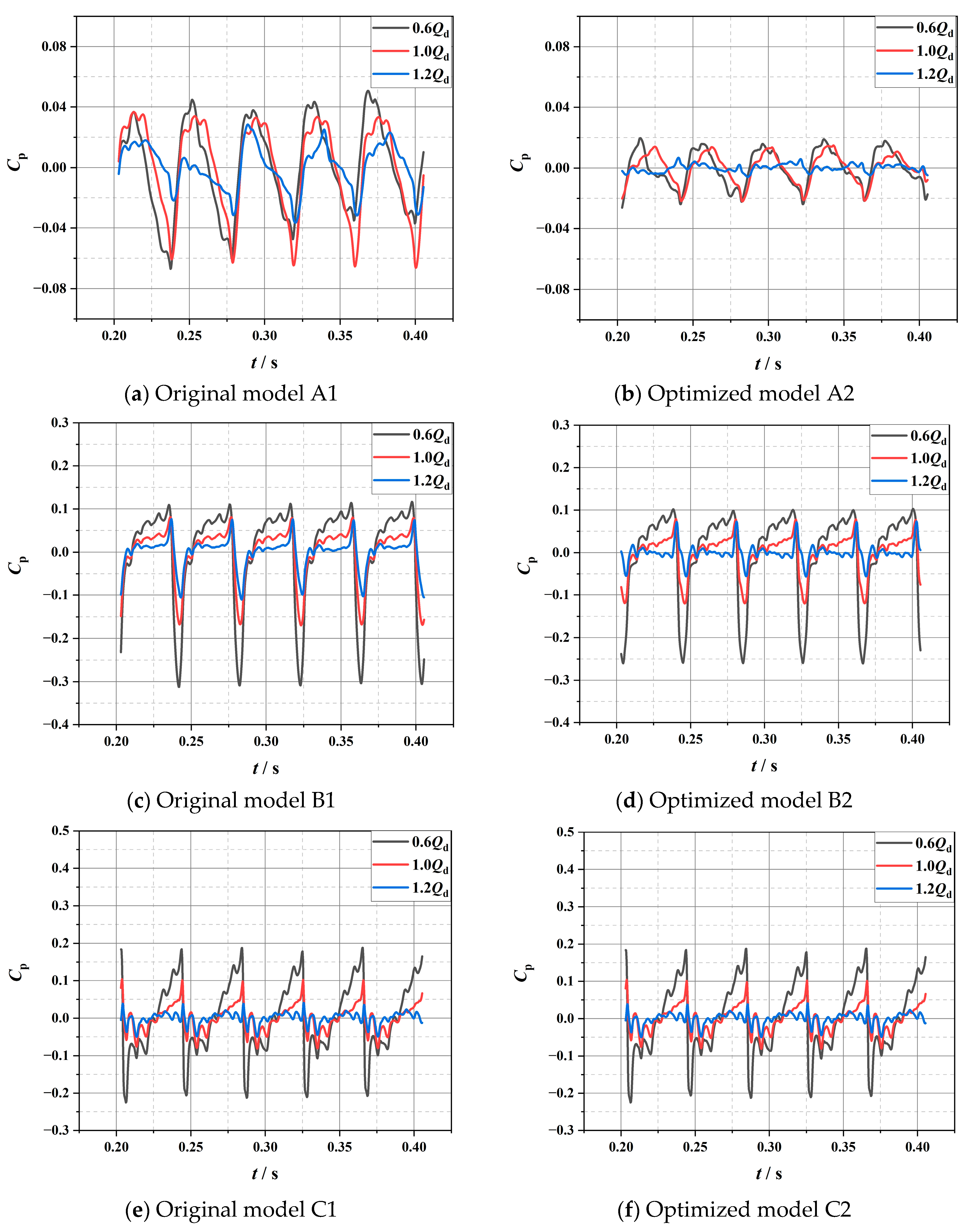
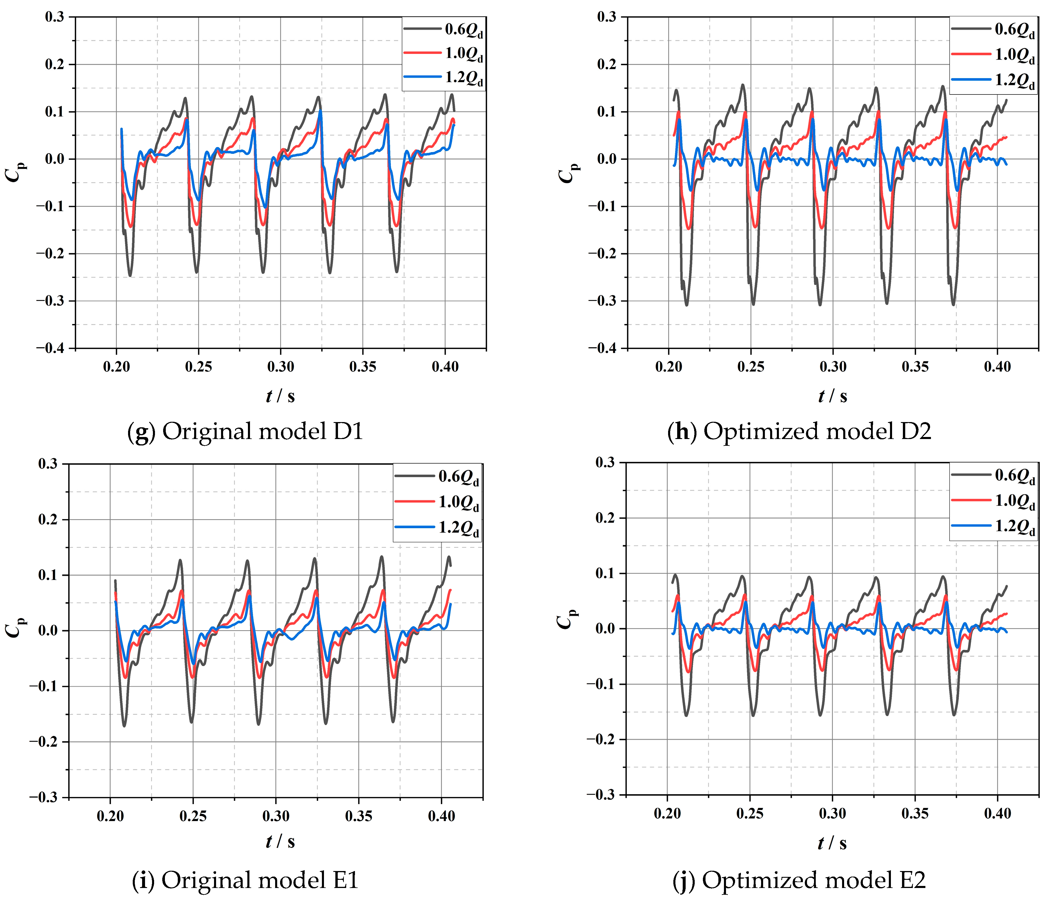
4.3. Analysis of Pressure Fluctuation

4.3.1. Analysis of Impeller Pressure Fluctuation

The change in pressure with time is obtained by calculating the unsteady calculation. Simultaneously, the dimensionless coefficient C_p of pressure fluctuation is incorporated.

$$C_{\mathrm{p}}=\frac{p-\overline{p}}{0.5\rho u_2^2}$$

(21)

where p represents the instantaneous pressure of the monitoring point, for which the unit is Pa; $\overline{p}$ represents the average pressure of the monitoring point within the sampling period, for which the unit is Pa; $\rho$ represents the fluid density, for which the unit is kg/m³; and u₂ represents the impeller outlet peripheral speed, for which the unit is m/s.

To observe the pressure variation trend at each monitoring point, the Fast Fourier Transform (FFT) is employed to convert the time domain result into the frequency domain result. The speed of this pump is 1480 r/min. According to f = nZ/60, the shaft frequency (f_n) is 24.67 Hz, and the blade passing frequency (f_BPF) is 148 Hz. To provide a more intuitive representation of the frequency domain traits of pressure pulsations, the concept of the St (St = f/f_BPF) is introduced, which is the multiple of the blade frequency.

Figure 20 depicts the time domain diagram illustrating pressure fluctuations at distinct monitoring points within the impeller across various flow conditions (Q/Q_d = 0.6, 1.0, and 1.2).

Figure 20 shows the noticeable periodicity of pressure fluctuations at monitoring points on the blade pressure surface and the suction surface under different flow conditions. Notably, all monitoring points exhibit five distinct peaks and troughs. The pressure fluctuation within the pump intensifies progressively from the leading edge to the trailing edge, and the pressure fluctuation at the pressure surface is greater than at the suction surface. Under partial load flow conditions, the pressure fluctuation becomes most pronounced, and its amplitude gradually diminishes with escalating flow rates. This phenomenon can be attributed to the shedding of eddy currents occurring under partial load flow conditions. In comparison to the original model, the optimized model has made improvements in the pressure fluctuations at four monitoring points: A2, B2, C2, and E2. These improvements are particularly noticeable under partial load flow conditions and design conditions. The optimization has improved the unsteady flow within the impeller flow field. Compared with other monitoring points, the pressure fluctuation at monitoring point A1 is more disordered and irregular. Due to the fluid colliding with the blade leading edge when it enters the impeller, backflow and unstable fluctuations are formed. Meanwhile, compared with monitoring point D1 on the trailing edge of the blade, it becomes evident that monitoring point D2 exhibits heightened pressure fluctuations under partial load flow conditions, which may be due to the velocity inconsistency between the impeller and volute of the optimized model, and a small eddy current area is created.

Figure 21 depicts the frequency domain diagram of pressure pulsation under various flow conditions (Q/Q_d = 0.6, 1.0, and 1.2). The diagram reveals that the primary frequency is the shaft frequency (f_n), while the secondary frequencies correspond to its multiples. Furthermore, the amplitude of pressure fluctuations exhibits a gradual rise from the leading edge to the trailing edge of the blade. Significantly, the impeller outlet reaches the highest pressure level. And as the flow rate increases at the same monitoring point, the amplitude of the pressure pulsation decreases. Comparing Figure 19a,b, irregular pulsation is evident at monitoring point A1 of the original model under partial load flow conditions and overload flow conditions, with a relatively high pulsation amplitude. In contrast, the pressure pulsations within the optimized impeller yields a marked reduction in the amplitude of the primary frequency. Simultaneously, under partial load flow conditions, the pressure pulsations and frequency amplitudes at monitoring points B1, E1, B2, and E2 exhibit consistent variation trends. The optimized model effectively diminishes the amplitude of pressure pulsations under both design and overload flow conditions. By comparing the monitoring point C2 on the pressure surface trailing edge of the optimized impeller with the monitoring point C1 of the original impeller, minimal differences are observed in the amplitude of the primary frequency under partial load flow and design conditions. Furthermore, in comparison to the monitoring point D1, the monitoring point D2 exhibits a reduction in the amplitude of the primary frequency under overload flow conditions, a minor difference in amplitude under design condition, and a slight increase in amplitude under partial load flow conditions. This phenomenon arises due to the optimized model’s narrower and elongated flow path. When the flow rate is low, the velocity of the impeller discharge is incongruent with that of the volute, resulting in a slight increase in the amplitude of the pressure pulsation coefficient at this location.

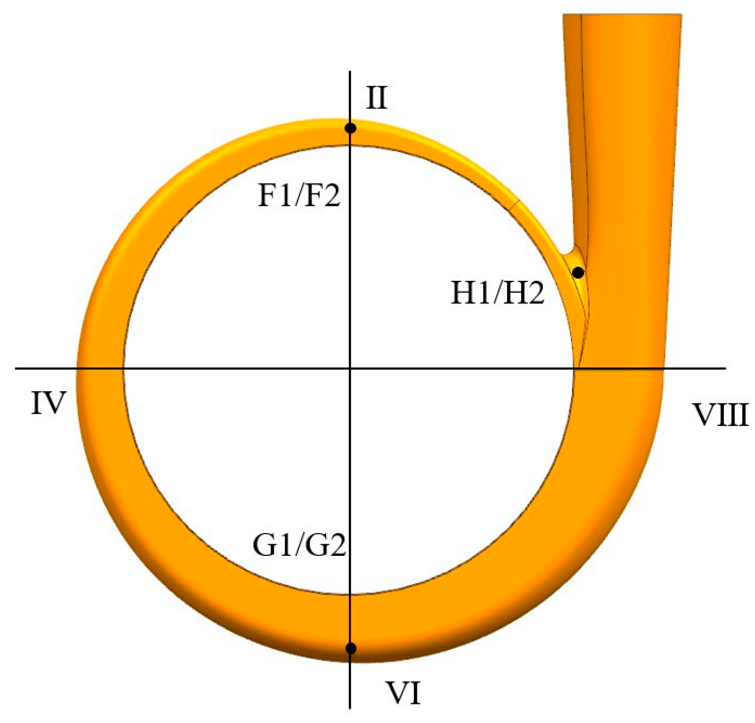
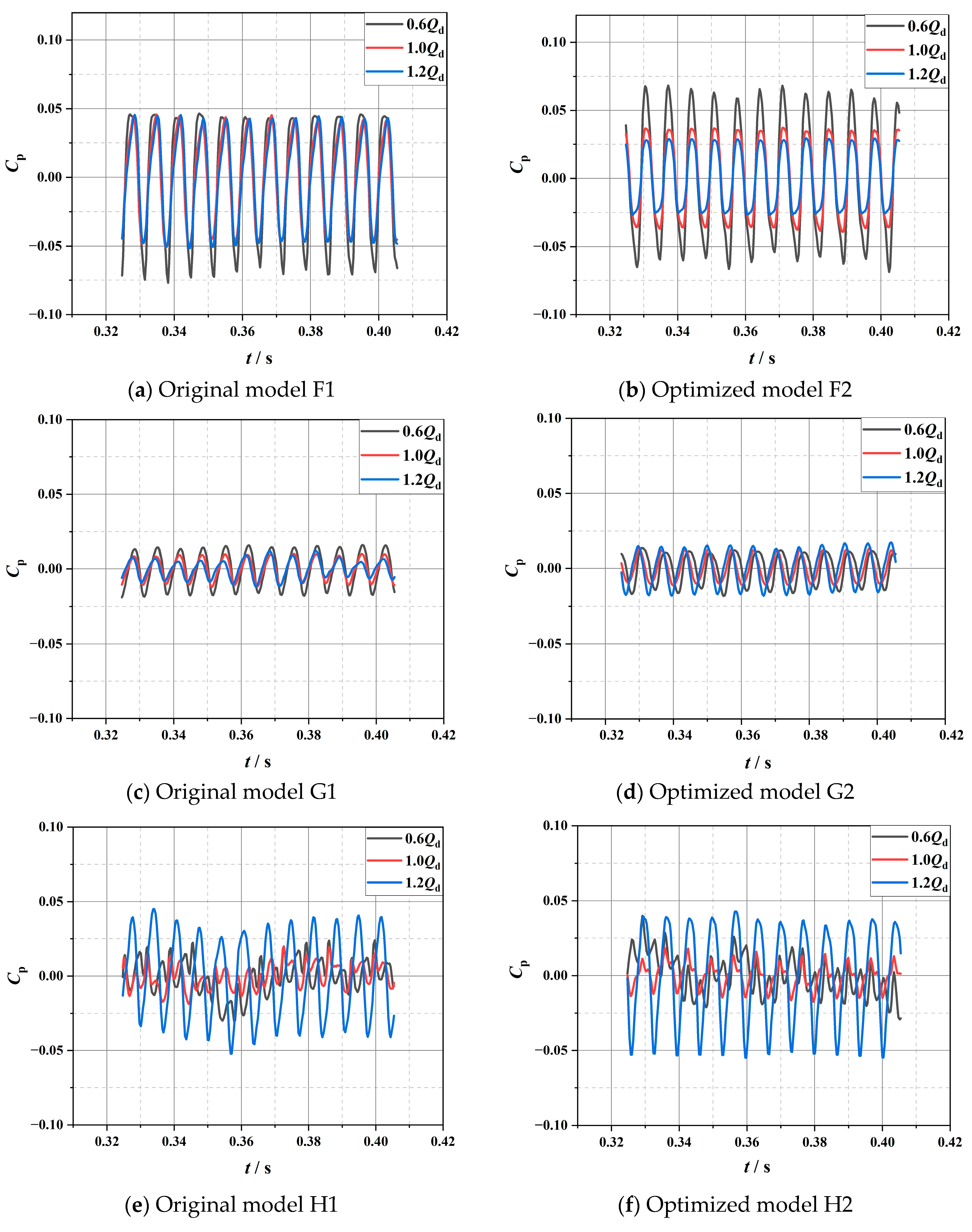
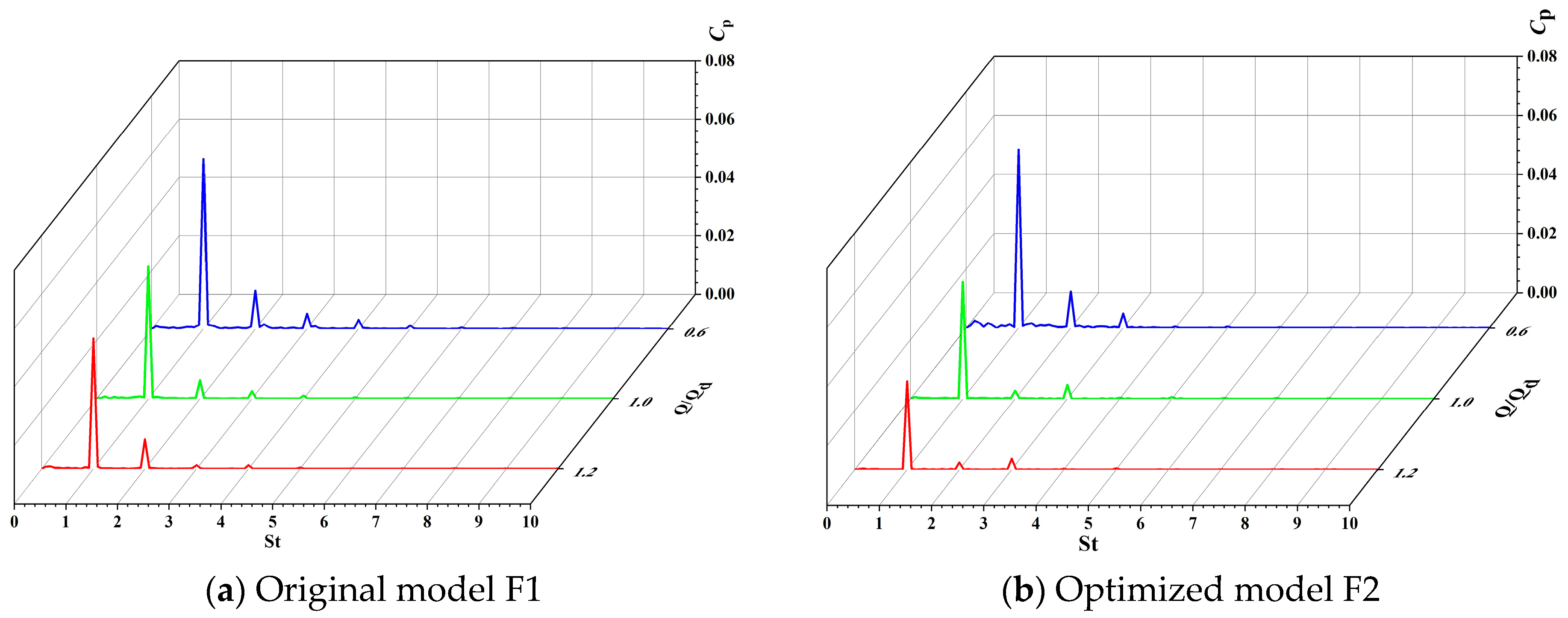
4.3.2. Analysis of Volute Pressure Fluctuation

Figure 22 shows the time domain diagram of the pressure fluctuation under different flow conditions (Q/Q_d = 0.6, 1.0, and 1.2).

In Figure 22, both monitoring points F1 and F2 observed the same phenomenon of six peaks and troughs. This observation indicates that the primary source of pressure pulsation is the dynamic and static interaction between the impeller and the volute. It is worth noting that the optimized model reveals that the issue of pressure pulsation is particularly severe under partial load flow conditions. However, under design conditions and overloaded flow conditions, the condition of pressure pulsation is significantly decreased. The pressure pulsations at monitoring point G1 and G2 in section VI of the volute are significantly smaller than in section II of the volute. This observation highlights the complex flow generated in the vicinity of the tongue area. Additionally, both the amplitude and instability of the pressure pulsations significantly decrease as the monitoring points move away from the tongue area. Furthermore, under partial load flow conditions, the pressure pulsations observed at monitoring points H1 and H2, situated in the vicinity of the tongue area, exhibit periodic weakening compared to the other monitoring points. This phenomenon can be attributed to the formation of backflow vortices near the tongue. However, as the flow rate increases, the periodic nature of these pressure pulsations becomes more pronounced. A significant fluctuation in pressure pulsation is observed in the optimized and original model under overload flow conditions. This phenomenon can be attributed to the intensified impact on the tongue as the fluid velocity in the volute escalates with higher flow rates, ultimately leading to severe pressure pulsations.

Figure 23 shows the frequency domain diagram of the pressure fluctuation under different flow conditions. The primary frequency component for all monitoring points corresponds to the blade passing frequency (f_BPF). Additionally, the secondary frequency components correspond to the harmonics of the blade frequency (f_BPF), further confirming that the pressure pulsations originate from the dynamic and static interference between the impeller and the volute. As the flow rate increases, the amplitude of pressure pulsation at monitoring points F1 and F2 continuously reduces. Furthermore, the amplitude of pressure pulsation at monitoring point F2 is inferior to that at F1, implying that the fluid flow conditions have been effectively improved in the optimized model. Additionally, the amplitude of pressure pulsation at monitoring points G1 and G2 are comparatively lower than those at F1 and F2, which are located farther away from the tongue. The difference between the pulsation amplitude of the optimized and original model is small under the partial load flow conditions and the design conditions, but the pulsation amplitude is increased under the overload flow conditions. It is because the outflow velocity of the impeller does not coincide with the velocity of the volute. The monitoring point H1 and H2 exhibit irregular pressure fluctuations within the frequency range of 0–2 times the blade frequency across various flow conditions. This phenomenon is ascribed to the collision of the impeller outflow with the tongue, leading to the creation of a stagnation zone and an increase in the pressure gradient. This also signifies that low-frequency pulsations are intricately linked to an unstable fluid flow, which aligns with the distribution of the flow field characteristics within the volute.

5. Conclusions

(1)

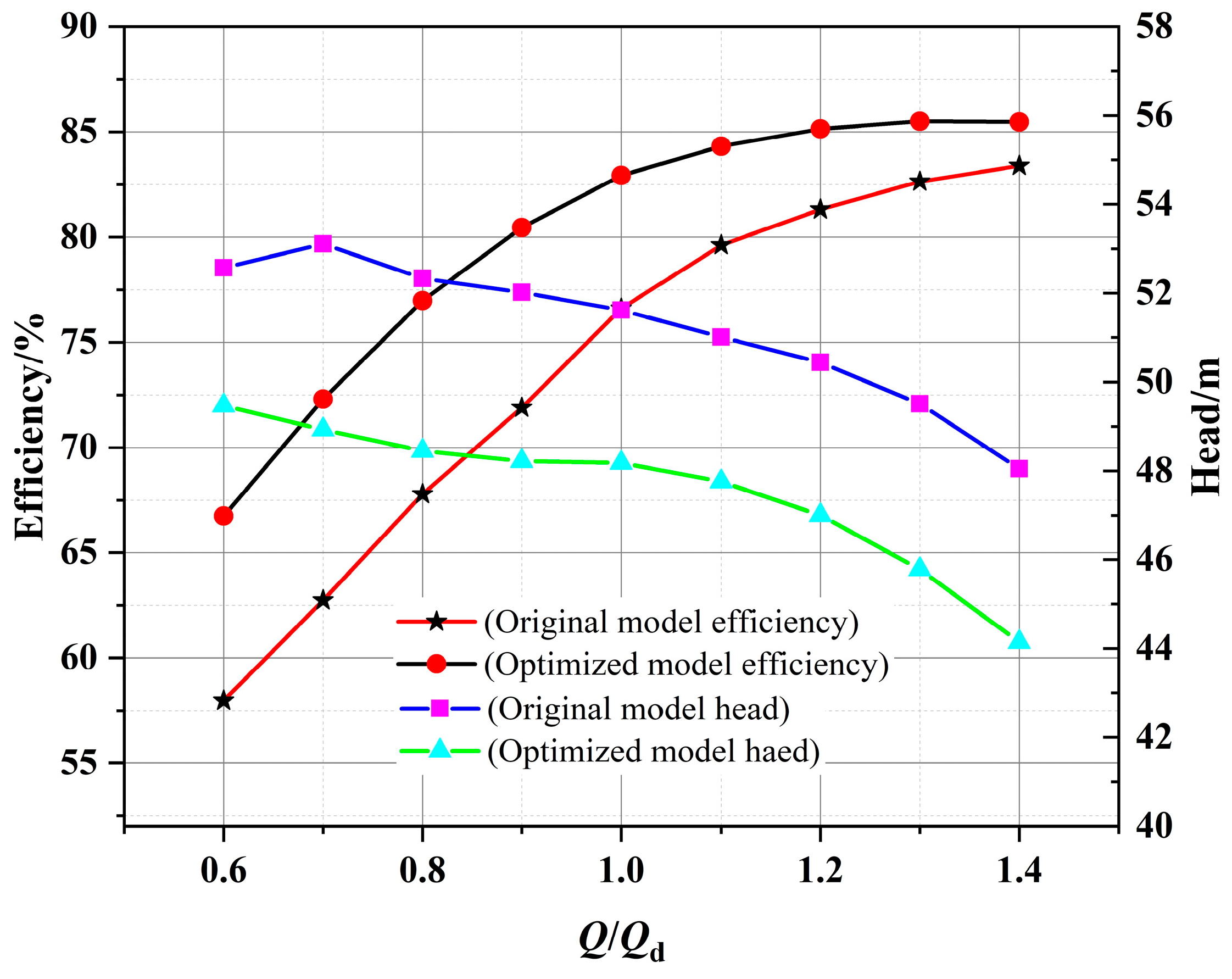
This study takes efficiency as the optimization goal; uses the four key geometric parameters of the impeller blade number Z, blade inlet angle β₁, blade outlet angle β₂, and blade wrap angle φ as optimization variables; and uses the central composite bounded design sampling method to generate the marine sediment pump impeller’s optimization plan. The results of the experimental plan are obtained through parametric modeling and numerical calculations, and the result data are analyzed through response surface optimization. Finally, by solving the regression model, the optimal combination of the optimized impeller model is obtained: Z is 6, β₁ is 32°, β₂ is 17°, and φ is 160°. The optimized model’s efficiency increased by 6.33% under design flow conditions, by more than 2% under overload flow conditions, and by more than 8% under partial load flow conditions. Moreover, the efficient operating area of the marine sediment pump has been significantly expanded. These improvements to the marine sediment pump demonstrate the effectiveness of optimization based on response surface methodology.

(2)

By comparing the flow characteristics and vortex distribution of the original and optimized marine sediment pumps under different flow conditions, this study summarizes the following conclusions. First, in the optimized model, the TKE distribution is more uniform under the design and overload flow conditions, while under partial load flow conditions, there are fewer eddies. Secondly, by using the Omega vortex identification method, it is found that the vortex performance of the original and optimized models had similar changing trends under various flow conditions. Under partial load flow conditions, the flow field vortices of the original model are the most turbulent, while the number of vortex structures of the optimized model is greatly reduced. Finally, compared with the original model, the high-Omega-value areas in the volute section of the optimized model are less distributed and more concentrated, and the streamline distribution is more regular, mainly concentrated on both sides of the volute section, which indicates that the fluid flow characteristics at the outlet of the marine sediment pump have been improved.

(3)

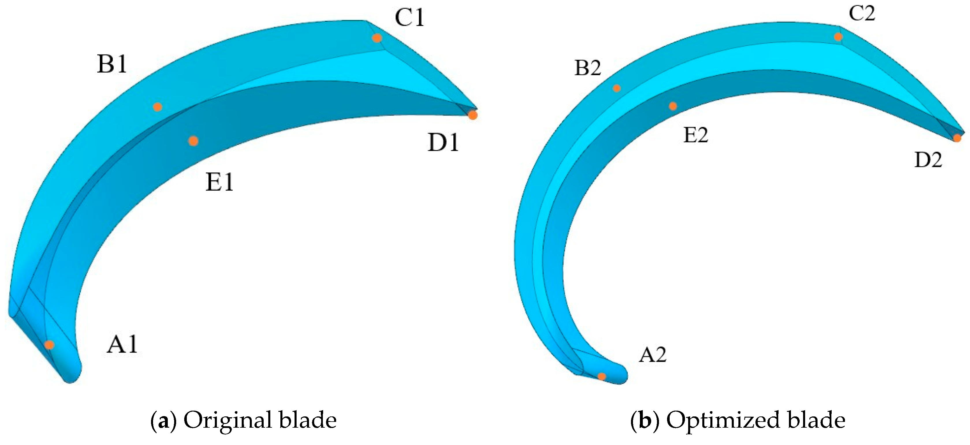
By studying the changing trends of three types of entropy production in marine sediment pumps, it is found that wall entropy production and direct entropy production show a trend of first increasing and then decreasing when the flow rate increased, while turbulent entropy production continued to decrease. Under different flow conditions, the optimized model reduced wall entropy production and turbulence entropy production compared with the original model, while the direct entropy production was reduced by no more than 1%. Exploring the distribution characteristics of total entropy production under different flow conditions shows that the total entropy produced at the volute is the highest, followed by the impeller, then the outlet, and the total entropy production at the inlet is the lowest. Inside the impeller, under partial load flow conditions, the entropy production of the optimized model is lower than that of the original model. However, the entropy production of the optimized model impeller exceeded that of the original model under overload flow conditions and design conditions. This phenomenon is mainly attributed to the increase in impeller wrap angle and blade curvature in the optimization model, which results in an increase in wall entropy production.

(4)

Under different flow conditions, the pressure pulsations of the impeller and volute monitoring points of the original and optimized marine sediment pump are periodic. The main frequency in the impeller frequency domain is the shaft frequency f_n, and the secondary frequency is a multiple of the shaft frequency f_n. The main frequency of the volute monitoring point is the blade passing frequency (f_BPF), and the secondary frequency is the multiple of the blade passing frequency (f_BPF). The pressure pulsation on the impeller gradually increases from the blade leading edge to the blade trailing edge, and the pressure pulsation amplitude on the blade pressure surface is greater than the blade suction surface. Compared with the original impeller, the pressure fluctuations at most monitoring points on the optimized impeller are improved, and the flow is more stable. Under partial load flow conditions, the optimized volute pressure pulsation is particularly serious. However, under the design conditions and overload flow conditions, the pressure pulsation is significantly reduced. Overall, the optimized marine sediment pump model performs better in pressure pulsation compared to the original marine sediment pump model, especially under design and overload flow conditions, showing a more obvious improvement.

References

1. Azizi, R.; Attaran, B.; Hajnayeb, A. Improving accuracy of cavitation severity detection in centrifugal pumps using a hybrid feature selection technique. Meas. J. Int. Meas. Confed. 2017, 108, 9–17. [Google Scholar] [CrossRef]
2. Wu, H. Performance optimization design of sewage pump based on orthogonal experiment. Water Pump Technol. 2021, 6, 13–16. [Google Scholar]
3. Zhang, N.; Li, Z.; Gao, B. Influence of the blade trailing edge profile on the performance and unsteady pressure pulsations in a low specific speed centrifugal pump. J. Fluids Eng. Trans. Asme 2016, 135, 051106. [Google Scholar]
4. Ni, D.; Yang, M.; Gao, B. The internal correlations between unsteady flow and pressure pulsations in a nuclear reactor coolant pump. J. Eng. Thermophys. 2017, 38, 1676–1682. [Google Scholar]
5. Yang, F.; Li, Z.; Fu, J. Numerical and experimental analysis of transient flow field and pressure pulsations of an axial-flow pump considering the pump–pipeline interaction. J. Mar. Sci. Eng. 2022, 10, 258. [Google Scholar] [CrossRef]
6. Zhai, L.; Lu, C.; Guo, J. Flow characteristics and energy loss of a multistage centrifugal pump with blade-type guide vanes. J. Mar. Sci. Eng. 2022, 10, 180. [Google Scholar] [CrossRef]
7. Li, Z.; Zheng, X. Review of design optimization methods for turbomachinery aerodynamics. Prog. Aerosp. Sci. 2017, 93, 1–23. [Google Scholar] [CrossRef]
8. Ren, L. Experimental Design and Optimization; Science Press: Beijing, China, 2009. [Google Scholar]
9. Bashiri, M.; Derakhshan, S.; Shahrabi, J. Design optimization of a centrifugal pump using particle swarm optimization algorithm. Int. J. Fluid Mach. Syst. 2019, 12, 322–331. [Google Scholar] [CrossRef]
10. Wang, W.; Osman, M.; Pei, J. Artificial neural networks approach for a multi-objective cavitation optimization design in a double-suction centrifugal pump. Processes 2019, 7, 23. [Google Scholar] [CrossRef]
11. Xu, M.; Zeng, G.; Wu, D. Structural optimization of jet fish pump design based on a multi-objective genetic algorithm. Energies 2022, 15, 16. [Google Scholar] [CrossRef]
12. Yang, Y.; Zhang, C.; Liu, G. Optimization design of labyrinth seal for piston pump based on response surface method. Fluid Mach. 2021, 49, 44. [Google Scholar]
13. Liu, M.; Tan, L.; Xu, Y. Optimization design method of multi-stage multiphase pump based on Oseen vortex. J. Pet. Sci. Eng. 2019, 184, 106532. [Google Scholar] [CrossRef]
14. Gan, X.; Pei, J.; Wang, W. Application of a modified MOPSO algorithm and multi-layer artificial neural network in centrifugal pump optimization. Eng. Optim. 2022, 55, 580–598. [Google Scholar] [CrossRef]
15. Kim, S.; Yong, K.; Hyung, J. High performance hydraulic design techniques of mixed-flow pump impeller and diffuser. J. Mech. Sci. Technol. 2015, 29, 227–240. [Google Scholar] [CrossRef]
16. Kim, J.; Lee, H. Improvement of hydrodynamic performance of a multiphase pump using design of experiment techniques. J. Fluids Eng. 2015, 137, 081301. [Google Scholar] [CrossRef]
17. Zhang, Y.; Wu, J.; Zhang, Y. Design optimization of centrifugal pump using radial basis function metamodels. Adv. Mech. Eng. 2014, 6, 457542. [Google Scholar] [CrossRef]
18. Yuan, S.; Wang, W.; Pei, J. Multi-objective optimization of low-specific-speed centrifugal pump. J. Agric. Eng. 2015, 31, 46–52. [Google Scholar]
19. Nourbakhsh, A.; Safikhani, H.; Derakhshan, S. The comparison of multi-objective particle swarm optimization and NSGA II algorithm: Applications in centrifugal pumps. Eng. Optim. 2011, 43, 1095–1113. [Google Scholar] [CrossRef]
20. Takayama, Y.; Watanabe, H. Multi-objective design optimization of a mixed-flow pump. Fluids Eng. Div. Summer Meet. 2009, 43727, 371–379. [Google Scholar]
21. Aksoy, M.; Babayigit, O.; Kocaaslan, O. Effect of blade wrap angle to centrifugal pump impeller efficiency. In Proceedings of the International Conference: EFM, Kutná Hora, Czech Republic, 19–22 November 2013; pp. 799–806. [Google Scholar]
22. Shen, J.; Chen, S.; Xu, J. The influence of y+ and turbulence model on the calculation accuracy of the external characteristics of the pump device. China Rural. Water Conserv. Hydropower 2020, 455, 25–29+34. [Google Scholar]
23. Babayigit, O.; Ozgoren, M.; Aksoy, M. Experimental and CFD investigation of a multistage centrifugal pump including leakages and balance holes. Desalin. Water Treat 2017, 67, 28–40. [Google Scholar] [CrossRef]
24. Zhang, N.; Yang, M.; Gao, B. Investigation of rotor-stator interaction and flow unsteadiness in a low specific speed centrifugal pump. Stroj. Vestn. J. Mech. Eng. 2016, 62, 21–31. [Google Scholar] [CrossRef]
25. Gao, B.; Guo, P.; Zhang, N. Unsteady pressure pulsation measurements and analysis of a low specific speed centrifugal pump. J. Fluids Eng. 2017, 139, 071101. [Google Scholar] [CrossRef]
26. Zhang, Y.; Wu, Y. A review of rotating stall in reversible pump turbine. Mech. Eng. Sci. 2017, 231, 1181–1204. [Google Scholar] [CrossRef]
27. Zhang, Y.; Qiu, X.; Chen, F. A selected review of vortex identification methods with applications. J. Hydrodyn. 2018, 30, 767–779. [Google Scholar] [CrossRef]
28. Liu, C.; Wang, Y.; Yang, Y. New omega vortex identification method. Sci. China Phys. Mech. Astron. 2016, 59, 684711. [Google Scholar] [CrossRef]
29. Liu, C.; Gao, Y.; Dong, X. Third generation of vortex identification methods: Omega and Liutex/Rortex based systems. J. Hydrodyn. 2019, 31, 205–223. [Google Scholar] [CrossRef]
30. Zhang, Y.; Liu, K.; Li, J. Analysis of the vortices in the inner flow of reversible pump turbine with the new omega vortex identification method. J. Hydrodyn. 2018, 30, 463–469. [Google Scholar] [CrossRef]
31. Zhao, B.; Liu, Y.; Han, L. Vortex identification and evolution law of mixed flow pump under small flow conditions. Chin. J. Drain. Irrig. Mech. Eng. 2023, 41, 231–238. [Google Scholar]
32. Chang, H.; Shi, W.; Li, W. Energy loss analysis of novel self-priming pump based on the entropy production theory. J. Therm. Sci. 2019, 28, 306–318. [Google Scholar] [CrossRef]
33. Zhou, L.; Hang, J.; Bai, L. Application of entropy production theory for energy losses and other investigation in pumps and turbines: A review. Appl. Energy 2022, 318, 119211. [Google Scholar] [CrossRef]
34. Kock, F.; Herwig, H. Local entropy production in turbulent shear flows: A high-Reynolds number model with wall functions. Int. J. Heat Mass Transf. 2004, 47, 2205–2215. [Google Scholar] [CrossRef]
35. Mathieu, J.; Scott, J. An Introduction to Turbulent Flow; Cambridge University Press: Cambridge, UK, 2000. [Google Scholar]
Figure 1. Marine sediment pump fluid domain model.
Jmse 11 02233 g001
Figure 2. Calculation domain mesh cells.
Jmse 11 02233 g002
Figure 3. Mesh independence verification diagram.
Jmse 11 02233 g003
Figure 4. Comparison of external characteristics between test and simulation.
Jmse 11 02233 g004
Figure 5. Test bench.
Jmse 11 02233 g005
Figure 6. Main effect graphs of single factors on efficiency.
Jmse 11 02233 g006
Figure 7. Two-factor interaction diagram of Z and β2.
Jmse 11 02233 g007
Figure 8. Two-factor interaction diagram of Z and φ.
Jmse 11 02233 g008
Figure 9. Two-factor interaction diagram of β2 and φ.
Jmse 11 02233 g009
Figure 10. Distribution of predictive and actual values of efficiency.
Jmse 11 02233 g010
Figure 11. The blade structure.
Jmse 11 02233 g011
Figure 12. Comparison of external characteristics.
Jmse 11 02233 g012
Figure 13. The location of monitoring points on the impeller blade.
Jmse 11 02233 g013
Figure 14. The arrangement of monitoring points on the volute.
Jmse 11 02233 g014
Figure 15. Turbulent kinetic energy and vortex distribution of the impeller across various flow conditions.
Jmse 11 02233 g015aJmse 11 02233 g015b
Figure 16. Vortex distribution in pump under different flow conditions.
Jmse 11 02233 g016aJmse 11 02233 g016b
Figure 17. Vortex distribution of volute section under different flow conditions.
Jmse 11 02233 g017aJmse 11 02233 g017b
Figure 18. Distribution characteristics of entropy production ratio. (a) Three types of entropy production distributions under different flow conditions. (b) Three types of entropy production ratio distribution under different flow conditions.
Jmse 11 02233 g018
Figure 19. Distribution characteristics of different flow components of entropy production and entropy production ratio. (a) Distribution of entropy production under different flow conditions. (b) Distribution of entropy production ratio under different flow conditions.
Jmse 11 02233 g019
Figure 20. Time domain diagram of impeller monitoring points under different flow conditions.
Jmse 11 02233 g020aJmse 11 02233 g020b
Figure 21. Frequency domain diagram of impeller monitoring points under various flow conditions.
Jmse 11 02233 g021aJmse 11 02233 g021b
Figure 22. Time domain diagram of volute monitoring points under different flow conditions.
Jmse 11 02233 g022
Figure 23. Frequency domain diagram of volute monitoring points under different flow conditions.
Jmse 11 02233 g023aJmse 11 02233 g023b