Enhancing Underwater Robot Manipulators with a Hybrid Sliding Mode Controller and Neural-Fuzzy Algorithm

Abstract

The sliding mode controller stands out for its exceptional stability, even when the system experiences noise or undergoes time-varying parameter changes. However, designing a sliding mode controller necessitates precise knowledge of the object’s exact model, which is often unattainable in practical scenarios. Furthermore, if the sliding control law’s amplitude becomes excessive, it can lead to undesirable chattering phenomena near the sliding surface. This article presents a new method that uses a special kind of computer program (Radial Basis Function Neural Network) to quickly calculate complex relationships in a robot’s control system. This calculation is combined with a technique called Sliding Mode Control, and Fuzzy Logic is used to measure the size of the control action, all while making sure the system stays stable using Lyapunov stability theory. We tested this new method on a robot arm that can move in three different ways at the same time, showing that it can handle complex, multiple-input, multiple-output systems. In addition, applying LPV combined with Kalman helps reduce noise and the system operates more stably. The manipulator’s response under this controller exhibits controlled overshoot (Rad), with a rise time of approximately 5 ± 3% seconds and a settling error of around 1%. These control results are rigorously validated through simulations conducted using MATLAB/Simulink software version 2022b. This research contributes to the advancement of control strategies for robotic manipulators, offering improved stability and adaptability in scenarios where precise system modeling is challenging.

1. Introduction

This scientific analysis focuses on addressing the challenges of precisely controlling underwater robotic arms amidst environmental fluctuations and limitations of traditional control algorithms. This study emphasizes the significance of unmanned underwater machines. These scholarly documents collectively explore remotely operated vehicles (ROVs) for inspection purposes, encompassing a comprehensive review of inspection-class ROVs, the development of an intelligent support system for ROV operators to enhance real-world performance, and the introduction of a novel control method utilizing terminal sliding mode and dynamic damping to improve fault tolerance and predictive capabilities for tracked ROVs [1,2,3], highlighting the roles of robotic arms. These studies also investigate the impact of machining trajectory on grinding force for complex-shaped stone by a robotic manipulator, apply adaptive neural-PID visual servoing tracking control using an Extreme Learning Machine (ELM), and model impedance control with limited interaction power for a 2R planar robot arm [4,5,6] or manipulators [7,8] in conducting complex underwater tasks beyond human reach. These manipulators, operated via controllers like joysticks, are designed for diverse missions, varying in size and strength, and are equipped with hydraulic or electric power, along with sensory or visual aids.

This paper presents a solution that integrates Sliding Mode Control (SMC) [9,10,11,12,13,14] and Radial Basis Function Neural Networks (RBFNN) to enhance the stability and accuracy of a three-degree-of-freedom robotic arm in underwater environments. SMC, known for its stability amidst noise and variable parameters, requires accurate model knowledge, which is complemented by RBFNN’s ability to estimate nonlinear functions online. Additionally, fuzzy logic is proposed to mitigate oscillations around the sliding surface [15,16].

This research incorporates dynamic equations development for the ROV manipulator arm, designing sliding mode, fuzzy logic, and neural-network control systems, and includes noise calculations. It compares the efficacy of these proposed methods with traditional PID control through simulations. Results demonstrate superior performance of the SMC system in amplitude and settling time, with fuzzy logic control achieving the best tracking accuracy, and the neural-network control showing equivalent performance. This research demonstrates the application of neural network-based terminal sliding mode control to space robots actuated by control moment gyros, a novel approach to coordinating large-scale systems with a focus on interaction prediction principles, the utilization of a fuzzy sliding mode controller based on RBF neural network for the control of a three-link robot, the design of adaptive fuzzy sliding-mode control for high-performance islanded inverters in micro-grids, and a comprehensive examination of variable structure control applied to complex systems [17,18,19,20,21].

This paper also acknowledges the use of PID controllers for their simplicity and effectiveness, while highlighting the exploration of neural network and machine-learning approaches for more sophisticated nonlinear control strategies. This study contributes to the field by detailed modeling of robot dynamics, simplifying system-based controller development, and validating the controller on a real robot for balance and path following. This research enhances the understanding and capabilities in designing controllers for self-balancing robots, pushing the boundaries of traditional control methods.

This study addresses the challenges in controlling underwater robotic arms, stemming from the dynamic aquatic environment and the limitations of traditional control methods. It introduces a novel solution combining Sliding Mode Control (SMC) and Fuzzy Neural Network (FNN) to enhance flexibility, precision, and adaptability of the control system [22,23,24]. SMC effectively manages rapid environmental changes, while FNN optimizes the system based on real-time conditions, leading to a more accurate and stable robotic arm control [25] in unpredictable underwater settings.

Experiments conducted under simulated underwater conditions demonstrate that this integrated system significantly outperforms traditional control methods in accuracy and stability. Additionally, this study incorporates the Linear Parameter-Varying (LPV) and Kalman Filter into the system, further improving adaptability and precision. The inclusion of LPV and Kalman Filter makes the control system more versatile, capable of handling underwater variability, and elevates its reliability for high-precision tasks. This advanced approach not only enhances existing systems but also paves the way for developing more accurate and reliable underwater robotic technologies.

This research paper begins with an introduction highlighting the challenges in precisely controlling underwater robotic arms due to environmental fluctuations and limitations of traditional control algorithms. It emphasizes the importance of remotely operated vehicles (ROVs) and robotic manipulators for complex underwater tasks. The second section describes the dynamic modeling of a three-degree-of-freedom robotic arm, outlining its kinetic equations and Denavit–Hartenberg parameters. Next, the adaptive sliding control method is presented, integrating the Sliding Mode Control (SMC) and Radial Basis Function Neural Networks (RBFNN) to enhance system stability and accuracy. Fuzzy logic control is incorporated to mitigate oscillations. Meanwhile, the RBFNN estimates nonlinear functions within the control laws. The Results and Discussion section analyzes the simulation outcomes, comparing the efficacy of the proposed approach to conventional PID controllers in parameters such as rise time, settling error and noise elimination. Finally, the conclusion summarizes the vital contributions of this research in advancing underwater robotic control strategies amidst environmental unpredictability and model limitations. Overall, this study aims to develop an adaptive, stable and high-precision control solution for underwater manipulators.

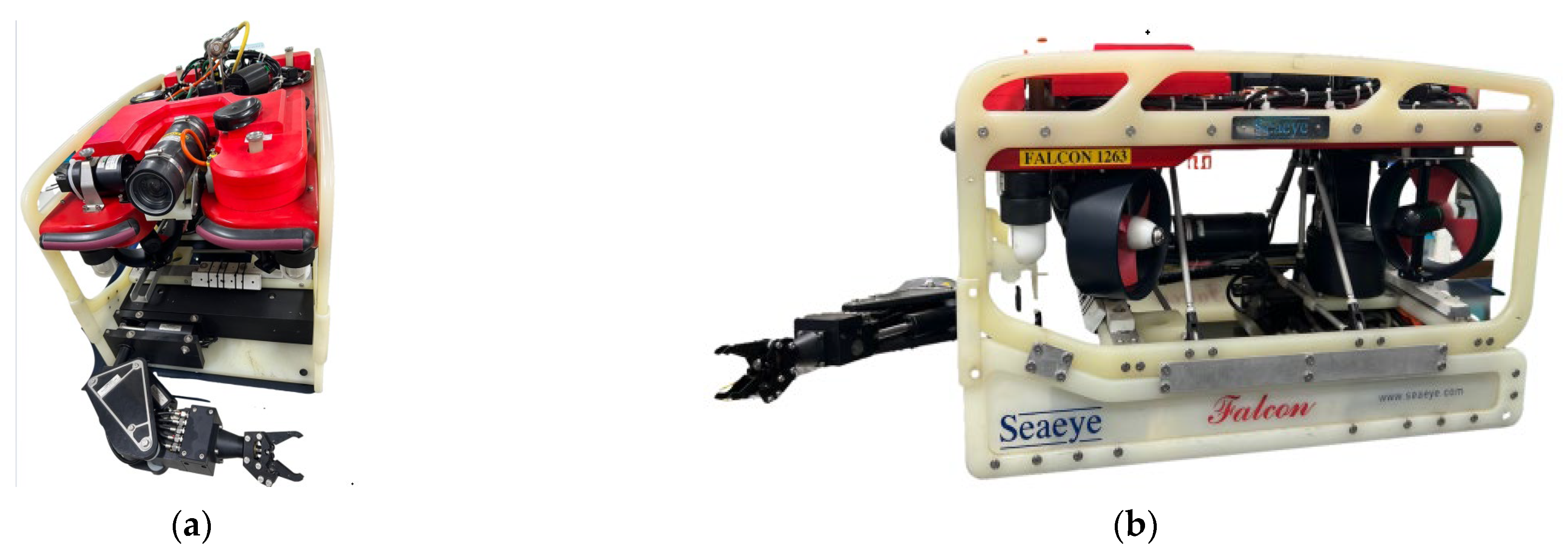
2. Robot Manipulator of Fancon 1263 Model

2.1. A Brief Overview of the Robotic Arm in This Research Paper

The ROV, or Remotely Operated Vehicle, is a purpose-built underwater apparatus equipped with propellers, cameras, and a manipulator arm. The ROV’s body is constructed from a specialized aluminum alloy designed to be both lightweight and durable for marine environments. Its propellers provide omnidirectional mobility, enabling the ROV to move freely in all directions. The manipulator arms of the ROV are highly articulated, often exceeding 1 m in length, and can be fitted with various specialized tools such as welding, cutting, gripping, and holding devices, depending on the specific task requirements.

The simplistic structure of the ROV’s robotic arm is illustrated in Figure 1, which serves as the model referred to, and extensively studied by, the author throughout this research paper.

This study analyzes a Remotely Operated Vehicle (ROV), an unmanned underwater vehicle, detailing its structure as shown in Figure 1. The ROV features a sturdy, watertight body, essential for underwater operation, housing internal electronics, and powered by thrusters for various underwater movements. It is also equipped with cameras and sensors for capturing and relaying underwater images and data.

A crucial element of the ROV is its manipulator arm, designed for precision tasks like grasping and welding, with a simple structure and three degrees of freedom, each link being about 1 m long. This arm, capable of rotational movements, is crucial for underwater maintenance and is remotely operated. It faces challenges like friction and communication delays, which this study addresses with advanced control methods. The arm’s design, affixed to the mobile ROV, allows for a 3 m operational range.

This paper also examines the arm’s dynamic model, a system of differential equations incorporating factors like gravity, buoyancy, and hydrodynamics, using the Lagrange–Euler formulation for modeling. The arm’s kinematics are described using Denavit–Hartenberg parameters, linking joint torques to movements.

This dynamic model is vital for the control system’s development, forming the mathematical basis for controller design, and ensuring optimal performance by accurately modeling system dynamics.

Given the relatively uncomplicated nature of ROV tasks, the authors of this study have utilized a three-degrees-of-freedom manipulator as the subject of investigation. The kinetic model for this three-degree-of-freedom manipulator system is outlined in reference [18]:

$$\mathrm{M}\left(\mathsf{\theta }\right)\ddot{\mathsf{\theta }}+\mathrm{C}\left(\mathsf{\theta },\stackrel{.}{\mathsf{\theta }}\right)\stackrel{.}{\mathsf{\theta }}+\mathrm{F}\left(\mathsf{\theta },\stackrel{.}{\mathsf{\theta }}\right)+\mathrm{G}\left(\mathsf{\theta }\right)+{\mathrm{d}}_{\mathrm{v}}\left(\mathrm{t}\right)=\mathrm{u}$$

(1)

With $\mathrm{M}=\left[\begin{array}{ccc}{\mathrm{M}}_{11}& {\mathrm{M}}_{12}& {\mathrm{M}}_{13}\\ {\mathrm{M}}_{21}& {\mathrm{M}}_{22}& {\mathrm{M}}_{23}\\ {\mathrm{M}}_{31}& {\mathrm{M}}_{32}& {\mathrm{M}}_{33}\end{array}\right]$ is the inertial matrix, $\mathrm{F}={\left[\begin{array}{ccc}{\mathrm{F}}_1& {\mathrm{F}}_2& {\mathrm{F}}_3\end{array}\right]}^{\mathrm{T}}$ is the friction vector, $\mathrm{G}={\left[\begin{array}{ccc}{\mathrm{G}}_1& {\mathrm{G}}_2& {\mathrm{G}}_3\end{array}\right]}^{\mathrm{T}}$ is the gravity vector, ${\mathrm{d}}_v\left(\mathrm{t}\right)$ is the noise signal, $\mathrm{u}={\left[\begin{array}{ccc}{\mathrm{u}}_1& {\mathrm{u}}_2& {\mathrm{u}}_3\end{array}\right]}^{\mathrm{T}}$ is the control signal vector, $\mathsf{\theta }={\left[\begin{array}{ccc}{\mathsf{\theta }}_1& {\mathsf{\theta }}_2& {\mathsf{\theta }}_3\end{array}\right]}^{\mathrm{T}}$ is the angle of the joints of the manipulator system and $\mathrm{C}={\left[\begin{array}{ccc}{\mathrm{C}}_1& {\mathrm{C}}_2& {\mathrm{C}}_3\end{array}\right]}^{\mathrm{T}}$ is expresses the coriolis and centrifugal torques.

$${\mathrm{M}}_{11}=l_1^2\left(\frac{m_1}{3}+m_2+m_3\right)+l_1{l}_2\left(m_2+2m_3\right)\cos \left({\mathrm{q}}_2\right)+I_2^2\left(\frac{m_2}{3}+m_3\right)$$

(2)

$${\mathrm{M}}_{12}={\mathrm{M}}_{21}=m_2\left(l_2^2+l_1{l}_2\cos \left({\mathsf{\theta }}_2 \right)\right)+m_3\left(l_2^2+l_3^2+l_1{l}_2\cos \left({\mathsf{\theta }}_2 \right)\right)+m_3\left(l_1{l}_3\cos \left({\mathsf{\theta }}_2+{\mathsf{\theta }}_3 \right)+2l_2{l}_3\cos \left({\mathsf{\theta }}_3 \right)\right)$$

(3)

$${\mathrm{M}}_{13}={\mathrm{M}}_{31}=m_3\left(l_3^2+l_1{l}_3\cos \left({\mathsf{\theta }}_2+{\mathsf{\theta }}_3 \right)\right)+m_3{l}_2{l}_3\cos ({\mathsf{\theta }}_3)$$

(4)

$${\mathrm{M}}_{22}=m_2{l}_2^2+m_3\left(l_2^2+l_3^2+2l_2{l}_3\cos ({\mathsf{\theta }}_3,)\right)$$

(5)

$${\mathrm{M}}_{23}={\mathrm{M}}_{32}=m_3\left(l_3^2+l_2{l}_3\cos \left({\mathsf{\theta }}_2+{\mathsf{\theta }}_3 \right)\right)$$

(6)

$${\mathrm{M}}_{33}=m_3{l}_3^2$$

(7)

$${\mathrm{F}}_1=-\left(m_2+m_3\right)l_1{l}_2\left(2{\stackrel{.}{\mathsf{\theta }}}_1{\stackrel{.}{\mathsf{\theta }}}_2+{\stackrel{.}{\mathsf{\theta }}}_2^2\right)\sin \left({\mathsf{\theta }}_2\right)-m_3{l}_1{l}_3\mathrm{qsin}\left({\mathsf{\theta }}_2+{\mathsf{\theta }}_3\right)-m_3{l}_2{l}_3\left(2{\stackrel{.}{\mathsf{\theta }}}_1{\stackrel{.}{\mathsf{\theta }}}_3+2{\stackrel{.}{\mathsf{\theta }}}_2{\stackrel{.}{\mathsf{\theta }}}_3+{\stackrel{.}{\mathsf{\theta }}}_3^2\right)\sin \left({\mathsf{\theta }}_3\right)$$

(8)

$${\mathrm{F}}_2=\left(m_2+m_3\right){\stackrel{.}{\mathsf{\theta }}}_1^2\sin \left({\mathsf{\theta }}_2\right)+m_3{l}_1{l}_3{\stackrel{.}{\mathsf{\theta }}}_1^2\sin \left({\mathsf{\theta }}_2+{\mathsf{\theta }}_3\right)-m_3{l}_2{l}_3\left(2{\stackrel{.}{\mathsf{\theta }}}_1{\stackrel{.}{\mathsf{\theta }}}_3+2{\stackrel{.}{\mathsf{\theta }}}_2{\stackrel{.}{\mathsf{\theta }}}_3+{\stackrel{.}{\mathsf{\theta }}}_3^2\right)\sin \left({\mathsf{\theta }}_3\right)$$

(9)

$${\mathrm{F}}_3=m_3{l}_1{l}_3{\stackrel{.}{\mathsf{\theta }}}_1^2\sin \left({\mathsf{\theta }}_2+{\mathsf{\theta }}_3\right)+m_2{l}_2{l}_3\left({\stackrel{.}{\mathsf{\theta }}}_1+{\stackrel{.}{\mathsf{\theta }}}_2\right)\sin \left({\mathsf{\theta }}_3\right)$$

(10)

$$\mathrm{q}=2{\stackrel{.}{\mathsf{\theta }}}_1{\stackrel{.}{\mathsf{\theta }}}_2+2{\stackrel{.}{\mathsf{\theta }}}_1{\stackrel{.}{\mathsf{\theta }}}_3+2{\stackrel{.}{\mathsf{\theta }}}_2{\stackrel{.}{\mathsf{\theta }}}_3+{\stackrel{.}{\mathsf{\theta }}}_2^2+{\stackrel{.}{\mathsf{\theta }}}_3^2$$

(11)

$${\mathrm{G}}_1=m_{1}g{l}_1\cos \left({\mathsf{\theta }}_1\right)+m_{2}g\left(l_2\cos \left({\mathsf{\theta }}_1+{\mathsf{\theta }}_2\right)+l_1\cos \left({\mathsf{\theta }}_1\right)\right)+m_{3}g\left(l_2\cos \left({\mathsf{\theta }}_1+{\mathsf{\theta }}_2\right)+l_1\cos \left({\mathsf{\theta }}_1\right)\right)+m_{3}g\left(l_3\cos \left({\mathsf{\theta }}_1+{\mathsf{\theta }}_2+{\mathsf{\theta }}_3\right)\right)$$

(12)

$${\mathrm{G}}_2=m_{2}g{l}_2\cos \left({\mathsf{\theta }}_1+{\mathsf{\theta }}_2\right)+m_{3}g\left(l_2\cos \left({\mathsf{\theta }}_1+{\mathsf{\theta }}_2\right)\right)+m_{3}g\left(l_3\cos \left({\mathsf{\theta }}_1+{\mathsf{\theta }}_2+{\mathsf{\theta }}_3\right)\right)$$

(13)

$${\mathrm{G}}_3=m_{3}g\left(l_3\cos \left({\mathsf{\theta }}_1+{\mathsf{\theta }}_2+{\mathsf{\theta }}_3\right)\right)$$

(14)

$$C_1={{\displaystyle \sum }}_{j=1}^3{{\displaystyle \sum }}_{k=1}^3 {\Gamma }_{1jk}\left(\theta \right){\stackrel{·}{\theta }}_j{\stackrel{·}{\theta }}_k$$

(15)

$$C_2={{\displaystyle \sum }}_{j=1}^3{{\displaystyle \sum }}_{k=1}^3 {\Gamma }_{2jk}\left(\theta \right){\stackrel{·}{\theta }}_j{\stackrel{·}{\theta }}_k$$

(16)

$$C_3={{\displaystyle \sum }}_{j=1}^3{{\displaystyle \sum }}_{k=1}^3 {\Gamma }_{3jk}\left(\theta \right){\stackrel{·}{\theta }}_j{\stackrel{·}{\theta }}_k$$

(17)

$${\Gamma }_{ijk}\left(\theta \right)=\frac{1}{2}\left(\frac{\mathsf{\partial }{M}_{ij}}{\mathsf{\partial }{\theta }_k}+\frac{\mathsf{\partial }{M}_{ik}}{\mathsf{\partial }{\theta }_j}-\frac{\mathsf{\partial }{M}_{jk}}{\mathsf{\partial }{\theta }_i}\right)$$

(18)

The parameters of the manipulator considered in this study are:

$m_1$ = 1 kg is the mass of joint 1,

$m_2$ = 0.8 kg is the mass of joint 2,

$m_3$ = 0.5 kg is the mass of joint 3,

$l_1$ = 1 m is the length of joint 1,

$l_2$ = 0.8 m is the length of joint 2,

$l_3$ = 0.6 m is the length of joint 3,

g = 9.81 m/s² is the acceleration due to gravity.

${\Gamma }_{ijk}\left(\theta \right)$ are Christoffel symbols.

$M_{ij}, M_{ik}, M_{jk}$ are the elements of the inertia matrix.

2.2. Forward Kinematics

It has been given that there exists a matrix ${\mathrm{T}}_{\mathrm{i}}^{\mathrm{i}-1}$ that is called a homogeneous transformation matrix, and it has the form:

$${\mathrm{T}}_{\mathrm{i}}^{\mathrm{i}-1}=\left[\begin{array}{cc}{\mathrm{R}}_{\mathrm{i}}& {\mathrm{p}}_{\mathrm{i}}\\ 0& 1\end{array}\right]$$

(19)

where: $R_i$ (3 × 3 matrix): rotation matrix.

$p_i$ (3 × 1 matrix): translation vector.

$${\mathrm{T}}_{\mathrm{n}}^0={\displaystyle \prod }_{\mathrm{i}=1}^{\mathrm{n}}{\mathrm{T}}_{\mathrm{i}}^{\mathrm{i}-1}=\left[\begin{array}{cccc}{\mathrm{n}}_{\mathrm{x}}& {\mathrm{o}}_{\mathrm{x}}& {\mathrm{a}}_{\mathrm{x}}& {\mathrm{p}}_{\mathrm{x}}\\ {\mathrm{n}}_{\mathrm{y}}& {\mathrm{o}}_{\mathrm{y}}& {\mathrm{a}}_{\mathrm{y}}& {\mathrm{p}}_{\mathrm{y}}\\ {\mathrm{n}}_{\mathrm{z}}& {\mathrm{o}}_{\mathrm{z}}& {\mathrm{a}}_{\mathrm{z}}& {\mathrm{p}}_{\mathrm{z}}\\ 0& 0& 0& 1\end{array}\right]$$

(20)

where:

n: the number of robot’s joints.

${\mathrm{T}}_{\mathrm{i}}^{\mathrm{i}-1}$: the transformation matrix from coordinate system i to coordinate system i − 1.

${\mathrm{T}}_{\mathrm{n}}^0=\mathrm{f}\left(q_1, q_2, q_{3,\dots , } q_n\right); q_1÷q_n$ are joint variables; n, s, and a are vectors indicating directions, $\mathrm{p}={\left[{\mathrm{p}}_{\mathrm{x}},{ \mathrm{p}}_{\mathrm{y}},{ \mathrm{p}}_{\mathrm{z}}\right]}^{\mathrm{T}}$ is position vector.

Hence, by having knowledge of the geometric characteristics of the links and the kinematic rules governing the joints, it is possible to fully ascertain the position and orientation of the manipulator links.

The objective of the forward kinematics problem is to determine the position and orientation of the end-effector when the values of the joint variables are known. Typically, these joint values are expressed as a function of time, denoted as ${\mathrm{q}}_{\mathrm{i}}={\mathrm{q}}_{\mathrm{i}}\left(\mathrm{t}\right)$, and our task is to ascertain the position and orientation of the end-effector corresponding to these specific joint values. To address the forward kinematics problem, it is necessary to establish the kinematic equations of the robot, as outlined in Equation (20).

For reference, we established a coordinate system with its origin at ${\mathrm{O}}_0$, denoted as ${\mathrm{x}}_0$, ${\mathrm{y}}_0$, and ${\mathrm{z}}_0$, as depicted in Figure 2. Another coordinate system, ${\mathrm{O}}_1$, ${\mathrm{x}}_1$, ${\mathrm{y}}_1$, and ${\mathrm{z}}_1$, is positioned at joint 2, where the ${\mathrm{z}}_1$-axis aligns with the second joint axis. Subsequently, coordinate system ${\mathrm{O}}_2$, ${\mathrm{x}}_2$, ${\mathrm{y}}_2$, and ${\mathrm{z}}_2$, has its origin at joint 3, with the ${\mathrm{z}}_2$-axis aligned with the third joint axis and the ${\mathrm{x}}_2$-axis aligned with the gripper direction, pointing toward the jaws. Lastly, coordinate system ${\mathrm{O}}_3$, ${\mathrm{x}}_3$, ${\mathrm{y}}_3$, and ${\mathrm{z}}_3$, has its origin situated at the center of the gripper. The Denavit–Hartenberg (DH) parameter for a robot in angular coordinate system in

Table 1. The Denavit–Hartenberg (DH) parameter table for a robot in angular coordinate system.

Joint	${\mathsf{\alpha }}_{\mathbf{i}}$	${\mathbf{a}}_{\mathbf{i}}$	${\mathbf{d}}_{\mathbf{i}}$	${\mathsf{\theta }}_{\mathbf{i}}$
1	$90°$	$a_1$	$d_1$	$q_1$
2	0	$a_2$	0	$q_2$
3	0	$a_3$	0	$q_3$

.

From the DH parameter table, it can be determining the transformation matrices between coordinate systems:

$${\mathrm{T}}_1^0=\left[\begin{array}{cccc}c{q}_1& 0& s{q}_1& a_1·c{q}_1\\ s{q}_1& 0& -c{q}_1& a_1·s{q}_1\\ 0& 1& 0& d_1\\ 0& 0& 0& 1\end{array}\right]$$

(21)

$${\mathrm{T}}_2^1=\left[\begin{array}{cccc}c{q}_2& -s{q}_2& 0& a_2·c{q}_2\\ s{q}_2& c{q}_2& 0& a_2·s{q}_2\\ 0& 0& 1& 0\\ 0& 0& 0& 1\end{array}\right]$$

(22)

$${\mathrm{T}}_3^2=\left[\begin{array}{cccc}c{q}_3& -s{q}_3& 0& a_3·c{q}_3\\ s{q}_3& c{q}_3& 0& a_3·s{q}_3\\ 0& 0& 1& 0\\ 0& 0& 0& 1\end{array}\right]$$

(23)

where, abbreviation symbols are used as follows: ${\mathrm{cq}}_1=\cos \left({\mathrm{q}}_1\right),{ \mathrm{sq}}_1=\sin \left({\mathrm{q}}_1\right)·$

The homogeneous transformation matrix representing the position and orientation of the end effector with respect to the origin coordinate system can be determined.

$${\mathrm{T}}_3^0={\mathrm{T}}_1^0·{\mathrm{T}}_2^1·{\mathrm{T}}_3^2=\left[\begin{array}{cccc}c{q}_1·c\left(q_2+q_3\right)& -c{q}_1·s\left(q_2+q_3\right)& s{q}_1& c{q}_1·\left[a_3·s\left(q_2+q_3\right)+a_2·s{q}_2+a_1\right]\\ s{q}_{1}c\left(q_2+q_3\right)& -s{q}_1·s\left(q_2+q_3\right)& -c{q}_1& s{q}_1·\left[a_3·s\left(q_2+q_3\right)+a_2·s{q}_2+a_1\right]\\ s\left(q_2+q_3\right)& c\left(q_2+q_3\right)& 0& a_3·s\left(q_2+q_3\right)+a_2·s{q}_2+a_1\\ 0& 0& 0& 1\end{array}\right]$$

(24)

The dynamic equations of the robot in the angular coordinate system can be acquired by matching corresponding elements of two matrices (${\mathrm{T}}_{\mathrm{n}}^0$ and ${\mathrm{T}}_3^0$).

$$\left\{\begin{array}{c}{n}_x=cos\left(q_1\right)·cos\left(q_2+q_3\right)\hfill \\ n_y=sin\left(q_1\right)·cos\left(q_2+q_3\right)\hfill \\ n_z=sin\left(q_2+q_3\right)\hfill \\ o_x=-cos\left(q_1\right)·sin\left(q_2+q_3\right)\hfill \\ o_y=-sin\left(q_1\right)·sin\left(q_2+q_3\right)\hfill \\ o_z=cos\left(q_2+q_3\right)\hfill \\ a_x=sin\left(q_1\right)\hfill \\ a_y=-cos\left(q_1\right)\hfill \\ a_z=0\hfill \\ p_x=cos\left(q_1\right)·\left[a_3·cos\left(q_2+q_3\right)+a_2·cos\left(q_2\right)+a_1\right]\hfill \\ p_y=sin\left(q_1\right)·\left[a_3·cos\left(q_2+q_3\right)+a_2·cos\left(q_2\right)+a_1\right]\hfill \\ p_z=a_3·sin\left(q_2+q_3\right)+a_2·sin\left(q_2\right)+d_1\hfill \end{array}\right.$$

(25)

2.3. Inverse Kinematics

The inverse kinematics problem necessitates determining the robot’s joint values based on the known position and orientation of the end effector point. These parameters are deduced from a given motion trajectory of the robot, commonly represented in matrix form.

$${\mathrm{T}}_0^{\mathrm{n}}=\left[\begin{array}{cccc}{n}_x& o_x& a_x& p_x\\ n_y& o_y& a_y& p_y\\ n_z& o_z& a_z& p_z\\ 0& 0& 0& 1\end{array}\right]$$

(26)

The solution to the inverse kinematics problem is of paramount significance in robot control. In practical applications, there exists prior knowledge regarding the desired position and orientation of the target end effector point to be reached. The objective is to compute the required joint values for meeting the motion criteria. Consequently, the resolution of the inverse kinematics problem holds pivotal importance in ensuring efficient control of the robot’s operations.

From Equations (24) and (26), there are:

$$\begin{array}{cc}\hfill {\mathrm{T}}_3^0={\mathrm{T}}_1^0·{\mathrm{T}}_2^1·{\mathrm{T}}_3^2& =\left[\begin{array}{cccc}{n}_x& o_x& a_x& p_x\\ n_y& o_y& a_y& p_y\\ n_z& o_z& a_z& p_z\\ 0& 0& 0& 1\end{array}\right]\hfill \\ \hfill & =\left[\begin{array}{cccc}c{q}_1·c\left(q_2+q_3\right)& -c{q}_1·s\left(q_2+q_3\right)& s{q}_1& c{q}_1·\left[a_3·s\left(q_2+q_3\right)+a_2·s{q}_2+a_1\right]\\ s{q}_{1}c\left(q_2+q_3\right)& -s{q}_1·s\left(q_2+q_3\right)& -c{q}_1& s{q}_1·\left[a_3·s\left(q_2+q_3\right)+a_2·s{q}_2+a_1\right]\\ s\left(q_2+q_3\right)& c\left(q_2+q_3\right)& 0& a_3·s\left(q_2+q_3\right)+a_2·s{q}_2+a_1\\ 0& 0& 0& 1\end{array}\right]\hfill \end{array}$$

(27)

Deduce:

$${\left[{\mathrm{T}}_1^0\right]}^{-1}·{\mathrm{T}}_3^0={\mathrm{T}}_2^1·{\mathrm{T}}_3^2={\mathrm{T}}_3^1$$

(28)

A homogeneous matrix is a matrix of the form:

$$\mathrm{T}=\left(\begin{array}{cccc}{n}_x& o_x& a_x& p_x\\ n_y& o_y& a_y& p_y\\ n_z& o_z& a_z& p_z\\ 0& 0& 0& 1\end{array}\right)$$

(29)

According to [21], the inverse matrix of matrix T denoted as $T^{-1}$ will be:

$${\mathrm{T}}^{-1}=\left(\begin{array}{cccc}{n}_x& n_y& n_z& -p·n\\ o_x& o_y& o_z& -p·o\\ a_x& a_y& a_z& -p·a\\ 0& 0& 0& 1\end{array}\right)$$

(30)

Substituting into the expression:

$${\mathrm{T}}_2^1·{\mathrm{T}}_3^2=\left(\begin{array}{cccc}cos\left(q_2+q_3\right)& -sin\left(q_2+q_3\right)& 0& a_3·cos\left(q_2+q_3\right)+a_2·cos\left(q_2\right)\\ sin\left(q_2+q_3\right)& cos\left(q_2+q_3\right)& 0& a_3·sin\left(q_2+q_3\right)+a_2·sin\left(q_2\right)\\ 0& 0& 1& 0\\ 0& 0& 0& 1\end{array}\right)$$

(31)

Balancing the corresponding element at row 3, column 4 of the two matrices, obtain:

$$sin\left(q_1\right)·p_x-cos\left(q_1\right)·p_y=0$$

(32)

Deduce:

$$q_1=atan2\left(p_y,p_x\right)$$

(33)

Through the position of the Robot’s end-effector point, also determine the values of the joint variables:

$$\left\{\begin{array}{l}{a}_3·cos\left(q_2+q_3\right)+a_2·cos\left(q_2\right)=cos\left(q_1\right)·p_x+sin\left(q_1\right)·p_y-a_1\hfill \\ a_3·sin\left(q_2+q_3\right)+a_2·sin\left(q_2\right)=p_z-d_1\hfill \end{array}\right.$$

(34)

Deduce:

$$\left\{\begin{array}{l}{q}_2=atan2\left(\frac{p_z-d_1}{cos\left(q_1\right)·p_x+sin\left(q_1\right)·p_y-a_1}\right)-atan\left(\frac{a_3·sin\left(q_3\right)}{a_3·cos\left(q_3\right)+a_2}\right)\hfill \\ q_3=\mp acos\frac{{\left[cos\left(q_1\right)·p_x+sin\left(q_1\right)·p_y-a_1\right]}^2+{\left(p_z-d_1\right)}^2-\left(a_3{ }^2+a_2{ }^2\right)}{2·a_2·a_3}\hfill \end{array}\right.$$

(35)

2.4. Noise When Working Underwater

The resistance forces on a subsea manipulator include:

Frictional resistance: this is the resistance caused by the friction between the surface of the manipulator and the water. This force depends on the manipulator’s speed, the surface area in contact, and the viscosity of the water. The formula for calculating frictional resistance:

$${\mathrm{F}}_{\mathrm{frictional}}=k·v$$

(36)

where:

F is the frictional resistance.

k is the coefficient of friction.

v is the speed of the manipulator.

Pressure resistance: This is the resistance caused by the water pressure acting on the surface of the manipulator. This force depends on the depth below the sea and the speed of the manipulator. The formula for calculating pressure resistance:

$${\mathrm{F}}_{\mathrm{pressure}}=\frac{1}{2} ·\rho ·\mathrm{A}·v^2$$

(37)

where:

F is the pressure resistance.

ρ is the density of the water.

A is the surface area of the manipulator.

v is the speed of the manipulator.

Molecular resistance: this is the resistance caused by water molecules hindering the movement of the manipulator. This force depends on the viscosity of the water and the speed of the manipulator. The formula for calculating molecular resistance:

$${\mathrm{F}}_{\mathrm{molecular}}=6·\pi ·\eta ·r·v$$

(38)

where:

F is the molecular resistance.

η is the viscosity of the water.

r is the radius of the manipulator.

v is the speed of the manipulator.

Impact force is when the ROV changes motion suddenly.

In the process of researching and developing manipulators attached to ROVs, identifying and analyzing sudden forces arising from changes in the ROV’s motion in the system plays an important role. These forces, including inertial forces, centrifugal forces, and Coriolis forces, have a significant influence on the precision and stability of the manipulator. Static force occurs when the ROV accelerates or decelerates suddenly. It is calculated using formula:

$$F_{inertia}=m·a$$

(39)

where: $m$ is the mass of manipulator.

a is the acceleration of the ROV.

This force causes the position of the manipulator to shift. This change can affect the ability to perform tasks accurately, essential in many underwater activities. When the ROV makes rapid changes of direction, the centrifugal force becomes significant. The formula for this force is:

$$F_{centrifugal}=\frac{m·v^2}{r}$$

(40)

where $v$ is the velocity of the ROV and r is the turning radius.

Centrifugal force can cause rotation of the manipulator, affecting its angular position and ability to maintain correct orientation. In the rotating reference frame of the ROV, the Coriolis force becomes important, especially when the ROV changes its angular velocity. The formula for calculating this force is:

$$F_{coriolis}=2m\left(v_x\times \Omega \right)$$

(41)

where $v_x$ is the velocity of the manipulator handle, and

Ω is the angular velocity of the ROV.

This force causes a deflection in the manipulator’s trajectory, requiring adjustment to achieve the correct position. This analysis provides a detailed view of how sudden forces affect the manipulator in the system, highlighting the complexity of underwater robot operations and the need for advanced control strategies to manage these challenges. An in-depth understanding of these effects is necessary to develop control systems capable of eliminating their effects, ensuring that the manipulator operates accurately and stably in full underwater environments.

The total resistive force on the manipulator is calculated by adding up all the resistive forces, namely:

$${\mathrm{F}}_{\mathrm{total}}={\mathrm{F}}_{\mathrm{frictional}}+{\mathrm{F}}_{\mathrm{pressure}}+{\mathrm{F}}_{\mathrm{molecular}}+F_{inertia}+F_{centrifugal}+F_{coriolis}$$

(42)

3. Adaptive Sliding Control Using Neural Network and Logic Fuzzy Controller

3.1. Sliding Mode Control

Sliding mode control (SMC) represents a control system approach employed for stabilizing dynamic systems, particularly those characterized by uncertain or nonlinear dynamics. The fundamental concept underlying SMC is to compel the system to adhere to a specific trajectory or sliding surface within the state space, irrespective of initial system conditions or external disturbances.

Sliding mode control is introduced as a powerful control method capable of achieving stable control of nonlinear systems even in the presence of model uncertainty and external disturbances. The core idea of sliding mode control is to force the system’s states to “slide” along a switching hyperplane (referred to as the sliding surface) toward an equilibrium point. This is achieved by applying a discontinuous control law to switch control actions based on the sign of the error between the current state and the desired state. The switching ensures that the system’s states converge and remain on the sliding surface, providing robustness against model uncertainties and disturbances. To implement sliding mode control, an appropriate sliding surface is first designed based on the system’s dynamics and relative degree. Then, a switching control law is derived, comprising equivalent control terms to compensate for model uncertainties and switching terms to counteract disturbances and bring states onto the sliding surface. In this research paper, the sliding mode control method is applied to control a three-degree-of-freedom robotic arm for underwater operations. Challenges related to model uncertainty and noise in the underwater environment drive the use of sliding mode control. Let ${\mathsf{\theta }}_{\mathrm{d}}$ denote the desired manipulator response, while θ represents the actual output of the manipulator. The primary control objective entails minimizing the error between θ and ${\mathsf{\theta }}_{\mathrm{d}}$, as defined in Equation (43).

$$\mathrm{e}=\mathsf{\theta }-{\mathsf{\theta }}_{\mathrm{d}}$$

(43)

Sliding surface ${\mathrm{s}}_{\mathrm{I}}$ (with $\mathrm{i}=\overline{1,3}$):

$${\mathrm{s}}_{\mathrm{i}}={\stackrel{·}{\mathrm{e}}}_{\mathrm{i}}+{\mathrm{a}}_{\mathrm{i}}{\mathrm{e}}_{\mathrm{i}}$$

(44)

where:

$${\mathrm{a}}_{\mathrm{i}}>0$$

Choose the control law u such that derivative of the sliding surface:

$$\stackrel{·}{\mathrm{e}}=\left[\begin{array}{c}{\stackrel{·}{\mathrm{s}}}_1\\ {\stackrel{.}{\mathrm{s}}}_2\\ {\stackrel{.}{\mathrm{s}}}_3\end{array}\right]=-\left[\begin{array}{c}{\mathrm{k}}_1·\mathrm{sign}\left({\mathrm{s}}_1\right)\\ {\mathrm{k}}_2·\mathrm{sign}\left({\mathrm{s}}_2\right)\\ {\mathrm{k}}_3·\mathrm{sign}\left({\mathrm{s}}_3\right)\end{array}\right]$$

(45)

The control goal is to design u such that $\stackrel{.}{\mathrm{s}}$ is driven to zero exponentially fast, ensuring the system states converge to the sliding surface.

Sliding control law:

$${\mathrm{u}}_{\mathrm{s}}=\left[\mathrm{F}\left(\mathsf{\theta },\stackrel{·}{\mathsf{\theta }}\right)+\mathrm{G}\left(\mathsf{\theta }\right)\right]+\mathrm{M}\left[\begin{array}{c}{\ddot{\mathsf{\theta }}}_{1\mathrm{d}}-{\mathrm{a}}_1\left({\mathsf{\theta }}_1-{\stackrel{·}{\mathsf{\theta }}}_{1\mathrm{d}}\right)-{\mathrm{k}}_1·\mathrm{sign}\left({\mathrm{s}}_1\right)\\ {\ddot{\mathsf{\theta }}}_{2\mathrm{d}}-{\mathrm{a}}_2\left({\mathsf{\theta }}_2-{\stackrel{·}{\mathsf{\theta }}}_{2\mathrm{d}}\right)-{\mathrm{k}}_2·\mathrm{sign}\left({\mathrm{s}}_2\right)\\ {\ddot{\mathsf{\theta }}}_{3\mathrm{d}}-{\mathrm{a}}_3\left({\mathsf{\theta }}_3-{\stackrel{·}{\mathsf{\theta }}}_{3\mathrm{d}}\right)-{\mathrm{k}}_3·\mathrm{sign}\left({\mathrm{s}}_3\right)\end{array}\right]$$

(46)

3.2. Sliding Mode Control-Fuzzy Logic Control

Fuzzy logic is applied to estimate the amplitude of the sliding mode control law in a dynamic, adaptive manner. This helps reduce chattering in the control output. A fuzzy inference system (FIS) is developed using input of error (s) and change in error. Gaussian membership functions are defined for the fuzzy sets of the input and output variables. IF-THEN rules are constructed to relate the fuzzy sets of error to the fuzzy sets of the control gain (k). The FIS evaluates the rules using fuzzy logic operations (in this paper it is AND) to map crisp error values to crisp control gain values. This adaptive, fuzzy-estimated control gain is then used within the overall sliding mode control law to regulate the system states. The use of fuzzy logic is rationalized as it allows modeling nonlinear dynamics and uncertainties in a simple, intuitive way using linguistic rules. This helps sliding mode control accommodate unknown factors in the underwater manipulator system. By integrating fuzzy logic within sliding mode control, the approach aims to leverage the robustness of SMC while reducing chattering through adaptive gain estimation.

Consider the sliding mode control system-Fuzzy Logic control [26,27,28,29]. The amplitude of the control rule is dynamically estimated through a fuzzy inference system utilizing the rules structured as follows:

IF ${\mathrm{s}}_{\mathrm{I}}$ is ${\mathrm{A}}_{\mathrm{i}}^{\mathrm{m}}$ THEN ${\mathrm{k}}_{\mathrm{I}}$ is ${\mathrm{B}}_{\mathrm{i}}^{\mathrm{m}}$

Within $\mathrm{i}=\overline{1,3}$

Where ${\mathrm{A}}_{\mathrm{i}}^{\mathrm{m}}$ and ${\mathrm{B}}_{\mathrm{i}}^{\mathrm{m}}$ are fuzzy sets (Figure 3).

The membership functions used are Gaussian functions [18].

$${\mathsf{\mu }}_{\mathrm{A}}\left({\mathrm{s}}_{\mathrm{i}}\right)=\exp \left(-{\left(\frac{{\mathrm{s}}_{\mathrm{i}}-{\mathsf{\alpha }}_{\mathrm{i}}}{{\mathsf{\sigma }}_{\mathrm{i}}}\right)}^2\right)$$

(47)

where:

$\mathrm{i}=\overline{1,3}$, ${\mathrm{k}}_{\mathrm{I}}$ ≥ 0

${\mathsf{\alpha }}_{\mathrm{i}}$, ${\mathsf{\sigma }}_{\mathrm{I}}$ are the center and width of the ith Gaussian function, respectively.

Choose a positive definite function.

$$\mathrm{V}=\frac{1}{2}{\displaystyle \sum }_{\mathrm{i}=1}^3{\mathrm{s}}_{\mathrm{i}}^2$$

(48)

From (47) deduce:

$$\stackrel{·}{\mathrm{V}}=-{\displaystyle \sum }_{\mathrm{i}=1}^3{\mathrm{s}}_{\mathrm{i}}·{\mathrm{k}}_{\mathrm{i}}·\mathrm{sign}\left({\mathrm{s}}_{\mathrm{i}}\right)$$

(49)

$$\stackrel{·}{\mathrm{V}}=-{{\displaystyle \sum }}_{\mathrm{i}=1}^3\left|{\mathrm{s}}_{\mathrm{i}}\right|·{\mathrm{k}}_{\mathrm{i}}$$

(50)

Therefore, the fuzzy rule is defined as follows:

IF $\left|{\mathrm{s}}_{\mathrm{I}}\right|$ is NB THEN ${\mathrm{k}}_{\mathrm{I}}$ is NB

IF $\left|{\mathrm{s}}_{\mathrm{I}}\right|$ is NM THEN ${\mathrm{k}}_{\mathrm{I}}$ is NM

IF $\left|{\mathrm{s}}_{\mathrm{I}}\right|$ is NS THEN ${\mathrm{k}}_{\mathrm{I}}$ is NS

IF $\left|{\mathrm{s}}_{\mathrm{I}}\right|$ is Z THEN ${\mathrm{k}}_{\mathrm{I}}$ is Z

IF $\left|{\mathrm{s}}_{\mathrm{I}}\right|$ is PS THEN ${\mathrm{k}}_{\mathrm{I}}$ is PS

IF $\left|{\mathrm{s}}_{\mathrm{I}}\right|$ is PM THEN ${\mathrm{k}}_{\mathrm{I}}$ is PM

IF $\left|{\mathrm{s}}_{\mathrm{I}}\right|$ is PB THEN ${\mathrm{k}}_{\mathrm{I}}$ is PB

Where:

NB: Negative Big

NM: Negative Medium

NS: Negative Small

Z: Zero

PS: Positive Small

PM: Positive Medium

PB: Positive Big

Program for Fuzzy Logic Control in MATLAB version 2022b that is presented in Appendix A section.

3.3. Sliding Control Using RBFNN Network

An RBFNN is used to estimate nonlinear functions within the sliding mode control law, since an exact mathematical model of the underwater manipulator system is difficult to obtain. The RBFNN consists of three parts—an input layer, a hidden layer with radial basis activation functions, and an output layer. It is trained online using a gradient descent-based algorithm to minimize the error between the actual and desired sliding surfaces. The RBFNN learns and adapts the control law based on current state feedback without requiring an exact model of the system dynamics. This helps make the sliding mode control more robust by compensating for model uncertainties and nonlinearities in the real-world underwater system. The RBFNN also allows the control law to be adjusted continuously in real-time as the system operates, improving tracking performance.

In this research, the strategic selection of the Radial Basis Function Neural Network (RBFNN) marks a significant development in the control of underwater robotic arms. RBFNN is highly valued for its efficient handling of unstable and fluctuating data, a critical characteristic in the challenging underwater environment. This choice presents a clear advantage over other neural-network architectures like Convolutional Neural Networks (CNN) and Long Short-Term Memory (LSTM). While CNNs excel in image processing due to their feature detection capabilities, they may not fully capture the continuous variations of the underwater environment. Similarly, while LSTMs are effective in processing sequential data and long-term information, they might struggle with the rapid and abrupt changes typical in underwater settings. In contrast, RBFNN, with its rapid adaptability and effective handling of unstructured data, emerges as the optimal choice in this scenario. This decision not only reflects a deep understanding of the specific challenges in underwater robotic control but also demonstrates flexibility and creativity in applying AI technology to address complex issues.

In summary, RBFNN is an effective choice in solving prediction, classification, and control problems, especially in real-world environments with noise and uncertainty. In this study, we consider the application of the sliding control system using RBF neural network [29,30,31]. The nonlinear system is given as (51).

$$\left\{\begin{array}{c}\stackrel{·}{\mathrm{x}}=f\left(\mathrm{x}\right)+g\left(\mathrm{x}\right)u \\ y=h\left(x\right) \end{array}\right.$$

(51)

where x = [x₁, x₂, …, x_n]^T is the state vector, u is the input signal, y is the output signal, f(x) and g(x) are the nonlinear functions describing the characteristic kinematics of the system.

Suppose (52) does not contain u and (46) contains u.

$$\frac{{\mathrm{d}}^{\mathrm{r}-1}\mathrm{y}}{{\mathrm{dt}}^{\mathrm{r}-1}}={\mathrm{L}}_{\mathrm{f}}^{\left(\mathrm{r}-1\right)}\mathrm{h}\left(\mathrm{x}\right)+{\mathrm{L}}_{\mathrm{f}}^{\left(\mathrm{r}-2\right)}{\mathrm{L}}_{\mathrm{g}}\mathrm{h}\left(\mathrm{x}\right)$$

(52)

$$\frac{{\mathrm{d}}^{\mathrm{r}}\mathrm{y}}{{\mathrm{dt}}^{\mathrm{r}}}={\mathrm{L}}_{\mathrm{f}}^{\left(\mathrm{r}\right)}\mathrm{h}\left(\mathrm{x}\right)+{\mathrm{L}}_{\mathrm{f}}^{\left(\mathrm{r}-1\right)}{\mathrm{L}}_{\mathrm{g}}\mathrm{h}\left(\mathrm{x}\right)\mathrm{u}$$

(53)

where:

${\mathrm{L}}_{\mathrm{f}}\mathrm{h}\left(\mathrm{x}\right)=\frac{\mathsf{\partial }\mathrm{h}\left(\mathrm{x}\right)}{\mathsf{\partial }\mathrm{x}}\mathrm{f}\left(\mathrm{x}\right)$ is the Lie derivative in the f(x) direction.

${\mathrm{L}}_{\mathrm{g}}\mathrm{h}\left(\mathrm{x}\right)=\frac{\mathsf{\partial }\mathrm{h}\left(\mathrm{x}\right)}{\mathsf{\partial }\mathrm{x}}\mathrm{g}\left(\mathrm{x}\right)$ is the Lie derivative in the g(x) direction.

From (53) deduce:

$${\mathrm{y}}^{\left(\mathrm{r}\right)}=\mathrm{a}\left(\mathrm{x}\right)+\mathrm{b}\left(\mathrm{x}\right)\mathrm{u}$$

(54)

where:

$$\mathrm{a}\left(\mathrm{x}\right)={\mathrm{L}}_{\mathrm{f}}^{\left(\mathrm{r}\right)}\mathrm{h}\left(\mathrm{x}\right)$$

(55)

$$\mathrm{b}\left(\mathrm{x}\right)={\mathrm{L}}_{\mathrm{f}}^{\left(\mathrm{r}-1\right)}{\mathrm{L}}_{\mathrm{g}}\mathrm{h}\left(\mathrm{x}\right)$$

(56)

The control law u is determined such that:

$${\mathrm{y}}^{\left(\mathrm{r}\right)}=\mathrm{v}\left(\mathrm{t}\right)$$

(57)

where v(t) is the new control signal.

From (55)–(57) deduce:

$${\mathrm{u}}^{*}\left(\mathrm{x}\right)=\frac{1}{\mathrm{b}\left(\mathrm{x}\right)}\left[-\mathrm{a}\left(\mathrm{x}\right)+\mathrm{v}\left(\mathrm{t}\right)\right]$$

(58)

The control law v(t) is determined based on the pole assignment method with the characteristic equation:

$${\mathrm{e}}^{\left(\mathrm{r}\right)}+{\mathrm{k}}_1{\mathrm{e}}^{\left(\mathrm{r}-1\right)}+\dots +{\mathrm{k}}_{\mathrm{r}-1}{\mathrm{e}}^1=0$$

(59)

where:

${\mathrm{y}}_{\mathrm{m}}\left(\mathrm{t}\right)$ is the desired output value.

$\mathrm{y}\left(\mathrm{t}\right)$: actual output value

k₁, k₂, …, k_r−1: is chosen so that (59) has a negative definite solution.

$$\mathrm{e}\left(\mathrm{t}\right)={\mathrm{y}}_{\mathrm{m}}\left(\mathrm{t}\right)-\mathrm{y}\left(\mathrm{t}\right)$$

(60)

From (57), (59) and (60) deduce:

$${\mathrm{y}}_{\mathrm{m}}^{\left(\mathrm{r}\right)}\left(\mathrm{t}\right)-\mathrm{v}\left(\mathrm{t}\right)+{\mathrm{k}}_1{\mathrm{e}}^{\left(\mathrm{r}-1\right)}+\dots +{\mathrm{k}}_{\left(\mathrm{r}-1\right)}\mathrm{e}=0$$

(61)

Or:

$${\mathrm{y}}_{\mathrm{m}}^{\left(\mathrm{r}\right)}\left(\mathrm{t}\right)+{\mathrm{k}}_1{\mathrm{e}}^{\left(\mathrm{r}-1\right)}+\dots +{\mathrm{k}}_{\left(\mathrm{r}-1\right)}\mathrm{e}=\mathrm{v}\left(\mathrm{t}\right)$$

(62)

Set [28]:

$${\overline{\mathrm{e}}}_{\mathrm{s}}+{\mathsf{\eta }\mathrm{e}}_{\mathrm{s}}\left(\mathrm{t}\right)={\mathrm{k}}_1{\mathrm{e}}^{\left(\mathrm{r}-1\right)}+\dots +{\mathrm{k}}_{\left(\mathrm{r}-1\right)}\mathrm{e}$$

(63)

where:

$${\mathrm{e}}_{\mathrm{s}}\left(\mathrm{t}\right)={\mathrm{k}}_1{\mathrm{e}}^{\left(\mathrm{r}-1\right)}+{\mathrm{k}}_2{\mathrm{e}}^{\left(\mathrm{r}-2\right)}+\dots +{\mathrm{k}}_{\left(\mathrm{r}-1\right)}\mathrm{e}$$

η: is a positive constant.

$${\overline{\mathrm{e}}}_{\mathrm{s}}={\stackrel{.}{\mathrm{e}}}_{\mathrm{s}}-{\mathrm{e}}^{\left(\mathrm{r}\right)}$$

The control law (58) is approximated by the RBFNN network:

$$\overline{\mathrm{u}}\left(\mathrm{x}\right)={\varnothing }_{\mathrm{u}}^{\mathrm{T}}{\mathsf{\Psi }}_{\mathrm{u}}\left(\mathrm{x}\right)$$

(64)

where:

${\mathsf{\Psi }}_{\mathrm{u}}\left(\mathrm{x}\right)$: is a Gaussian basis function.

${\varnothing }_{\mathrm{u}}$: is the weight that updates such that $\overline{\mathrm{u}}$ approaches ${\mathrm{u}}^{*}$

Because $\overline{\mathrm{u}}$ is estimated by RBFNN network with a finite number of neurons in the hidden layer, so errors are unavoidable. Let ${\mathsf{\delta }}_{\mathrm{u}}\left(\mathrm{x}\right)$ be the structural error:

$${\mathrm{u}}^{*}\left(\mathrm{x}\right)={\varnothing }_{\mathrm{u}}^{*\mathrm{T}}{\mathsf{\Psi }}_{\mathrm{u}}\left(\mathrm{x}\right)+{\mathsf{\delta }}_{\mathrm{u}}\left(\mathrm{x}\right)$$

(65)

Difference between $\widehat{\mathrm{u}}$ and ${\mathrm{u}}^{*}$

$$\widehat{\mathrm{u}}\left(\mathrm{x}\right)-{\mathrm{u}}^{*}\left(\mathrm{x}\right)={\tilde{\varnothing }}_{\mathrm{u}}^{\mathrm{T}}{\mathsf{\Psi }}_{\mathrm{u}}\left(\mathrm{x}\right)-{\mathsf{\delta }}_{\mathrm{u}}\left(\mathrm{x}\right)$$

(66)

where ${\tilde{\varnothing }}_{\mathrm{u}}^{\mathrm{T}}={\varnothing }_{\mathrm{u}}-{\varnothing }_{\mathrm{u}}^{*}$ estimated parameter error. Due to the structural error, the control law has the following form.

$$\mathrm{u}=\widehat{\mathrm{u}}+{\mathrm{u}}_{\mathrm{s}}$$

(67)

where ${\mathrm{u}}_{\mathrm{s}}$ is the sliding control law chosen so that the closed system is stable.

From (54) deduce:

$${\mathrm{y}}^{\left(\mathrm{r}\right)}=\mathrm{a}\left(\mathrm{x}\right)+\mathrm{b}\left(\mathrm{x}\right)\mathrm{u}\left(\mathrm{t}\right)=\mathrm{a}\left(\mathrm{x}\right)+\mathrm{b}\left(\mathrm{x}\right){\mathrm{u}}^{*}\left(\mathrm{t}\right)+\mathrm{b}\left(\mathrm{x}\right)\left[\mathrm{u}\left(\mathrm{t}\right)-{\mathrm{u}}^{*}\left(\mathrm{t}\right)\right]$$

(68)

Compare (58) and (68), there are:

$${\mathrm{y}}^{\left(\mathrm{r}\right)}=\mathrm{v}\left(\mathrm{t}\right)+\mathrm{b}\left(\mathrm{x}\right)\left[\mathrm{u}\left(\mathrm{t}\right)-{\mathrm{u}}^{*}\left(\mathrm{t}\right)\right]$$

(69)

Output error is set:

$${\mathrm{e}}^{\left(\mathrm{r}\right)}={\mathrm{y}}_{\mathrm{m}}^{\left(\mathrm{r}\right)}-{\mathrm{y}}^{\left(\mathrm{r}\right)}$$

(70)

Replace (69) in (70)

$${\mathrm{e}}^{\left(\mathrm{r}\right)}=-{\overline{\mathrm{e}}}_{\mathrm{s}}-{\mathsf{\eta }\mathrm{e}}_{\mathrm{s}}-\mathrm{b}{\tilde{\varnothing }}_{\mathrm{u}}^{\mathrm{T}}{\mathsf{\Psi }}_{\mathrm{u}}\left(\mathrm{x}\right)+{\mathrm{b}\mathsf{\delta }}_{\mathrm{u}}-{\mathrm{bu}}_{\mathrm{s}}$$

(71)

From (71) there are:

$${\stackrel{·}{\mathrm{e}}}_{\mathrm{s}}+{\mathsf{\eta }\mathrm{e}}_{\mathrm{s}}=-\mathrm{b}{\tilde{\varnothing }}_{\mathrm{u}}^{\mathrm{T}}{\mathsf{\Psi }}_{\mathrm{u}}\left(\mathrm{x}\right)+{\mathrm{b}\mathsf{\delta }}_{\mathrm{u}}-{\mathrm{bu}}_{\mathrm{s}}$$

(72)

Choose a positive definite function:

$$\mathrm{V}=\frac{1}{2\mathrm{b}}{\mathrm{e}}_{\mathrm{s}}^2+\frac{1}{2}{\tilde{\varnothing }}_{\mathrm{u}}^{\mathrm{T}}{\mathrm{Q}}_{\mathrm{u}}{\stackrel{·}{\varnothing }}_{\mathrm{u}}$$

(73)

Deduce:

$$\stackrel{·}{\mathrm{V}}=\frac{1}{\mathrm{b}}{\mathrm{e}}_{\mathrm{s}}\stackrel{·}{{\mathrm{e}}_{\mathrm{s}}}-\frac{\stackrel{·}{\mathrm{b}}}{2{\mathrm{b}}^2}{\mathrm{e}}_{\mathrm{s}}^2+{\tilde{\varnothing }}_{\mathrm{u}}^{\mathrm{T}}{\mathrm{Q}}_{\mathrm{u}}{\stackrel{·}{\varnothing }}_{\mathrm{u}}$$

(74)

where ${\tilde{\varnothing }}_{\mathrm{u}}={\stackrel{·}{\varnothing }}_{\mathrm{u}}$, ${\mathrm{Q}}_{\mathrm{u}}$ is a positive definite matrix.

Replace (73) into (75):

$$\stackrel{·}{\mathrm{V}}=-\frac{{\mathsf{\eta }\mathrm{e}}_{\mathrm{s}}^2}{\mathrm{b}}-{\mathrm{e}}_{\mathrm{s}}{\mathrm{u}}_{\mathrm{s}}+{\mathrm{e}}_{\mathrm{s}}{\mathsf{\delta }}_{\mathrm{u}}+{\tilde{\varnothing }}_{\mathrm{u}}^{\mathrm{T}}\left({\mathrm{Q}}_{\mathrm{u}}{\stackrel{·}{\varnothing }}_{\mathrm{u}}-{\mathsf{\Psi }}_{\mathrm{u}}{\mathrm{e}}_{\mathrm{s}}\right)-\frac{\stackrel{·}{\mathrm{b}}}{2{\mathrm{b}}^2}{\mathrm{e}}_{\mathrm{s}}^2$$

(75)

Based on [32], (70) adaptive parameter update rule

$${\stackrel{·}{\varnothing }}_{\mathrm{u}}={\mathrm{Q}}_{\mathrm{u}}^{-1}{\mathsf{\Psi }}_{\mathrm{u}}{\mathrm{e}}_{\mathrm{s}}$$

(76)

Replace (72) in (73), there are:

$$\stackrel{·}{\mathrm{V}}=-\frac{{\mathsf{\eta }\mathrm{e}}_{\mathrm{s}}^2}{\mathrm{b}}-{\mathrm{e}}_{\mathrm{s}}{\mathrm{u}}_{\mathrm{s}}+{\mathrm{e}}_{\mathrm{s}}\left({ \mathsf{\delta }}_{\mathrm{u}}-\frac{\stackrel{·}{\mathrm{b}}}{2{\mathrm{b}}^2}{\mathrm{e}}_{\mathrm{s}}\right) \le -\frac{{\mathsf{\eta }\mathrm{e}}_{\mathrm{s}}^2}{\mathrm{b}}-{\mathrm{e}}_{\mathrm{s}}{\mathrm{u}}_{\mathrm{s}}+\left|{\mathrm{e}}_{\mathrm{s}}\right|\left({\overline{ \mathsf{\delta }}}_{\mathrm{u}}+\frac{{\mathrm{D}}_{\mathrm{b}}}{2{\mathrm{b}}^2}\left|{\mathrm{e}}_{\mathrm{s}}\right|\right)$$

(77)

where $\stackrel{·}{\mathrm{b}}\left(\mathrm{x}\right)\le {\mathrm{D}}_{\mathrm{b}},{ \mathrm{D}}_{\mathrm{b}}$ is a continuous function [33].

If ${\mathrm{u}}_{\mathrm{s}}=\left({\overline{ \mathsf{\delta }}}_{\mathrm{u}}+\frac{{\mathrm{D}}_{\mathrm{b}}}{2{\mathrm{b}}^2}\left|{\mathrm{e}}_{\mathrm{s}}\right|\right)\mathrm{sign}\left({\mathrm{e}}_{\mathrm{s}}\right)$ is chosen, (73) becomes $\stackrel{·}{\mathrm{V}}=-\frac{{\mathsf{\eta }\mathrm{e}}_{\mathrm{s}}^2}{\mathrm{b}}\le 0$, so the closed system is stable according to Lyapunov’s criterion.

The RBFNN network (Figure 4) plays the role of estimating nonlinear functions in the control law so that the closed system is stable. The input to the network is ${\left[{\mathsf{\theta }}_{\mathrm{i}},{\stackrel{·}{\mathsf{\theta }}}_{\mathrm{i}}\right]}^{\mathrm{T}}$, the output is the adaptive control law. It updated weights online based on (77).

${\mathsf{\Psi }}_{\mathrm{i}}={\left[{\mathsf{\Psi }}_{1\mathrm{i}}{ \mathsf{\Psi }}_{2\mathrm{i}} \dots { \mathsf{\Psi }}_{9\mathrm{i}}\right]}^{\mathrm{T}}$ is Gauss base function, ${\varnothing }_{\mathrm{i}}={\left[{\varnothing }_{1\mathrm{i}} {\varnothing }_{2\mathrm{i}} \dots {\varnothing }_{9\mathrm{i}}\right]}^{\mathrm{T}}$ is the update parameter. The jth Gaussian basis function is defined as follows:

$${\mathsf{\Psi }}_{\mathrm{ji}}=\exp \left(-\frac{{\left({\mathsf{\theta }}_{\mathrm{i}}-{\mathrm{c}}_{1\mathrm{j}}\right)}^2+{\left({\stackrel{·}{\mathsf{\theta }}}_{\mathrm{i}}-{\mathrm{c}}_{2\mathrm{j}}\right)}^2}{{\mathsf{\delta }}_{\mathrm{j}}^2}\right)$$

(78)

where

$$\mathrm{j}=\overline{1,9}$$

The widths of the Gaussian basis functions are chosen equally: ${\mathsf{\sigma }}_{\mathrm{j}}=0.9$

${\mathrm{c}}_{\mathrm{kj}}$ is the base function center $\mathrm{k}=\overline{1,2}$

3.4. Adaptive Sliding Controller Using Fuzzy Neural Model

The adaptive sliding controller utilizing the fuzzy neural model represents a fusion of the fuzzy sliding controller and the sliding controller employing the RBFNN network [34,35,36,37,38]. Fuzzy logic dynamically assesses the controller described in Equation (66) to mitigate oscillations. Meanwhile, the RBFNN network is tasked with identifying the control law by estimating the nonlinear functions within the control rule, thus ensuring stability in the closed system. A visual representation of the adaptive sliding controller using the fuzzy neural model is illustrated in Figure 5.

The control formula of the controller:

$$\mathrm{u}={\mathrm{u}}_s+\stackrel{·}{\mathrm{V}}+{\overline{\mathrm{u}}}_{ce}+\mathrm{d}\left(\mathrm{t}\right)$$

(79)

4. Results and Discussion

4.1. Simulation and Simulation Results

When d(t) = 0.01 × sin(0.06πt) noise or random noise (with zero mean, 0.01 variance, initial value is random) affects the manipulator and object parameters change as follows: the weight of joint 1 increased by 50% at 10 s, joint 2 increased by 10% at 20 s and joint 3 increased by 20% at 40 s. The results show that the response of the manipulator system has no oscillations and overshoots, the steady-state error approaches zero (see

Table 2. Quality parameters of the manipulator response.

	Joint 1	Joint 2	Joint 3
Overshot	$\pm \frac{\mathsf{\pi }}{2}\pm 3\% \left(\mathrm{Rad}\right)$	$\pm \frac{\mathsf{\pi }}{2}\pm 4\% \left(\mathrm{Rad}\right)$	$\pm \frac{\mathsf{\pi }}{2}\pm 5\% \left(\mathrm{Rad}\right)$
Risetime	$5\pm 3\% \left(\mathrm{s}\right)$	$5\pm 3\% \left(\mathrm{s}\right)$	$5\pm 3\% \left(\mathrm{s}\right)$
Ess	0.68%	1.24%	1.32%

). The concordance between the response of the manipulator and the reference signal was 96% (Figure 6). The adaptive sliding control law using fuzzy neural model is presented in Figure 7. This result is obtained due to the online identification of the control rule based on the estimation of nonlinear functions using the RBFNN network (Figure 8) and the online estimation of the control rule using fuzzy logic (Figure 9). The phase trajectory has no oscillation around the slip surface (Figure 10).

In order to assess the effectiveness of the controller proposed in this study, the author conducted simulations comparing it to the traditional PID controller with P = 1.43, I = 0.005, D = 0.5. Define the control objective: in this research, the aim is to manage the direction of movement effectively.

Establish the Kp coefficient: begin with the proportional coefficient, Kp, initially set to 0, and progressively increase it until achieving system stability. If the system exhibits slow response or instability, raise Kp. Conversely, if it displays excessive oscillations or an overly aggressive response, reduce Kp. The authors identified the optimal proportional coefficient as 1.43.

Determine the Ki coefficient: following the determination of Kp, ascertain the integral coefficient, Ki. Commence with an initial Ki value of 0 and incrementally raise it until achieving system stability and minimizing the error between output and desired values. In this article, a very small value of 0.005 was selected for the integral coefficient.

Specify the Kd coefficient: lastly, define the derivative coefficient, Kd. Initiate with an initial Kd value of 0 and progressively raise it until attaining system stability and reducing oscillations or waveform distortions in the response. The desired response necessitated a Kd coefficient of 0.5.

Testing and fine-tuning: once the Kp, Ki, and Kd coefficients are determined, assess the system to ensure it meets control requirements. Adjust the coefficient values as needed and retest until optimal performance is achieved for the robot arm.

The results indicated that the intelligent controller outperforms the traditional one, showcasing enhanced stability and precise tracking of the specified signal values as depicted in Figure 11, Figure 12, Figure 13, Figure 14, Figure 15 and Figure 16. It is worth noting that all simulations were conducted under the presence of noise, simulating real-world underwater conditions (Section 2.4).

Figure 11, Figure 12, Figure 13 and Figure 14 clearly illustrate the significant improvement in the effectiveness of the proposed controller compared to the PID controller. Furthermore, Figure 15 and Figure 16 exhibit nearly identical results, with the proposed controller demonstrating greater stability in the presence of noise compared to the PID controller.

The above examples highlight the enhanced noise elimination and stability achieved through the results.

Additionally, it is worth noting that, in the paper titled “Neural adaptive robust motion-tracking control for robotic manipulator systems” [39], the proposed control method employs neural networks to learn and adapt control parameters. However, this method does not utilize the sliding mode technique, whereas our proposed approach combines both sliding mode and fuzzy logic algorithms.

Similarly, in the paper titled “Robust control based on Adaptive Neural Network for the process of steady formation of continuous contact force in Unmanned Aerial Manipulator” [40], the control method relies on adaptive neural networks to determine control parameters. Nevertheless, it does not incorporate the sliding mode technique and is not designed to address the challenges of precise and stable control for underwater manipulators.

In our proposed control method, we integrate both sliding mode and fuzzy logic algorithms to achieve superior performance in controlling underwater manipulators. Additionally, we calculate and minimize the impact of noise on the control process.

To implement the controller, a combination of sliding mode control, neural network, and fuzzy logic control can be applied to control robotic arms in practical applications. Here are some fundamental steps for implementing this control system: define the robotic arm system objective and determine the specific objective of the robotic arm system, such as reaching a particular position or maintaining stability at a specific location. Identify the robotic arm system model: identify and understand the model of the robotic arm system, including crucial parameters such as position, velocity, and acceleration. Design the control model: based on the identified system model, design the control model, including the necessary parameters to achieve the system’s objective. Calculate and program control equations: utilize the previously designed control equations to calculate the control parameters and program them into the control system. Set up the neural network: configure the neural network with the required parameters for controlling the robotic arm. Implement the fuzzy logic control system: set up the fuzzy logic control system and adjust related parameters to optimize the control system’s performance. Combine control methods: integrate various control methods, including sliding mode control, neural network, and fuzzy logic control, to maximize efficiency in controlling the robotic arm. Test and fine-tune: after implementing the control methods, conduct testing and fine-tuning of parameters to achieve optimal efficiency in controlling the robotic arm system. In this study, the following results are displayed: Concordance with Reference Signal: 96%. ±π/2 ± 3% (Joint 1), ±π/2 ± 4% (Joint 2), ±π/2 ± 5% (Joint 3), Rise Time: 5 ± 3% seconds for all joints, Steady-State Error (Ess): 0.68% (Joint 1), 1.24% (Joint 2), 1.32% (Joint 3). Comparing with existing research [41,42,43], the superiority of the proposed controller in this paper can be shown in terms of effective noise reduction and stability from the response time. Especially in the reference document [44] with a Response Accuracy of 93.4%, it is slightly lower compared to the proposed controller. Although it exhibits a superior Steady-State Error compared to the proposed controller, the Rise Time is somewhat longer and delayed compared to the controller addressed in the article.

4.2. Modeling Noise Signal

In this section, based on Section 2.4 and references [45,46,47], we aim to demonstrate the superiority of the system. The authors focus on modeling and analyzing common types of disturbances that might affect the robotic arm of the ROV (Remote Operated Vehicle) when operating in a marine environment. The working conditions are assumed to be standard and not extremely harsh, excluding extreme factors such as very high pressures or very low temperatures.

4.2.1. Modeling Disturbances

Authors identified two main types of disturbances: deterministic disturbances and random disturbances.

Deterministic Disturbances

Deterministic disturbances usually arise from fixed or cyclical sources, like the engines and electrical equipment on the ROV. Specifically:

Electrical frequency noise: originates from the ROV’s power source, can be modeled using a sine function with a fixed frequency.

Engine noise: caused by engine vibrations, can be simulated using a sine function with varying amplitude and frequency.

Random Disturbances

Random disturbances arise from the marine environment and other unpredictable factors:

Noise from waves and currents: affected by weather conditions and underwater terrain, can be modeled using a random function.

Collision noise: occurs when the robotic arm contacts an underwater object, creating uneven and unpredictable forces.

4.2.2. Origin, Amplitude, Frequency, and Impact of Disturbances

Electrical frequency noise: originates from the ROV’s electrical system, has fixed amplitude and frequency. Affects control signals, potentially leading to errors.

Engine noise: comes from engine vibrations, amplitude and frequency and depends on the engine’s speed and operational state. Affects the accuracy of movements.

Noise from waves and currents: amplitude and frequency are indeterminate, dependent on weather conditions and terrain. Significantly impacts the robotic arm’s positioning and stability.

Collision noise: occurs randomly when the robotic arm interacts with an object, affects stability and precision of operations.

4.2.3. Disturbance Calculation Formulas

To model the aforementioned disturbances, we employ the following formulas:

Electrical Frequency Noise: ${\mathrm{N}}_1\left(\mathrm{t}\right)={\mathrm{A}}_1\sin \left(2{\mathsf{\pi }\mathrm{f}}_1\mathrm{t}+{\varnothing }_1\right)$

Engine Noise: ${\mathrm{N}}_2\left(\mathrm{t}\right)={\mathrm{A}}_2\sin \left(2{\mathsf{\pi }\mathrm{f}}_2\mathrm{t}+{\varnothing }_2\right)$

Noise from Waves and Currents: ${\mathrm{N}}_3\left(\mathrm{t}\right)={\mathrm{A}}_3·\mathrm{rand}()$

Collision Noise: ${\mathrm{N}}_4\left(\mathrm{t}\right)={\mathrm{A}}_4·\mathrm{rand}()$

Where: A represents amplitude, f is the frequency, $\varnothing$ is the phase, and rand() denotes random generation functions.

4.2.4. MATLAB Simulation Results

Using MATLAB, the authors simulated the noise signals to analyze their impact on the robotic arm system (Figure 17).

Based on Figure 17, authors can identify various types of disturbances affecting the underwater robotic arm system. Electrical frequency noise is consistent and unchanging, impacting the system’s signal quality. Motor noise occurs periodically, causing instability in the robot’s movement. Wave and flow noise is irregular and tends to be random, affecting the robot’s control ability. Collision noise is unpredictable and can damage the robot. Recognizing and handling these disturbances is vital to enhance performance and reduce noise. Improving design and employing smart algorithms will boost performance and ensure safety. The authors introduced the use of Linear Parameter-Varying (LPV) Systems and the Kalman filter to reduce noise. LPV helps model the non-linear system under various conditions. Meanwhile, the Kalman filter assists in estimating the system’s real state and reducing disturbances. The combination of LPV and the Kalman filter optimizes the operation of the underwater robot in a complex environment.

4.3. Applying Linear Parameter-Varying and Kalman Models to Underwater Robot Manipulators

4.3.1. Approach to the LPV (Linear Parameter-Varying) Model [48,49] for Underwater Robotic Arms

4.3.1.1. Introduction to the LPV Model

The underwater environment is particularly unpredictable with various factors such as currents, pressure, and temperature that may change continuously. The LPV allows controllers to self-adjust their parameters based on measured or estimated variables, enabling the robotic arm to adapt to varying working conditions and maintain stable and accurate performance. LPV provides the capability to optimize the controller based on specific working conditions at any given time, ensuring that the robotic arm operates as efficiently as possible in every situation. The LPV model is used to describe systems whose dynamics vary with time and/or depend on system state and inputs. This makes it particularly suited for modeling nonlinear systems like underwater robotic arms, where environmental factors like pressure, depth, and currents can affect the system’s dynamics. LPV offers a flexible control solution, capable of self-adjusting to address the uncertainties and variations of the system and its environment. The controller can be designed to best reflect performance in each specific situation, allowing the robotic arm to operate at its most efficient.

4.3.1.2. Construction of the LPV Model

The LPV model can be represented as a linear equation as follows:

$$\stackrel{.}{\mathrm{x}}\left(\mathrm{t}\right)=\mathrm{A}\left(\mathrm{p}\right)\mathrm{x}\left(\mathrm{t}\right)+\mathrm{B}\left(\mathrm{p}\right)\mathrm{u}\left(\mathrm{t}\right)$$

(80)

$$\mathrm{y}\left(\mathrm{t}\right)=\mathrm{C}\left(\mathrm{p}\right)\mathrm{x}\left(\mathrm{t}\right)+\mathrm{D}\left(\mathrm{p}\right)\mathrm{u}\left(\mathrm{t}\right)$$

(81)

where:

$\mathrm{x}\left(\mathrm{t}\right)$ is the system state vector.

$\mathrm{u}\left(\mathrm{t}\right)$ is the system input vector.

$\mathrm{y}\left(\mathrm{t}\right)$ is the system output vector.

$\mathrm{p}$ is the vector of varying parameters, dependent on state and inputs.

$\mathrm{A}\left(\mathrm{p}\right), \mathrm{B}\left(\mathrm{p}\right), \mathrm{C}\left(\mathrm{p}\right), \mathrm{D}\left(\mathrm{p}\right)$ are matrices dependent on parameter p.

For underwater robotic arms, $\mathrm{p}$ might include factors such as depth, pressure, and water temperature.

Basic parameters of the robotic arm are:

Segment lengths: ${\mathrm{l}}_1=1.0 \mathrm{m}$, ${\mathrm{l}}_2=0.8 \mathrm{m}$, ${\mathrm{l}}_3=0.6 \mathrm{m}$.

Segment masses: ${\mathrm{m}}_1=1 \mathrm{kg}$, ${\mathrm{m}}_2=0.8 \mathrm{kg}$, ${\mathrm{m}}_3=0.5 \mathrm{kg}$.

Joint stiffness: ${\mathrm{k}}_1=100 \mathrm{Nm}/\mathrm{rad}$, ${\mathrm{k}}_2=80 \mathrm{Nm}/\mathrm{rad}$, ${\mathrm{k}}_3=50 \mathrm{Nm}/\mathrm{rad}$.

Arm radii: $\mathrm{r}=0.05 \mathrm{m}$

Assuming that state variables are angles and velocities of each joint:

$$\mathrm{x}=\left[\begin{array}{cccccc}{\mathsf{\theta }}_1& {\stackrel{.}{\mathsf{\theta }}}_1& {\mathsf{\theta }}_2& {\stackrel{.}{\mathsf{\theta }}}_2& {\mathsf{\theta }}_3& {\stackrel{.}{\mathsf{\theta }}}_3\end{array}\right]$$

(82)

Inputs are torques applied to each joint:

$$\mathrm{u}={\left[\begin{array}{ccc}{\mathsf{\tau }}_1& {\mathsf{\tau }}_2& {\mathsf{\tau }}_3\end{array}\right]}^{\mathrm{T}}$$

(83)

The system matrices A and B are built based on the linearization of the dynamic system. After calculations and simplification, the matrices are obtained as follows:

$$\mathrm{A}=\left[\begin{array}{cccccc}0& 1& 0& 0& 0& 0\\ \frac{-{\mathrm{k}}_1}{{\mathrm{m}}_1}& 0& \frac{{\mathrm{k}}_1}{{\mathrm{m}}_1}& 0& 0& 0\\ 0& 0& 0& 1& 0& 0\\ \frac{{\mathrm{k}}_2}{{\mathrm{m}}_2}& 0& \frac{-{\mathrm{k}}_2}{{\mathrm{m}}_2}& 0& \frac{{\mathrm{k}}_2}{{\mathrm{m}}_2}& 0\\ 0& 0& 0& 0& 0& 1\\ 0& 0& \frac{{\mathrm{k}}_3}{{\mathrm{m}}_3}& 0& \frac{-{\mathrm{k}}_3}{{\mathrm{m}}_3}& 0\end{array}\right]$$

(84)

$$\mathrm{B}=\left[\begin{array}{ccc}0& 0& 0\\ \frac{1}{{\mathrm{m}}_1}& 0& 0\\ 0& 0& 0\\ 0& \frac{1}{{\mathrm{m}}_2}& 0\\ 0& 0& 0\\ 0& 0& \frac{1}{{\mathrm{m}}_3}\end{array}\right]$$

(85)

Measurement matrix:

$$\mathrm{C}={\mathrm{I}}_6$$

(86)

$$\mathrm{D}=0_{6\times 3}$$

(87)

Covariance Matrix:

$$\mathrm{Q}=\mathrm{diag}\left(\left[\begin{array}{cccccc}0.01& 0.01& 0.01& 0.01& 0.01& 0.01\end{array}\right]\right)$$

(88)

$$\mathrm{R}=\left(\left[\begin{array}{ccc}0.05& 0.05& 0.05\end{array}\right]\right)$$

(89)

4.3.2. Development of the Extended Kalman Filter (EKF) for Underwater Robotic Arms

4.3.2.1. Introduction to the Extended Kalman Filter (EKF)

In underwater environments, direct measurement of the states like position, velocity, and direction can be disturbed by factors such as waves, currents, or external influences. The Kalman filter aids in estimating these states more accurately by combining information from the system model and measurement data. It uses both system model information and measurement data to provide high-accuracy state estimates, reducing noise impact. The Extended Kalman Filter (EKF) [50] is a powerful tool for estimating system states in the LPV model, especially when the system is nonlinear and noisy. The EKF is a variant of the standard Kalman filter designed for nonlinear systems. It provides accurate and reliable state estimates, even under noisy conditions. The filter can quickly respond to changes in measurement data and system modeling.

The Kalman Gain K is a crucial factor in the EKF, playing a vital role in balancing between prediction and measurement. It ensures that measurement information is reasonably incorporated into the system’s state estimation. K is determined based on the covariance matrix of the prediction, the measurement covariance matrix, and the matrix relating estimated states to measurements. The Kalman Gain K is computed to optimize the state estimation. To ensure stability and efficiency, K should be calculated so that the EKF’s efficiency function (estimation error covariance) is minimized. The formula for computing the optimal K is based on the principle of minimizing estimation errors.

4.3.2.2. Extended Kalman Filter (EKF) Formula

A priori estimation (before receiving new measurement data):

$${\widehat{\mathrm{x}}}_{\left.\mathrm{k}\right|\mathrm{k}-1}={\mathrm{A}}_{\mathrm{k}}{\widehat{\mathrm{x}}}_{\mathrm{k}-1}+{\mathrm{B}}_{\mathrm{k}}{\mathrm{u}}_{\mathrm{k}-1}$$

(90)

$${\mathrm{P}}_{\left.\mathrm{k}\right|\mathrm{k}-1}={\mathrm{A}}_{\mathrm{k}}{\mathrm{P}}_{\mathrm{k}-1}{\mathrm{A}}_{\mathrm{k}}^{\mathrm{T}}+{\mathrm{Q}}_{\mathrm{k}}$$

(91)

Calculating the Kalman Gain coefficient:

$${\mathrm{K}}_{\mathrm{k}}={\mathrm{P}}_{\left.\mathrm{k}\right|\mathrm{k}-1}{\mathrm{C}}_{\mathrm{k}}^{\mathrm{T}}{\left({\mathrm{C}}_{\mathrm{k}}{\mathrm{P}}_{\left.\mathrm{k}\right|\mathrm{k}-1}{\mathrm{C}}_{\mathrm{k}}^{\mathrm{T}}+{\mathrm{R}}_{\mathrm{k}}\right)}^{-1}$$

(92)

A posteriori update (after receiving new measurement data):

$${\widehat{\mathrm{x}}}_{\mathrm{k}}={\widehat{\mathrm{x}}}_{\left.\mathrm{k}\right|\mathrm{k}-1}+{\mathrm{K}}_{\mathrm{k}}\left({\mathrm{y}}_{\mathrm{k}}-{\mathrm{C}}_{\mathrm{k}}{\widehat{\mathrm{x}}}_{\left.\mathrm{k}\right|\mathrm{k}-1}\right)$$

(93)

$${\mathrm{P}}_{\mathrm{k}}=\left(\mathrm{I}-{\mathrm{K}}_{\mathrm{k}}{\mathrm{C}}_{\mathrm{k}}\right){\mathrm{P}}_{\left.\mathrm{k}\right|\mathrm{k}-1}$$

(94)

where:

${\overline{\mathrm{x}}}_{\mathrm{k}}$: State estimation at time k.

${\mathrm{A}}_{\mathrm{k}},{ \mathrm{B}}_{\mathrm{k}},{ \mathrm{C}}_{\mathrm{k}}$: System model matrices.

${\mathrm{u}}_{\mathrm{k}-1}$: Control input at time k−1.

${\mathrm{P}}_{\mathrm{k}}$: State estimation covariance matrix.

${\mathrm{Q}}_{\mathrm{k}}$: Process noise covariance matrix.

${\mathrm{R}}_{\mathrm{k}}$: Measurement noise covariance matrix.

${\mathrm{y}}_{\mathrm{k}}$: Measurement data at time k.

${\mathrm{K}}_{\mathrm{k}}$: Kalman Gain, balancing between model estimation and measurement data.

4.3.3. Simulation of LPV Combined with Kalman

Figure 18 below shows the impact of disturbance on the joints of a manipulator working underwater when applying LPV and Kalman and vice versa.

Analysis of Figure 18:

System without LPV and Kalman implementation:

The data represents three series (joint 1, joint 2, and joint 3) indicating strong fluctuations and noise affecting the robot arm joints. The variability of these three series is very high, indicating the system is heavily disturbed and it is challenging to track or predict its next state.

System with LPV and Kalman implementation:

Upon employing LPV and the Kalman filter, fluctuations in the three data series (joint 1, joint 2, and joint 3) are significantly reduced. The series joint 1, joint 2, and joint 3 are smoother and easier to follow, demonstrating that the impact of the noise has considerably diminished in frequency and magnitude on the system’s operation. Compared to the above graph, noise and variability have greatly decreased, proving the effectiveness of implementing LPV and the Kalman filter.

5. Conclusions

Through this paper, a sliding mode controller based on fuzzy control and RBFNN network is proposed to monitor the operating trajectory of the robot controller. An adaptive rule is used to tune online the weights of the RBFNN, which are used to compute the equivalence control. The adaptive training algorithm is derived from the meaning of the Lyapunov stability analysis, so that the stability of the closed-loop system can be guaranteed even in the case of uncertainty. Using RBFNN, instead of a multi-layer feed-forward network trained with backpropagation, shortens the reach of time. Problem-solving in SMC is minimized with the proposed controller. The simulation results show that the joint position tracking responses follow the desired trajectories of perturbations and frictional forces. In addition, the simulation results demonstrate that the fuzzy sliding mode controller based on the radial basis function neural network proposed in this paper is a stable control scheme for monitoring applications. Close the trajectory of the robot control mechanism. The adaptive sliding controller using a fuzzy neural model has indicated the adaptability of both noise and time-varying object parameters. In this controller, we use fuzzy logic to estimate the control law amplitude online to limit the oscillation. At the same time, using the RBFNN network determines control law based on nonlinear function estimation to ensure a stable closed system.

The chart indicates that the implementation of LPV in conjunction with the Kalman filter has significantly enhanced the system’s performance. In underwater environments, where numerous factors introduce noise to the data, employing these methods proves highly effective in noise reduction and bolstering the accuracy of state estimations.

In practice, this results in the underwater robotic arm operating more stably, with greater precision and reliability, subsequently enhancing its operational capability and overall efficiency.

The control strategy we have introduced holds immense potential for its use in real-world underwater robotics. As we look to the future, our next steps involve applying this method to tangible robotic arm models and analyzing its efficacy through hands-on underwater trials. Moreover, with the advent of groundbreaking methods like deep reinforcement learning and bio-inspired optimization, there is ample room to refine our control algorithm. Delving into the incorporation of state-of-the-art sensors for precise state feedback and better disturbance handling is another exciting prospect. Doing so will significantly address the real-world challenges that underwater operations often face. Furthermore, enhancing the controller to manage issues like changes in hydrodynamic parameters, nonlinear friction interferences, and overlooked dynamics becomes a pivotal research avenue. In essence, our efforts pave the way for pioneering intelligent control systems that enable underwater robots to carry out intricate operations seamlessly and with unwavering accuracy.

This project serves as a foundation for future research on a practical model for stabilizing robot arm control through a proposed control system and intelligence, enhancing adaptability through computer vision.

References

1. Capocci, R.; Dooly, G.; Omerdić, E.; Coleman, J.; Newe, T.; Toal, D. Inspection-Class Remotely Operated Vehicles—A Review. J. Mar. Sci. Eng. 2017, 5, 13. [Google Scholar] [CrossRef]
2. Konoplin, A.; Konoplin, N.; Yurmanov, A. Development and Field Testing of a Smart Support System for ROV Operators. J. Mar. Sci. Eng. 2022, 10, 1439. [Google Scholar] [CrossRef]
3. Chen, Q.; Hu, Y.; Zhang, Q.; Jiang, J.; Chi, M.; Zhu, Y. Dynamic Damping-Based Terminal Sliding Mode Event-Triggered Fault-Tolerant Pre-Compensation Stochastic Control for Tracked ROV. J. Mar. Sci. Eng. 2022, 10, 1228. [Google Scholar] [CrossRef]
4. Yin, F.; Wu, S.; Huang, H.; Cui, C.; Ji, Q. Effect of Machining Trajectory on Grinding Force of Complex-Shaped Stone by Robotic Manipulator. Machines 2022, 10, 787. [Google Scholar] [CrossRef]
5. Luo, J.; Zhu, L.; Wu, N.; Chen, M.; Liu, D.; Zhang, Z.; Liu, J. Adaptive Neural-PID Visual Servoing Tracking Control via Extreme Learning Machine. Machines 2022, 10, 782. [Google Scholar] [CrossRef]
6. Erdemir, A.; Kalyoncu, M. Modeling Impedance Control with Limited Interaction Power for A 2R Planar Robot Arm. In Proceedings of the 4th Latin American International Congress on Natural and Applied Sciences, Rio de Janeiro, Brazil, 4–6 September 2023. [Google Scholar]
7. Li, C.; Chen, X.; Ma, X.; Sun, H.; Wang, B. Skill Acquisition and Con-troller Design of Desktop Robot Manipulator Based on Audio–Visual Information Fusion. Machines 2022, 10, 772. [Google Scholar] [CrossRef]
8. Moran, M.E. Evolution of robotic arms. J. Robot. Surg. 2007, 1, 103–111. [Google Scholar] [CrossRef]
9. Efe, M.O.; Kaynak, O.; Yu, X. Sliding Mode Control of a Three Degrees of Freedom Anthropoid Robot by Driving the Controller Parameters to an Equivalent Regime. J. Dyn. Syst. Meas. Control 2000, 122, 632–640. [Google Scholar] [CrossRef]
10. Wilamowski, B.M.; Iplikci, S.; Kaynak, O.; Efe, M.O. An algorithm for fast convergence in training neural networks. In Proceedings of the IJCNN’01 International Joint Conference on Neural Networks Proceedings (Cat. No. 01CH37222), Washington, DC, USA, 15–19 July 2002. [Google Scholar]
11. Perruquetti, W.; Barbot, J.P. Sliding Mode Control in Engineering; Marcel Dekker, Inc.: New York, NY, USA, 2002. [Google Scholar]
12. Von Benzon, M.; Sørensen, F.F.; Uth, E.; Jouffroy, J.; Liniger, J.; Pedersen, S. An Open-Source Benchmark Simulator: Control of a BlueROV2 Underwater Robot. J. Mar. Sci. Eng. 2022, 10, 1898. [Google Scholar] [CrossRef]
13. Miao, H.; Diao, P.; Yao, W.; Li, S.; Wang, W. Stability Study of Time Lag Disturbance in an Automatic Tractor Steering System Based on Sliding Mode Predictive Control. Agriculture 2022, 12, 2091. [Google Scholar] [CrossRef]
14. Shi, Q.; Wang, H.; Cheng, H. Multiple Constraints-Based Adaptive Three-Dimensional Back-Stepping Sliding Mode Guidance Law against a Maneuvering Target. Aerospace 2022, 9, 796. [Google Scholar] [CrossRef]
15. Bao, H.; Zhu, H.; Li, X.; Liu, J. APSO-MPC and NTSMC Cascade Control of Fully-Actuated Autonomous Underwater Vehicle Trajectory Tracking Based on RBFNN Compensator. J. Mar. Sci. Eng. 2022, 10, 1867. [Google Scholar] [CrossRef]
16. Xia, X.; Jia, Y.; Wang, X.; Zhang, J. Neural-Network-Based Terminal Sliding Mode Control of Space Robot Actuated by Control Moment Gyros. Aerospace 2022, 9, 730. [Google Scholar] [CrossRef]
17. Sadati, N. A novel approach to coordination of large-scale systems; part I interaction prediction principle. In Proceedings of the 2005 IEEE International Conference on Industrial Technology, Hong Kong, China, 14–17 December 2005. [Google Scholar]
18. Ak, A.G.; Cansever, G. Three link robot control with fuzzy sliding mode controller based on RBF neural network. In Proceedings of the 2006 IEEE Conference on Computer Aided Control System Design, 2006 IEEE International Conference on Control Applications, 2006 IEEE International Symposium on Intelligent Control, Munich, Germany, 4–6 October 2006. [Google Scholar]
19. Yang, Y.; Wang, Y.; Zhang, W.; Li, Z.; Liang, R. Design of Adaptive Fuzzy Sliding-Mode Control for High-Performance Islanded Inverter in Micro-Grid. Energies 2022, 15, 9154. [Google Scholar] [CrossRef]
20. Yan, X.G.; Spurgeon, S.K.; Edwards, C. Variable structure control of complex systems. In Communications and Control Engineering; Springer: Cham, Switzerland, 2017. [Google Scholar]
21. Elangovan, S.; Woo, P.Y. Adaptive fuzzy sliding control for a three-link passive robotic manipulator. Robotica 2005, 23, 635–644. [Google Scholar] [CrossRef]
22. Aydin, M.; Yakut, O. Implementation of Sliding Surface Moving Anfis Based Sliding Mode Control to Rotary Inverted Pendulum. J. Inst. Sci. Technol. 2023, 13, 1165–1175. [Google Scholar] [CrossRef]
23. Chand, A.; Khan, Q.; Alam, W.; Khan, L.; Iqbal, J. Certainty equivalence-based robust sliding mode control strategy and its application to uncertain PMSG-WECS. PLoS ONE 2023, 18, e0281116. [Google Scholar] [CrossRef]
24. Zheng, W.; Chen, Y.; Wang, X.; Chen, Y.; Lin, M. Enhanced fractional order sliding mode control for a class of fractional order uncertain systems with multiple mismatched disturbances. ISA Trans. 2023, 133, 147–159. [Google Scholar] [CrossRef]
25. Phuoc, P.D. Industrial Robots; Construction Publishing House: Hanoi, Vietnam, 2007. [Google Scholar]
26. Wai, R.-J. Fuzzy Sliding-Mode Control Using Adaptive Tuning Technique. IEEE Trans. Ind. Electron. 2007, 54, 586–594. [Google Scholar] [CrossRef]
27. Yu, X.; Man, Z.; Wu, B. Design of fuzzy sliding-mode control systems. Fuzzy Sets Syst. 1998, 95, 295–306. [Google Scholar] [CrossRef]
28. Alli, H.; Yakut, O. Fuzzy sliding-mode control of structures. Eng. Struct. 2005, 27, 277–284. [Google Scholar] [CrossRef]
29. Yoo, B.; Ham, W. Adaptive fuzzy sliding mode control of nonlinear system. IEEE Trans. Fuzzy Syst. 1998, 6, 315–321. [Google Scholar]
30. Wang, J.; Zhu, P.; He, B.; Deng, G.; Zhang, C.-L.; Huang, X. An Adaptive Neural Sliding Mode Control with ESO for Uncertain Nonlinear Systems. Int. J. Control Autom. Syst. 2021, 19, 687–697. [Google Scholar] [CrossRef]
31. Park, B.S.; Yoo, S.J.; Park, J.B.; Choi, Y.H. Adaptive Neural Sliding Mode Control of Nonholonomic Wheeled Mobile Robots with Model Uncertainty. IEEE Trans. Control Syst. Technol. 2009, 17, 207–214. [Google Scholar] [CrossRef]
32. Fei, J.; Ding, H. Adaptive sliding mode control of dynamic system using RBF neural network. Nonlinear Dyn. 2012, 70, 1563–1573. [Google Scholar] [CrossRef]
33. Huynh, T.H. Intelligent Control System; National University Publishing House: Ho Chi Minh City, Vietnam, 2006. [Google Scholar]
34. Pham, D.-A.; Han, S.-H. Design of Combined Neural Network and Fuzzy Logic Controller for Marine Rescue Drone Trajectory-Tracking. J. Mar. Sci. Eng. 2022, 10, 1716. [Google Scholar] [CrossRef]
35. Fullér, R. Neural Fuzzy Systems; Turku Center for Computer Science: Turku, Finland, 1995. [Google Scholar]
36. Lin, C.-T.; Lee, C.G. Neural Fuzzy Systems: A Neuro-Fuzzy Synergism to Intelligent Systems; Computing Reviews; Prentice-Hall, Inc.: Hoboken, NJ, USA, 1996. [Google Scholar]
37. Juang, C.-F.; Lin, C.-T. A recurrent self-organizing neural fuzzy inference network. IEEE Trans. Neural Netw. 1999, 10, 828–845. [Google Scholar] [CrossRef]
38. Lin, C.-T.; Lu, Y.-C. A neural fuzzy system with fuzzy supervised learning. IEEE Trans. Syst. Man Cybern. Part B (Cybern.) 1996, 26, 744–763. [Google Scholar]
39. Galvan-Perez, D.; Yañez-Badillo, H.; Beltran-Carbajal, F.; Rivas-Cambero, I.; Favela-Contreras, A.; Tapia-Olvera, R. Neural Adaptive Robust Motion-Tracking Control for Robotic Manipulator Systems. Actuators 2022, 11, 255. [Google Scholar] [CrossRef]
40. Fang, Q.; Mao, P.; Shen, L.; Wang, J. Robust Control Based on Adaptive Neural Network for the Process of Steady Formation of Continuous Contact Force in Unmanned Aerial Manipulator. Sensors 2023, 23, 989. [Google Scholar] [CrossRef]
41. Malki, H.A.; Misir, D.; Feigenspan, D.; Chen, G. Fuzzy PID control of a flexible-joint robot arm with uncertainties from time-varying loads. IEEE Trans. Control Syst. Technol. 1997, 5, 371–378. [Google Scholar] [CrossRef]
42. De Jesús Rubio, J. Sliding mode control of robotic arms with deadzone. IET Control Theory Appl. 2017, 11, 1214–1221. [Google Scholar] [CrossRef]
43. Al-Darraji, I.; Piromalis, D.; Kakei, A.A.; Khan, F.Q.; Stojmenovic, M.; Tsaramirsis, G.; Papageorgas, P.G. Adaptive robust controller design-based RBF neural network for aerial robot arm model. Electronics 2021, 10, 831. [Google Scholar] [CrossRef]
44. Rakshit, A.; Pramanick, S.; Bagchi, A.; Bhattacharyya, S. Autonomous grasping of 3-D objects by a vision-actuated robot arm using Brain–Computer Interface. Biomed. Signal Process. Control 2023, 84, 104765. [Google Scholar] [CrossRef]
45. Fernández, J.J.; Prats, M.; Sanz, P.J.; García, J.C.; Marin, R.; Robinson, M.; Ribas, D.; Ridao, P. Grasping for the seabed: Developing a new underwater robot arm for shallow-water intervention. IEEE Robot. Autom. Mag. 2013, 20, 121–130. [Google Scholar] [CrossRef]
46. Phillips, B.T.; Becker, K.P.; Kurumaya, S.; Galloway, K.C.; Whittredge, G.; Vogt, D.M.; Teeple, C.B.; Rosen, M.H.; Pieribone, V.A.; Gruber, D.F.; et al. A dexterous, glove-based teleoperable low-power soft robotic arm for delicate deep-sea biological exploration. Sci. Rep. 2018, 8, 14779. [Google Scholar] [CrossRef]
47. Gharaibeh, K.M. Nonlinear Distortion in Wireless Systems: Modeling and Simulation with MATLAB; John Wiley & Sons: Hoboken, NJ, USA, 2011. [Google Scholar]
48. Mohammadpour, J.; Scherer, C.W. (Eds.) Control of Linear Parameter Varying Systems with Applications; Springer Science & Business Media: Berlin/Heidelberg, Germany, 2012. [Google Scholar]
49. Zhang, H.; Li, P.; Du, H.; Wang, Y.; Nguyen, A.T. Guest Editorial: Emerging Trends in LPV-Based Control of Intelligent Automotive Systems. IET Control Theory Appl. 2020, 14, 2715–2716. [Google Scholar]
50. Ribeiro, M.I. Kalman and extended kalman filters: Concept, derivation and properties. Inst. Syst. Robot. 2004, 43, 3736–3741. [Google Scholar]
Figure 1. The simple structured robotic manipulator of the ROV. (a) Top-down perspective; (b) View from the right.
Jmse 11 02312 g001
Figure 2. Robot kinematic diagram in angular coordinate system.
Jmse 11 02312 g002
Figure 3. Fuzzy set of s I and k i .
Jmse 11 02312 g003
Figure 4. RBFNN Network.
Jmse 11 02312 g004
Figure 5. Schematic of adaptive sliding mode control using the fuzzy neural model.
Jmse 11 02312 g005
Figure 6. Response of the manipulator.
Jmse 11 02312 g006
Figure 7. Control law u = u s + u . + u ^ ce + d t ·
Jmse 11 02312 g007
Figure 8. The adaptive control rule is recognized by the RBFNN network.
Jmse 11 02312 g008
Figure 9. Sliding control law is estimated by fuzzy logic.
Jmse 11 02312 g009
Figure 10. Sliding surface of manipulator system.
Jmse 11 02312 g010
Figure 11. The control signal joint 1 of the Proposed controller signal.
Jmse 11 02312 g011
Figure 12. The control signal joint 1 of the Traditional PID controller signal.
Jmse 11 02312 g012
Figure 13. The control signal joint 2 of the Proposed controller signal.
Jmse 11 02312 g013
Figure 14. The control signal joint 2 of the Traditional PID controller signal.
Jmse 11 02312 g014
Figure 15. The control signal joint 3 of the Proposed controller signal.
Jmse 11 02312 g015
Figure 16. The control signal joint 3 of the Traditional PID controller signal.
Jmse 11 02312 g016
Figure 17. The noise signals to analyze their impact on the robotic arm system.
Jmse 11 02312 g017
Figure 18. The impact of disturbance on the joints of a manipulator.
Jmse 11 02312 g018