
Daily-Scale Prediction of Arctic Sea Ice Concentration Based on Recurrent Neural Network Models


Abstract
:1. Introduction
2. Data and Methods
2.1. Data
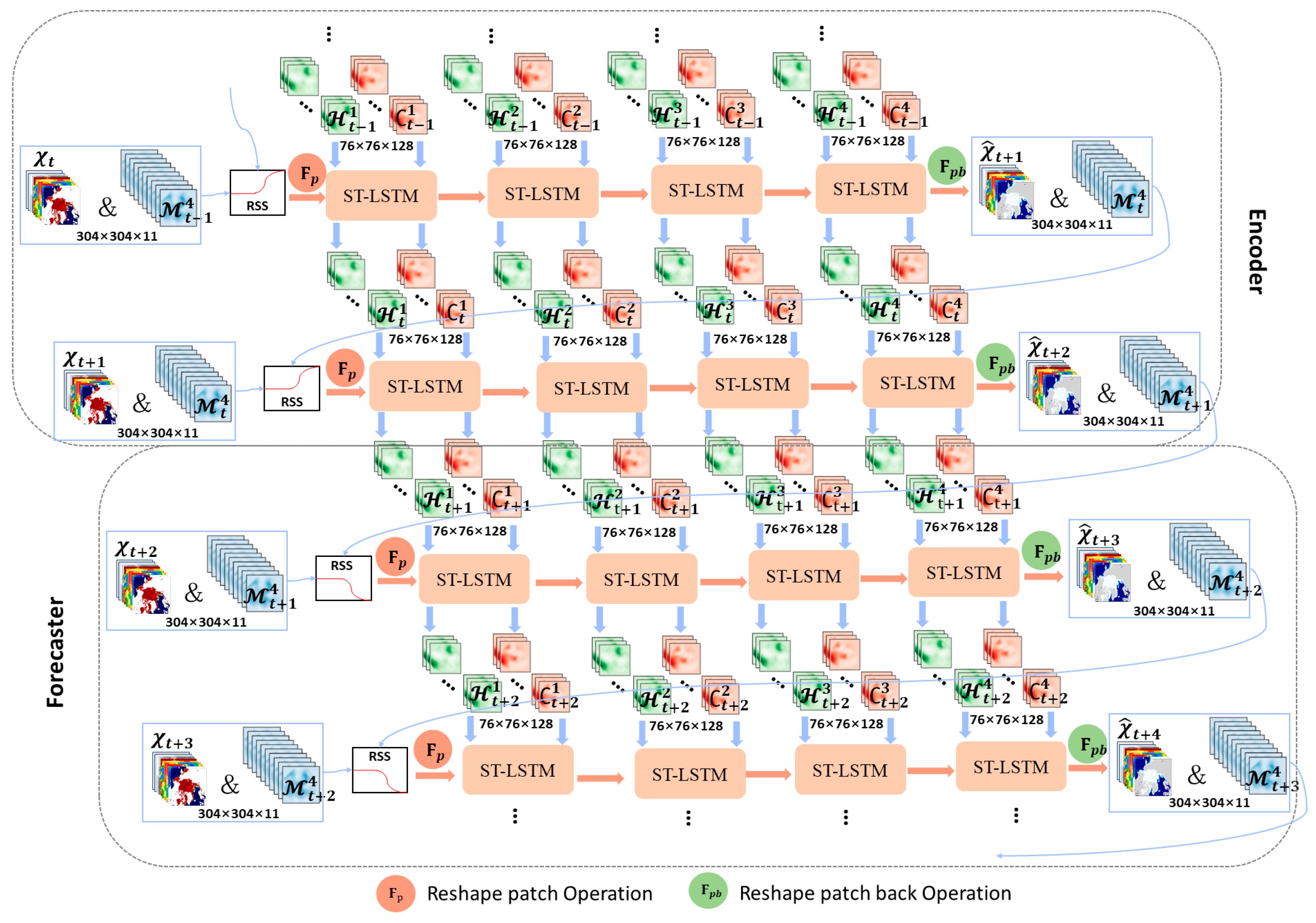
2.2. Models
2.3. Evaluation Metrics
3. Results and Discussion
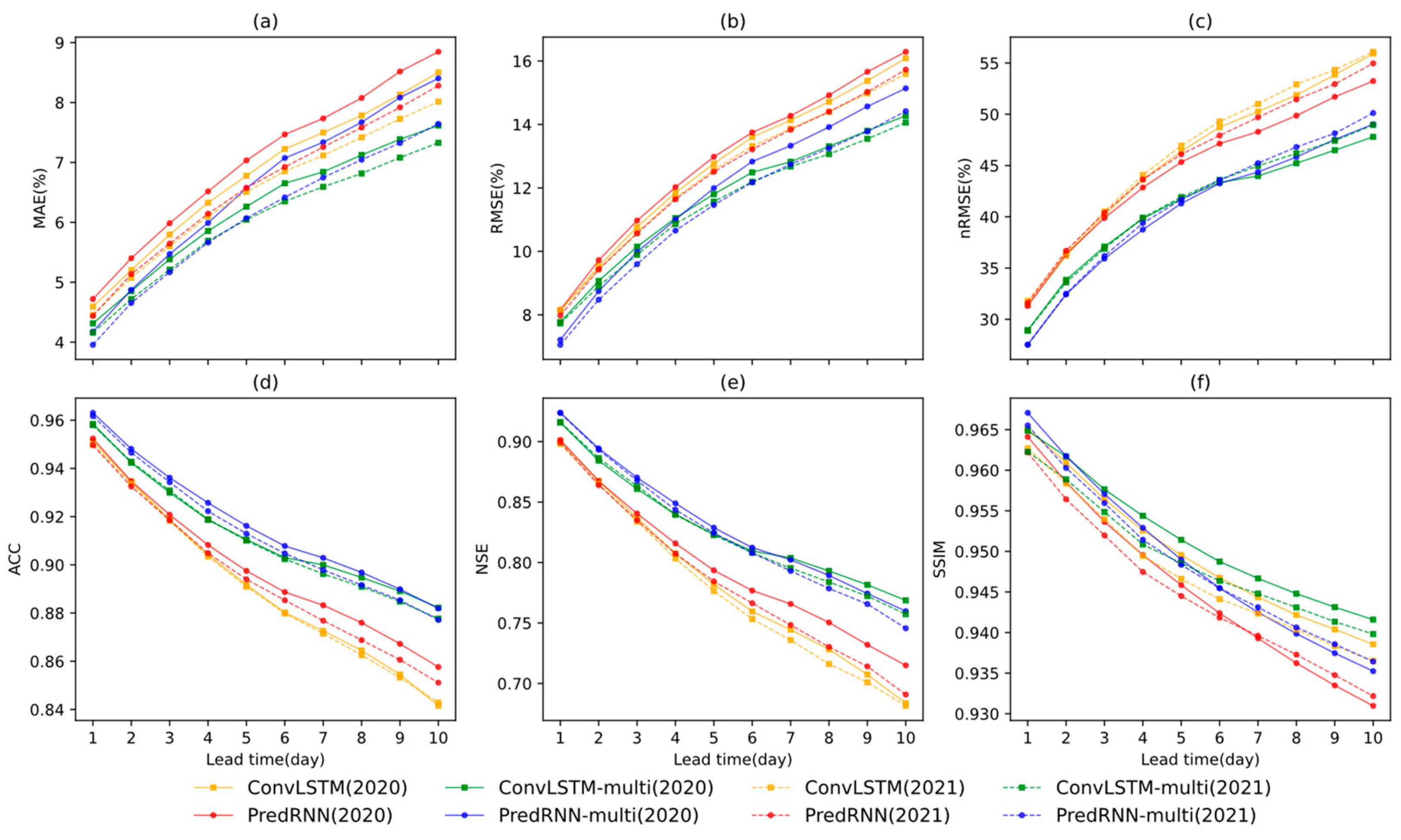
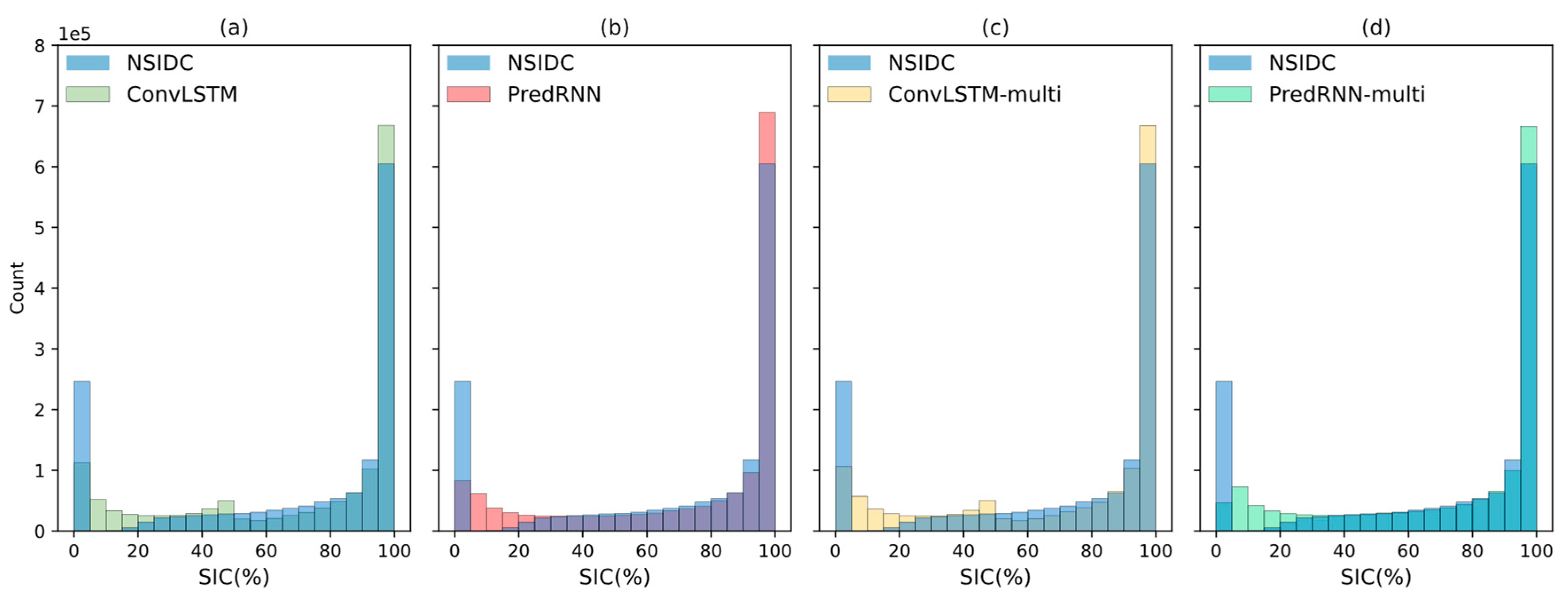
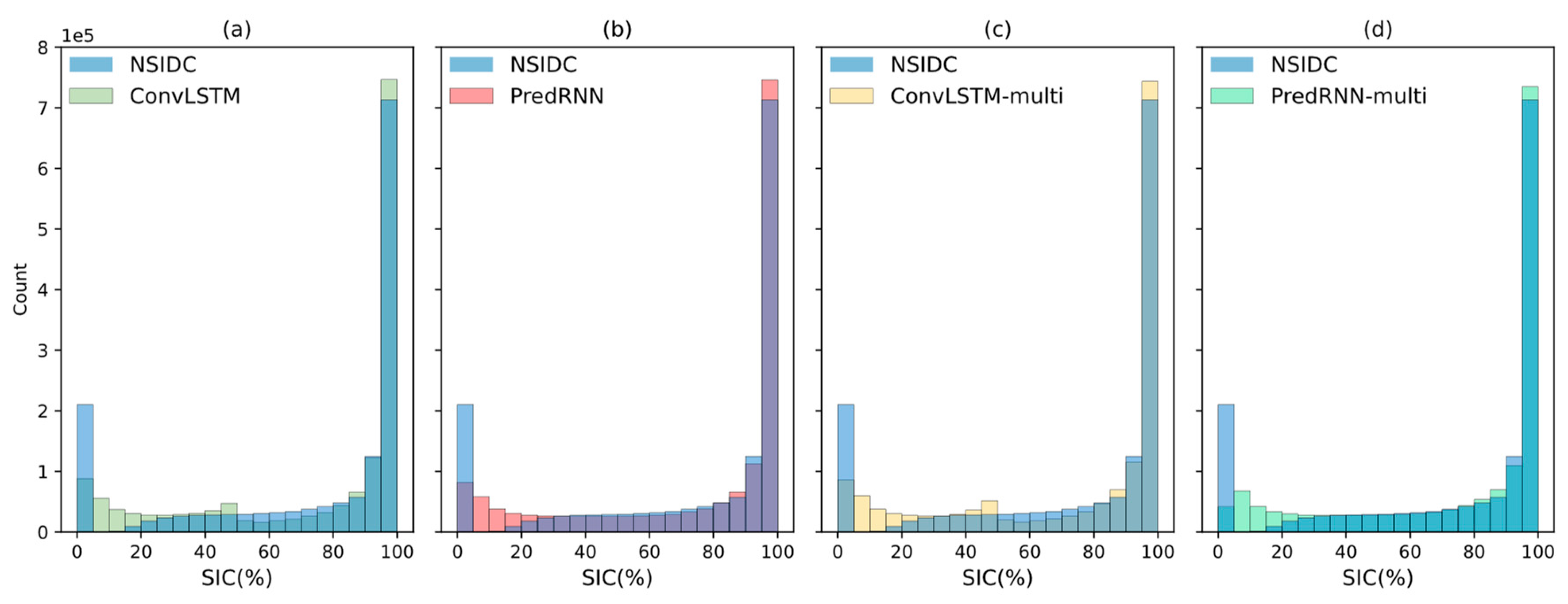
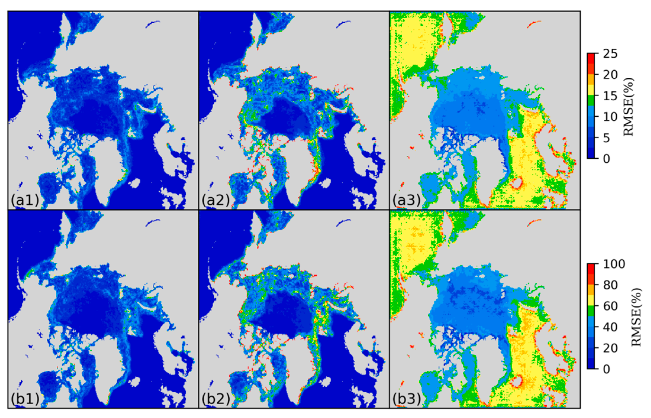
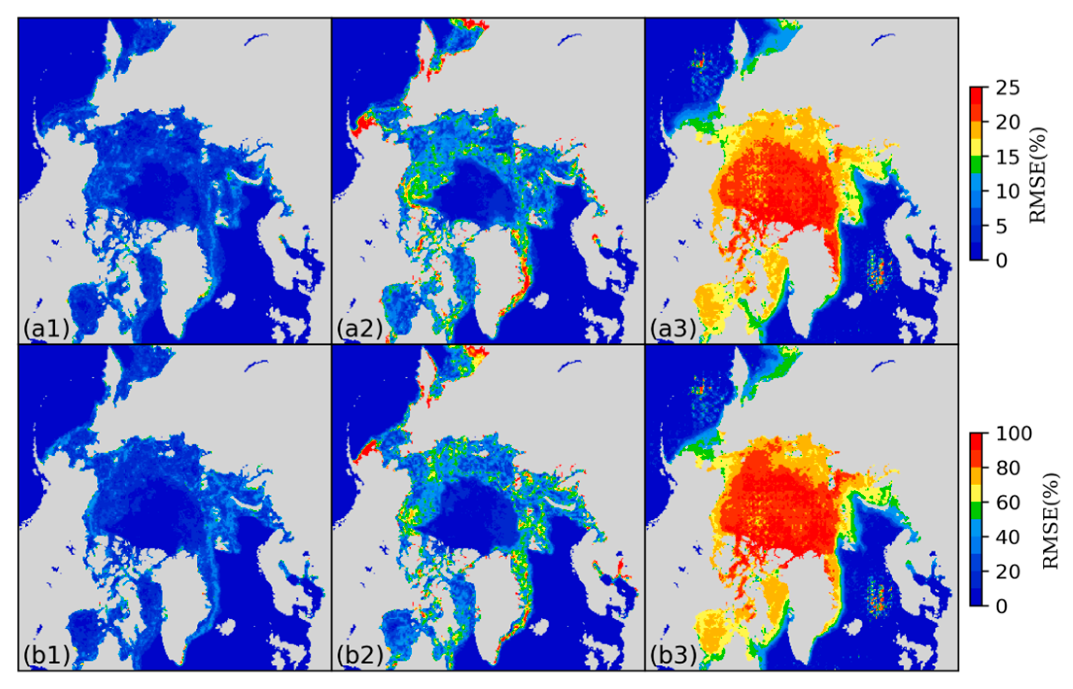
3.1. Daily-Scale Predictions of Sea Ice Concentration
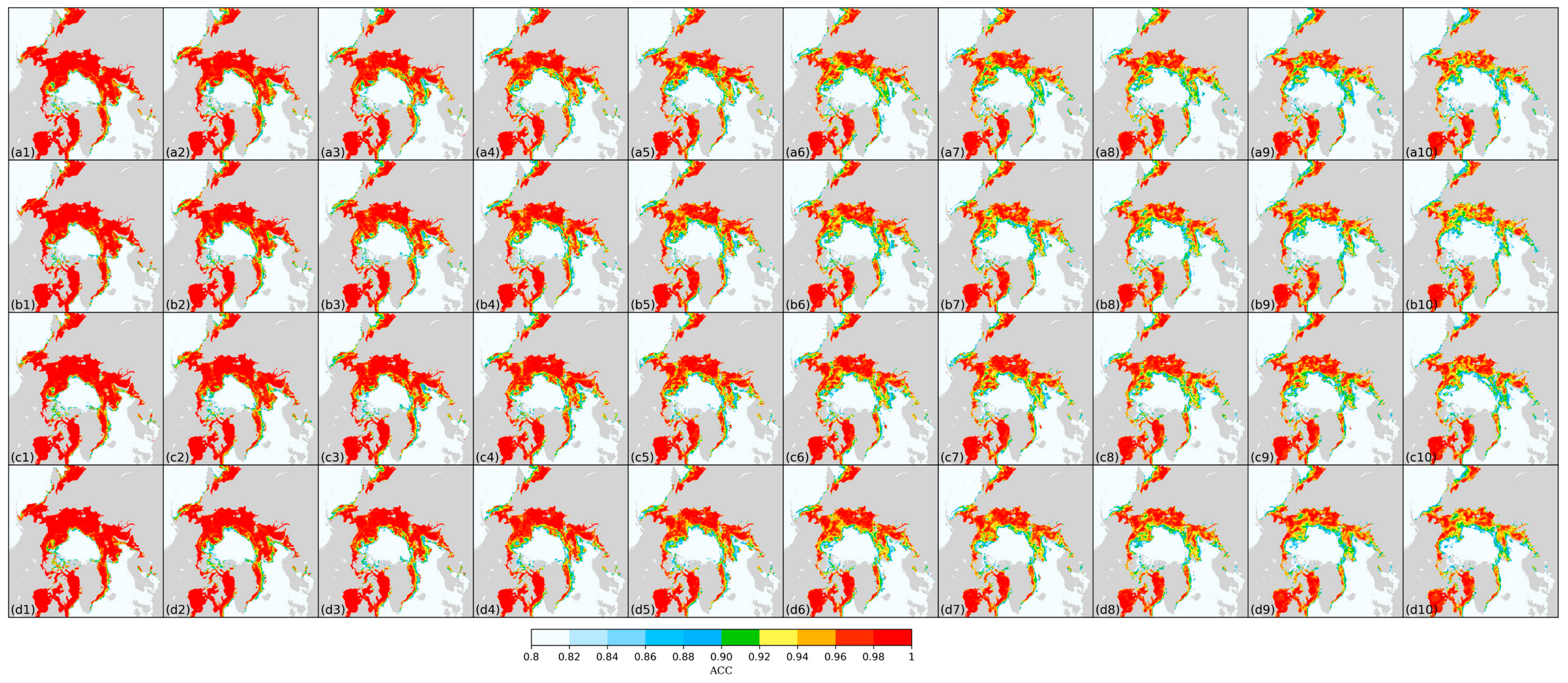
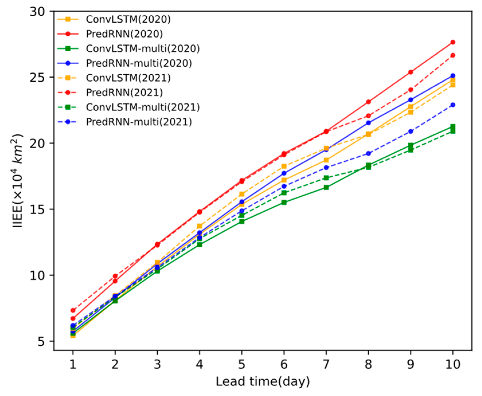
3.2. Sea Ice Edge Prediction Accuracy
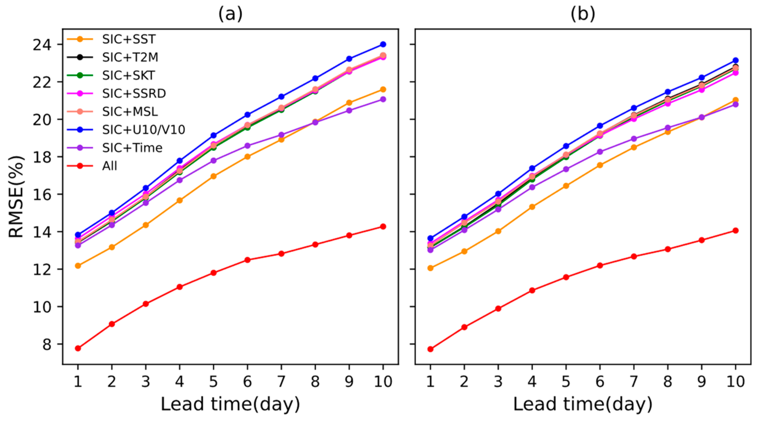
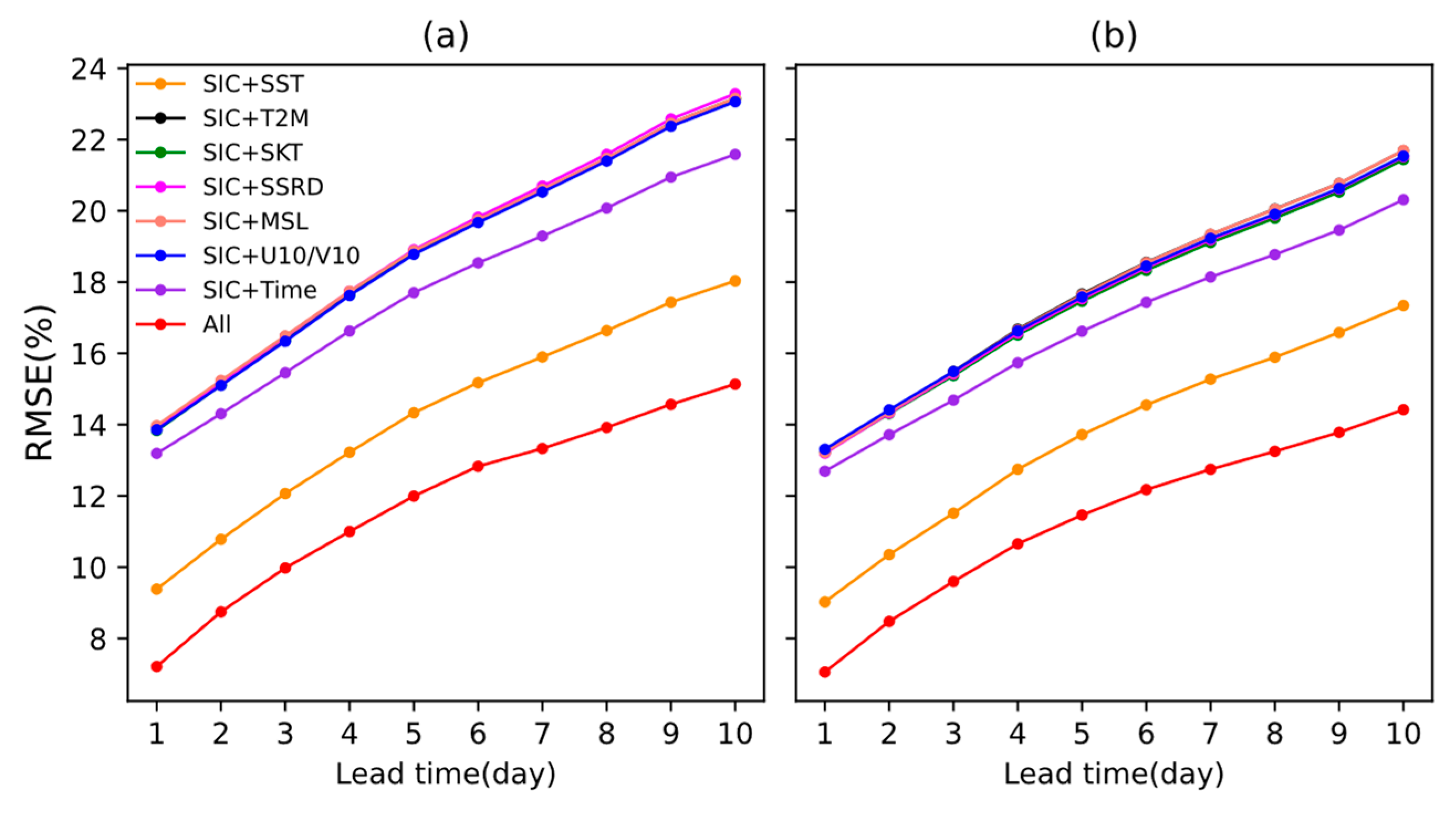
3.3. Parameter Sensitivity Analysis
3.4. Prediction Ability of the Models under Extreme Conditions
4. Conclusions
Author Contributions
Funding
Institutional Review Board Statement
Informed Consent Statement
Data Availability Statement
Conflicts of Interest
Appendix A

| Model | Spatial Resolution | Frequency | Experiment (Ensemble Members) | |||||
|---|---|---|---|---|---|---|---|---|
| ACCESS-CM2 | 360 × 300 | day | SSP126(1) | r1i1p1f1 | SSP245(1) | r1i1p1f1 | SSP585(1) | r1i1p1f1 |
| CESM2-WACCM | 320 × 384 | day | SSP126(1) | r1i1p1f1 | SSP245(5) | r1i1p1f1 | SSP585(5) | r1i1p1f1 |
| r2i1p1f1 | r2i1p1f1 | |||||||
| r3i1p1f1 | r3i1p1f1 | |||||||
| r4i1p1f1 | r4i1p1f1 | |||||||
| r5i1p1f1 | r5i1p1f1 | |||||||
| MIROC6 | 360 × 256 | day | SSP126(3) | r11p1f1 | SSP245(3) | r1i1p1f1 | SSP585(3) | r1i1p1f1 |
| r2i1p1f1 | r2i1p1f1 | r2i1p1f1 | ||||||
| r3i1p1f1 | r3i1p1f1 | r3i1p1f1 | ||||||
| MRI-ESM2-0 | 360 × 364 | day | SSP126(1) | r1i1p1f1 | SSP245(1) | r1i1p1f1 | SSP585(1) | r1i1p1f1 |


References
- Serreze, M.C.; Meier, W.N. The Arctic′s sea ice cover: Trends, variability, predictability, and comparisons to the Antarctic. Ann. N. Y. Acad. Sci. 2019, 1436, 36–53. [Google Scholar] [CrossRef] [PubMed]
- Cavalieri, D.J.; Parkinson, C.L. Arctic sea ice variability and trends, 1979–2010. Cryosphere 2012, 6, 881–889. [Google Scholar] [CrossRef]
- Stroeve, J.C.; Serreze, M.C.; Holland, M.M.; Kay, J.E.; Malanik, J.; Barrett, A.P. The Arctic′s rapidly shrinking sea ice cover: A research synthesis. Clim. Chang. 2012, 110, 1005. [Google Scholar] [CrossRef]
- Devasthale, A.; Sedlar, J.; Koenigk, T.; Fetzer, E. The thermodynamic state of the Arctic atmosphere observed by AIRS: Comparisons during the record minimum sea ice extents of 2007 and 2012. Atmos. Chem. Phys. 2013, 13, 7441–7450. [Google Scholar] [CrossRef]
- Wang, Y.; Bi, H.; Huang, H.; Liu, Y.; Liu, Y.; Liang, X.; Fu, M.; Zhang, Z. Satellite-observed trends in the Arctic sea ice concentration for the period 1979–2016. J. Oceanol. Limnol. 2019, 37, 18–37. [Google Scholar] [CrossRef]
- Simmonds, I.; Li, M. Trends and variability in polar sea ice, global atmospheric circulations, and baroclinicity. Ann. N. Y. Acad. Sci. 2021, 1504, 167–186. [Google Scholar] [CrossRef]
- Witze, A. Arctic Sea Ice Hits Second-Lowest Level on Record. Available online: https://www.nature.com/articles/d41586-020-02705-7 (accessed on 5 July 2023).
- Pizzolato, L.; Howell, S.E.; Derksen, C.; Dawson, J.; Copland, L. Changing sea ice conditions and marine transportation activity in Canadian Arctic waters between 1990 and 2012. Clim. Chang. 2014, 123, 161–173. [Google Scholar] [CrossRef]
- Gascard, J.-C.; Riemann-Campe, K.; Gerdes, R.; Schyberg, H.; Randriamampianina, R.; Karcher, M.; Zhang, J.; Rafizadeh, M. Future sea ice conditions and weather forecasts in the Arctic: Implications for Arctic shipping. Ambio 2017, 46, 355–367. [Google Scholar] [CrossRef] [PubMed]
- Stephenson, S.R.; Pincus, R. Challenges of sea-ice prediction for Arctic marine policy and planning. J. Borderl. Stud. 2018, 33, 255–272. [Google Scholar] [CrossRef]
- Luo, D.; Yao, Y.; Dai, A.; Simmonds, I.; Zhong, L. Increased quasi stationarity and persistence of winter Ural blocking and Eurasian extreme cold events in response to Arctic warming. Part II: A theoretical explanation. J. Clim. 2017, 30, 3569–3587. [Google Scholar] [CrossRef]
- Rudeva, I.; Simmonds, I. Midlatitude winter extreme temperature events and connections with anomalies in the Arctic and tropics. J. Clim. 2021, 34, 3733–3749. [Google Scholar] [CrossRef]
- Luo, B.; Wu, L.; Luo, D.; Dai, A.; Simmonds, I. The winter midlatitude-Arctic interaction: Effects of North Atlantic SST and high-latitude blocking on Arctic sea ice and Eurasian cooling. Clim. Dyn. 2019, 52, 2981–3004. [Google Scholar] [CrossRef]
- Blanchard-Wrigglesworth, E.; Armour, K.C.; Bitz, C.M.; DeWeaver, E. Persistence and inherent predictability of Arctic sea ice in a GCM ensemble and observations. J. Clim. 2011, 24, 231–250. [Google Scholar] [CrossRef]
- Krikken, F.; Hazeleger, W. Arctic energy budget in relation to sea ice variability on monthly-to-annual time scales. J. Clim. 2015, 28, 6335–6350. [Google Scholar] [CrossRef]
- Guemas, V.; Blanchard-Wrigglesworth, E.; Chevallier, M.; Day, J.J.; Deque, M.; Doblas-Reyes, F.J.; Fuckar, N.S.; Germe, A.; Hawkins, E.; Keeley, S.; et al. A review on Arctic sea-ice predictability and prediction on seasonal to decadal time-scales. Q. J. R. Meteorol. Soc. 2016, 142, 546–561. [Google Scholar] [CrossRef]
- Mohammadi-Aragh, M.; Goessling, H.; Losch, M.; Hutter, N.; Jung, T. Predictability of Arctic sea ice on weather time scales. Sci. Rep. 2018, 8, 6514. [Google Scholar] [CrossRef] [PubMed]
- Cruz-García, R.; Guemas, V.; Chevallier, M.; Massonnet, F. An assessment of regional sea ice predictability in the Arctic ocean. Clim. Dyn. 2019, 53, 427–440. [Google Scholar] [CrossRef]
- Onarheim, I.H.; Eldevik, T.; Årthun, M.; Ingvaldsen, R.B.; Smedsrud, L.H. Skillful prediction of Barents Sea ice cover. Geophys. Res. Lett. 2015, 42, 5364–5371. [Google Scholar] [CrossRef]
- Nakanowatari, T.; Xie, J.; Bertino, L.; Matsueda, M.; Yamagami, A.; Inoue, J. Ensemble forecast experiments of summertime sea ice in the Arctic Ocean using the TOPAZ4 ice-ocean data assimilation system. Environ. Res. 2022, 209, 112769. [Google Scholar] [CrossRef]
- Leppäranta, M.; Meleshko, V.P.; Uotila, P.; Pavlova, T. Sea Ice Modelling. In Sea Ice in the Arctic: Past, Present and Future; Johannessen, O.M., Bobylev, L.P., Shalina, E.V., Sandven, S., Eds.; Springer International Publishing: Cham, Switzerland, 2020; pp. 315–387. [Google Scholar]
- Kim, J.; Kim, K.; Cho, J.; Kang, Y.Q.; Yoon, H.-J.; Lee, Y.-W. Satellite-Based Prediction of Arctic Sea Ice Concentration Using a Deep Neural Network with Multi-Model Ensemble. Remote Sens. 2019, 11, 19. [Google Scholar] [CrossRef]
- Fritzner, S.; Graversen, R.; Christensen, K.H. Assessment of High-Resolution Dynamical and Machine Learning Models for Prediction of Sea Ice Concentration in a Regional Application. J. Geophys. Res.-Ocean. 2020, 125, e2020JC016277. [Google Scholar] [CrossRef]
- Kim, Y.J.; Kim, H.C.; Han, D.; Lee, S.; Im, J. Prediction of monthly Arctic sea ice concentrations using satellite and reanalysis data based on convolutional neural networks. Cryosphere 2020, 14, 1083–1104. [Google Scholar] [CrossRef]
- Andersson, T.R.; Hosking, J.S.; Perez-Ortiz, M.; Paige, B.; Elliott, A.; Russell, C.; Law, S.; Jones, D.C.; Wilkinson, J.; Phillips, T.; et al. Seasonal Arctic sea ice forecasting with probabilistic deep learning. Nat. Commun. 2021, 12, 5124. [Google Scholar] [CrossRef] [PubMed]
- Liu, Q.; Zhang, R.; Wang, Y.; Yan, H.; Hong, M. Daily Prediction of the Arctic Sea Ice Concentration Using Reanalysis Data Based on a Convolutional LSTM Network. J. Mar. Sci. Eng. 2021, 9, 330. [Google Scholar] [CrossRef]
- Liu, Y.; Bogaardt, L.; Attema, J.; Hazeleger, W. Extended-Range Arctic Sea Ice Forecast with Convolutional Long Short-Term Memory Networks. Mon. Weather Rev. 2021, 149, 1673–1693. [Google Scholar] [CrossRef]
- Grigoryev, T.; Verezemskaya, P.; Krinitskiy, M.; Anikin, N.; Gavrikov, A.; Trofimov, I.; Balabin, N.; Shpilman, A.; Eremchenko, A.; Gulev, S. Data-driven short-term daily operational sea ice regional forecasting. Remote Sens. 2022, 14, 5837. [Google Scholar] [CrossRef]
- Lin, Y.; Yang, Q.; Li, X.; Yang, C.-Y.; Wang, Y.; Wang, J.; Liu, J.; Chen, S.; Liu, J. Optimization of the k-nearest-neighbors model for summer Arctic sea ice prediction. Front. Mar. Sci. 2023, 10, 1260047. [Google Scholar] [CrossRef]
- Comiso, J.C. Bootstrap Sea Ice Concentrations from Nimbus-7 SMMR and DMSP SSM/I-SSMIS, Version 3. Available online: https://nsidc.org/data/nsidc-0079/versions/3 (accessed on 10 November 2022).
- Hersbach, H.; Bell, B.; Berrisford, P.; Biavati, G.; Horányi, A.; Muñoz Sabater, J.; Nicolas, J.; Peubey, C.; Radu, R.; Rozum, I.; et al. ERA5 Hourly Data on Single Levels from 1940 to Present. Copernicus Climate Change Service (C3S) Climate Data Store (CDS). Available online: https://cds.climate.copernicus.eu/cdsapp#!/dataset/10.24381/cds.adbb2d47?tab=overview (accessed on 10 November 2022).
- Arctic Sea Ice Minimum is 2nd Lowest on Record. Available online: https://public.wmo.int/en/media/news/arctic-sea-ice-minimum-2nd-lowest-record (accessed on 5 July 2023).
- Notz, D.; Community, S. Arctic sea ice in CMIP6. Geophys. Res. Lett. 2020, 47, e2019GL086749. [Google Scholar] [CrossRef]
- Shi, X.J.; Chen, Z.R.; Wang, H.; Yeung, D.Y.; Wong, W.K.; Woo, W.C. Convolutional LSTM Network: A Machine Learning Approach for Precipitation Nowcasting. In Proceedings of the 29th Annual Conference on Neural Information Processing Systems (NIPS), Montreal, QC, Canada, 7–12 December 2015. [Google Scholar]
- Wang, Y.; Wu, H.; Zhang, J.; Gao, Z.; Wang, J.; Yu, P.; Long, M. PredRNN: A Recurrent Neural Network for Spatiotemporal Predictive Learning. IEEE Trans. Pattern Anal. Mach. Intell. 2022, 45, 2208–2225. [Google Scholar] [CrossRef] [PubMed]
- Sutskever, I.; Vinyals, O.; Le, Q.V. Sequence to sequence learning with neural networks. Adv. Neural Inf. Process. Syst. 2014, 27, 3104–3112. [Google Scholar]
- Bengio, S.; Vinyals, O.; Jaitly, N.; Shazeer, N. Scheduled Sampling for Sequence Prediction with Recurrent Neural Networks. In Proceedings of the 29th Annual Conference on Neural Information Processing Systems (NIPS), Montreal, QC, Canada, 7–12 December 2015. [Google Scholar]
- Melsom, A.; Palerme, C.; Müller, M. Validation metrics for ice edge position forecasts. Ocean Sci. 2019, 15, 615–630. [Google Scholar] [CrossRef]
- Melsom, A. Edge displacement scores. Cryosphere 2021, 15, 3785–3796. [Google Scholar] [CrossRef]
- Goessling, H.F.; Tietsche, S.; Day, J.J.; Hawkins, E.; Jung, T. Predictability of the Arctic sea ice edge. Geophys. Res. Lett. 2016, 43, 1642–1650. [Google Scholar] [CrossRef]
- Schauer, U.; Loeng, H.; Rudels, B.; Ozhigin, V.K.; Dieck, W. Atlantic water flow through the Barents and Kara Seas. Deep Sea Res. Part I Oceanogr. Res. Pap. 2002, 49, 2281–2298. [Google Scholar] [CrossRef]
- Årthun, M.; Eldevik, T.; Smedsrud, L.; Skagseth, Ø.; Ingvaldsen, R. Quantifying the influence of Atlantic heat on Barents Sea ice variability and retreat. J. Clim. 2012, 25, 4736–4743. [Google Scholar] [CrossRef]
- Luo, B.; Luo, D.; Ge, Y.; Dai, A.; Wang, L.; Simmonds, I.; Xiao, C.; Wu, L.; Yao, Y. Origins of Barents-Kara sea-ice interannual variability modulated by the Atlantic pathway of El Niño–Southern Oscillation. Nat. Commun. 2023, 14, 585. [Google Scholar] [CrossRef]
- Pfirman, S.; Colony, R.; Nürnberg, D.; Eicken, H.; Rigor, I. Reconstructing the origin and trajectory of drifting Arctic sea ice. J. Geophys. Res. Ocean. 1997, 102, 12575–12586. [Google Scholar] [CrossRef]
- Pavlov, V.; Pavlova, O.; Korsnes, R. Sea ice fluxes and drift trajectories from potential pollution sources, computed with a statistical sea ice model of the Arctic Ocean. J. Mar. Syst. 2004, 48, 133–157. [Google Scholar] [CrossRef]
- Chevallier, M.; y Mélia, D.S.; Voldoire, A.; Déqué, M.; Garric, G. Seasonal forecasts of the pan-Arctic sea ice extent using a GCM-based seasonal prediction system. J. Clim. 2013, 26, 6092–6104. [Google Scholar] [CrossRef]


| Variable | Source | Unit | Temporal Resolution | Spatial Resolution | Value Range |
|---|---|---|---|---|---|
| Sea ice concentration | NSIDC | % | Daily | 25 km | [0, 1] |
| Sea surface temperature | ECMWF ERA5 | K | Hourly | 0.25° | [0, 1] |
| 2m temperature | ECMWF ERA5 | K | Hourly | 0.25° | [0, 1] |
| Skin temperature | ECMWF ERA5 | K | Hourly | 0.25° | [0, 1] |
| Surface solar radiation downwards | ECMWF ERA5 | J m−2 | Hourly | 0.25° | [0, 1] |
| Mean sea level pressure | ECMWF ERA5 | Pa | Hourly | 0.25° | [0, 1] |
| 10m u-component of wind | ECMWF ERA5 | m s−1 | Hourly | 0.25° | [0, 1] |
| 10m v-component of wind | ECMWF ERA5 | m s−1 | Hourly | 0.25° | [0, 1] |
| Land mask | # | # | Daily | 25 km | 0/1 |
| Cosine of initialization day index | # | # | Daily | 25 km | [−1, 1] |
| Sine of initialization day index | # | # | Daily | 25 km | [−1, 1] |
| Year | Scenarios | MAE | RMSE | nRMSE | ACC | NSE |
|---|---|---|---|---|---|---|
| 2020 | SSP126 | 19.67% | 29.13% | 69% | 0.76 | 0.53 |
| SSP245 | 23.57% | 32.94% | 78% | 0.74 | 0.47 | |
| SSP585 | 25.44% | 35.2% | 85% | 0.71 | 0.41 | |
| 2021 | SSP126 | 20.08% | 29.22% | 70% | 0.76 | 0.53 |
| SSP245 | 23.32% | 32.11% | 76% | 0.75 | 0.49 | |
| SSP585 | 24.58% | 33.95% | 80% | 0.73 | 0.45 |
| ConvLSTM | PredRNN | ConvLSTM-Multi | PredRNN-Multi | SSP126 | SSP245 | SSP585 | ||||||||
|---|---|---|---|---|---|---|---|---|---|---|---|---|---|---|
| WS | SA | WS | SA | WS | SA | WS | SA | WS | SA | WS | SA | WS | SA | |
| 5.44 | 14.97 | 6.28 | 18.10 | 5.45 | 15.51 | 5.05 | 16.86 | 30.50 | 127.46 | 28.74 | 203.26 | 30.85 | 217.10 | |
| 5.03 | 12.51 | 5.15 | 13.72 | 4.87 | 11.74 | 4.79 | 13.52 | 25.18 | 90.62 | 23.32 | 124.80 | 23.36 | 132.34 | |
| 1.42 | 4.70 | 1.68 | 5.68 | 1.55 | 4.39 | 1.36 | 7.73 | 6.92 | 66.94 | 2.62 | 111.80 | 3.54 | 118.79 | |
| 1.07 | 1.22 | 1.19 | 1.27 | 1.10 | 1.31 | 1.05 | 1.23 | 1.22 | 1.4 | 1.24 | 1.54 | 1.33 | 1.56 | |
Disclaimer/Publisher’s Note: The statements, opinions and data contained in all publications are solely those of the individual author(s) and contributor(s) and not of MDPI and/or the editor(s). MDPI and/or the editor(s) disclaim responsibility for any injury to people or property resulting from any ideas, methods, instructions or products referred to in the content. |
© 2023 by the authors. Licensee MDPI, Basel, Switzerland. This article is an open access article distributed under the terms and conditions of the Creative Commons Attribution (CC BY) license (https://creativecommons.org/licenses/by/4.0/).
Share and Cite
Feng, J.; Li, J.; Zhong, W.; Wu, J.; Li, Z.; Kong, L.; Guo, L. Daily-Scale Prediction of Arctic Sea Ice Concentration Based on Recurrent Neural Network Models. J. Mar. Sci. Eng. 2023, 11, 2319. https://doi.org/10.3390/jmse11122319
Feng J, Li J, Zhong W, Wu J, Li Z, Kong L, Guo L. Daily-Scale Prediction of Arctic Sea Ice Concentration Based on Recurrent Neural Network Models. Journal of Marine Science and Engineering. 2023; 11(12):2319. https://doi.org/10.3390/jmse11122319
Chicago/Turabian StyleFeng, Juanjuan, Jia Li, Wenjie Zhong, Junhui Wu, Zhiqiang Li, Lingshuai Kong, and Lei Guo. 2023. "Daily-Scale Prediction of Arctic Sea Ice Concentration Based on Recurrent Neural Network Models" Journal of Marine Science and Engineering 11, no. 12: 2319. https://doi.org/10.3390/jmse11122319
APA StyleFeng, J., Li, J., Zhong, W., Wu, J., Li, Z., Kong, L., & Guo, L. (2023). Daily-Scale Prediction of Arctic Sea Ice Concentration Based on Recurrent Neural Network Models. Journal of Marine Science and Engineering, 11(12), 2319. https://doi.org/10.3390/jmse11122319