Adaptive Fuzzy Quantized Control for a Cooperative USV-UAV System Based on Asynchronous Separate Guidance

Abstract

This paper focuses predominantly on the multi-tasks carried out by the cooperative unmanned surface vehicle-unmanned aerial vehicle (USV-UAV) system in which the input quantization is considered. The proposed cooperative scheme consists of the asynchronous separate guidance and adaptive fuzzy quantized control algorithm. The proposed guidance law takes full advantage of subsystems whilst considering the maneuverability of these subsystems in order to achieve the goal of executing multi-tasks. In contrast to previous guidance laws, although the same waypoint path is planned, the calculation for guidance law proposed is based on speed rather than time, which in reality is more relevant. As for the controls, an adaptive fuzzy quantized controller was developed to reduce undue exertion on the actuator. By fusing the dynamic surface control (DSC) and fuzzy logic system (FLS), a hysteresis quantizer has been introduced to reduce the transmission load. By properly adjusting the quantization density, the number of quantizations was reduced whilst maintaining a favorable control performance. All of the stated variables are semi-global uniform ultimate bounded (SGUUB) and the stability of the USV-UAV system is proofed through the Lyapunov theorem. Finally, the advantages of the proposed scheme are evaluated by two simulative experiments, exhibiting the favorable tracking accuracy and reduced wear on the actuators.

1. Introduction

Recently, with the rapid emergence of unmanned surface vehicles (USVs), unmanned aerial vehicles (UAVs) [1] and autonomous underwater vehicles (AUVs) [2], the intelligent unmanned systems which they consist of are gradually emerging.

Although each subsystem has the capability of handling most tasks, when they encounter particularly complicated tasks, intelligent unmanned systems are better suited for these applications. For example, the USV-UAV system has greatly expanded exploration range of whist maintaining endurance, however it can significantly increase its rapidity and efficiency in terms of maritime supervision, exploration, and search and rescue [3,4,5,6,7]. Collaborative coordination of heterogeneous unmanned systems during the execution of a mission is challenging due to the complexity of the environments and the potential for various external disturbances [8,9]. Therefore, it is crucial to refine high-performance algorithms for the USV-UAV collaborative system in order to fully leverage the subsystem.

The guidance term and the control term are significant elements when considering the control of the USV-UAV system. The guidance term is designed to generate reference signals for the USV-UAV system, for which the following guidance methods are commonly used: line-of-sight (LOS), artificial potential field (APF), leader-follower, etc. In [10], the LOS guidance principle is approached as a conventional way that marine vessels adhere to their intended course through a series of waypoints, which ensures proximity is maintained. However, LOS-related methods solely concentrate on the tracking precision of straight lines and exhibit inadequate performance in path planning around curves. In [11], an improved dynamic virtual ship (DVS) guidance principle is proposed. The DVS can be used as a complementary reference model that not only provides improved performance in curves, but is also more relevant in practice. The aforementioned approach is dependent on time and may generate cumulative errors which decreases the precision if the guidance path is overly intricate. In the realm of cooperative USV-UAV system, comparable guidance methods are used. Based on the LOS guidance principle, a revised 3-dimensional (3D) mapping guidance was developed to ensure that the UAV flies with the USV [12]. The reference signals of the USV and the UAV are simultaneous in order to guarantee their accompaniment. In [13], a novel guidance law based on the combination of virtual structure and APF was proposed for the USV-UAV system. However, when facing complex situations, the APF method exhibits poor performance as the multiple potential fields can affect each other. In order to solve the problem of cooperative path planning for a multi-target air-sea heterogeneous unmanned system, a trans-regional cooperative control model is established [14]. However, the path planning in this paper does not sufficiently take into account the turns nor is it practical enough. In [15], a two-phase landing method was proposed for landing the UAV on the USV precisely using standard GPS and an IR beacon. The guidance section is comprised of the accompanying flight segment and the landing segment. The test results demonstrate that the landing error falls within the range of 20 cm. However, as for the approach to ports, a different method was applied. In [16], a clustering-based approach is adopted, which involves identifying ship trajectories of different patterns of motion corresponding to in-port and out-port ship routes based on Principal Component Analysis and K-mean clustering algorithms. As for the control term, numerous methods were used in the USV-UAV system, such as robust adaptive neural control [17], fuzzy logic system (FLS) [12], particle swarm optimization (PSO) [18], prescribed performance control (PPC) [19,20], event-triggered control (ETC) [21], sliding mode control [22], etc. The aforementioned literatures predominantly concentrate on the autonomous navigation guidance and control of single agents. As for multi-agents, the guidance principle in the aforementioned studies may not be sufficiently practical or they could fail to fully exploit the advantages of the USV-UAV system.

Currently, a selection of high-performance control algorithms is proposed for the hetero-class system. The issues in achieving an accurate attitude tracking control for quadrotor UAVs was successfully solved by merging the tracking differentiator and the extended state observer strategies as described in [23]. In order to avoid an “explosion of complexity”, the dynamic surface control (DSC) technique [24], which is a first-order filter for virtual control signals, was introduced so as to avoid the high computational burden. In contrast to the formations of USVs or UAVs, which are homogeneous, the cooperative USV-UAV system is of mixed order. Despite this, comparable issues such as model uncertainties [25], external disturbances [26], input constraints [27], and communication burden [28] must be addressed in the control section. A learning-based adaptive robust control (LARC) framework is proposed in [29] to tackle the parametric and nonlinear uncertainties which are influenced by a varying environment. The position and attitude signals in the control of the USV-UAV system are generated by the computer, then transmitted via the communication channel, whereby they are quantized before passing again through the communication channel. Thus, quantized control is introduced which guarantees a certain closed-loop performance whilst requiring low communication rates and addressing uncertainties. In [30], an adaptive quantized control strategy was proposed for linear uncertain systems based on Lyapunov theory. In [31], focusing on nonlinear uncertain systems with quantized input, an enhanced adaptive control scheme with a new hysteretic quantizer was developed. The introduced hysteretic quantizer can avoid the oscillation caused by the logarithmic quantizer. A backstepping-based adaptive stabilization method was devised for parametric strict-feedback systems featuring hysteretic quantization in [32]. In [33], a composite adaptive quantized controller was constructed based on the DSC technique for UAV. In [34], a new collaborative platform between USV and UAV was introduced, providing a solid basis for cooperative tasks performed by the combined USV-UAV systems. In [35], an improved PSO algorithm aimed to form cooperative path planning for the air-sea heterogeneous vehicles. Most of the results in the corresponding literatures solely pertain to the control design for systems of identical order. However, as for USV-UAV systems with heterogeneous properties, there is a lack of research that focuses on quantized stabilization, however, in spite of this problem, tracking quantized feedback has greater practical significance.

For ensuring the proper operation of the guidance algorithm and its compatibility with marine engineering applications, a control algorithm has been designed which has the superiority to the concise form and less actuator wear. The main contributions in this paper can be summarized in the following two aspects:

(1) For the cooperative USV-UAV system, an asynchronous separate guidance principle has been developed to perform multiple tasks within a designed timeframe. In contrast to [10], the proposed guidance principle effectively utilizes subsystems in complicated scenarios. As for the application of multi-tasks, the proposed guidance principle applies to the USV-UAV system and has an improved performance to homogeneous systems, which consist of single USVs or UAVs. Notably, as with the waypoint-based route described in [11,13], the curved line is a circular arc which is calculated based on a fixed pre-set velocity, but the proposed guidance principle calculates the path of the curved line based on the velocity and the distance between the vessel and the target point, which is more relevant to the actual context.

(2) A novel adaptive fuzzy quantized control strategy for the USV-UAV system is presented. The continuous input signal is segmented into suitable fixed-value segments through the implementation of hysteresis quantization, which causes a significant reduction in transmission load and wear of the actuator. Furthermore, additional parameters are designated to eliminate the adverse effect induced by inconsistencies caused by the heterogenous model of ship.

The remainder of this paper is organized as follows. In Section 2, the problem formulation and preliminaries are presented. In Section 3 and Section 4, we give a systematic procedure for the control design. In Section 5, numerical simulations and comparative experiments are provided. Finally, Section 6 concludes this paper.

2. Problem for Formulation and Preliminaries

In Section 2, the following three parts are proposed for further analysis. Section 2.1 introduces the model of mix-ordered USV-UAV system, Section 2.2 presents the FLS, and Section 2.3 demonstrates the basic principle of the hysteresis quantization.

2.1. USV-UAV System Modeling

According to [11,36,37], the nonlinear dynamic model of USV-UAV systems can be expressed as:

$$\left\{\begin{array}{l}{\dot{x}}_s=u_{au}\cos \left({\psi }_s\right)-v_s\sin \left({\psi }_s\right)\\ {\dot{y}}_s=u_{au}\sin \left({\psi }_s\right)+v_s\cos \left({\psi }_s\right)\\ {\dot{\psi }}_s=r_{ar}\\ {\dot{x}}_a=u_{ax},{\dot{y}}_a=u_{ay},{\dot{z}}_a=u_{az}\\ {\dot{\varphi }}_a=r_{a\varphi },{\dot{\theta }}_a=r_{a\theta },{\dot{\psi }}_a=r_{a\psi }\end{array}\right.$$

(1)

$$\left\{\begin{array}{l}\stackrel{.}{u_{au}}=\frac{m_v}{m_u}\cdot v_s{r}_{ar}-f_u\left({\nu }_s\right)+\frac{{\tau }_u(\cdot )}{m_u}+\frac{d_{wu}}{m_u}\hfill \\ \stackrel{.}{v_s}=-\frac{m_u}{m_v}\cdot u_{au}{r}_{ar}-\frac{f_v\left({\nu }_s\right)}{m_v}+\frac{d_{wv}}{m_v}\hfill \\ \stackrel{.}{r_s}=\frac{\left(m_u-m_v\right)}{m_u}\cdot u_{ar}{v}_s-\frac{f_r(v_s)}{m_r}+\frac{{\tau }_r(\cdot )}{m_r}+\frac{d_{wr}}{m_r}\hfill \\ \stackrel{.}{u_{ax}}=f_x({\nu }_a)+\frac{1}{m}{R}_x{F}_f+d_{wx}\hfill \\ \stackrel{.}{u_{ay}}=f_y({\nu }_a)+\frac{1}{m}{R}_y{F}_f+d_{wy}\hfill \\ \stackrel{.}{u_{az}}=f_z({\nu }_a)+\frac{1}{m}{R}_z{F}_f-g+d_{wz}\hfill \\ {\dot{r}}_{a\varphi }=f_{\varphi }\left({\nu }_a\right)+\frac{d}{I_{xx}}{\tau }_{\psi }+d_{w\varphi }\hfill \\ {\dot{r}}_{a\theta }=f_{\theta }\left({\nu }_a\right)+\frac{d}{I_{yy}}{\tau }_{\varphi }+d_{w\theta }\hfill \\ {\dot{r}}_{a\psi }=f_{\psi }\left({\nu }_a\right)+\frac{1}{I_{zz}}{\tau }_{\theta }+d_{w\psi }\hfill \end{array}\right.$$

(2)

where ${\left[x_j,y_j,z_a,{\psi }_j,{\varphi }_j,{\theta }_j\right]}^{\mathrm{T}},j=s,a$ describe the surge, sway, heaving displacement, yaw, roll, and pitch angle for the USV-UAV system. ${\mathit{v}}_s={\left[u_{au},v_s,r_{ar}\right]}^T$ represent the surge, sway, and yaw velocities of the USV. ${\mathit{v}}_a={\left[u_{ax},u_{ay},u_{az},r_{a\varphi },r_{a\theta },r_{a\psi }\right]}^{\mathrm{T}}$ are the velocities and the rotational velocities along the x-axis, y-axis, and z-axis in the body-fixed frame of the UAV. $m_u,m_v,m_r$ indicate the additional mass of the USV in three considered orientations.${\tau }_u,{\tau }_r,{\tau }_{\psi },{\tau }_{\varphi },{\tau }_{\theta }$ are the surge force and the yaw moment of the USV and the rotational moments for the roll, pitch, and yaw angle of the UAV. $m$ is the mass of the UAV and $g$ is the gravitational acceleration. $I_{xx},I_{yy},I_{zz}$ describe the rotary inertia. $d_{wk},k=u,v,r,x,y,z,\psi ,\varphi ,\theta$ denote the external disturbances originating from different directions. The total force $F_f$ acting on $F_i,i=1,2,3,4$ is generated by the four propellers of the UAV (see Figure 1). $R_x,R_y,R_z$ are the attitude matrix. $d$ is the diagonal diameter of the UAV, considering $d_{u1},d_{u2},d_{u3},d_{v1},d_{v2},d_{v3},d_{r1},d_{r2},d_{r3}$ are all regarded as unknown parameters and describe the nonlinear damping terms. $k_{dx},k_{dy},k_{dz}$ denote the translation drag coefficients $f_u({\mathit{v}}_s),f_v({\mathit{v}}_s),f_r({\mathit{v}}_s)$ and $f_x({\mathit{v}}_a),f_y({\mathit{v}}_a),f_z({\mathit{v}}_a),f_{\varphi }({\mathit{v}}_a),f_{\theta }({\mathit{v}}_a),$$f_{\psi }({\mathit{v}}_a)$ are the respective nonlinear functions of the UAV and USV, presented as follows.

$$\left\{\begin{array}{l}{f}_u({\mathit{v}}_s)=d_{u1}{u}_{au}+d_{u2}\left|u_{au}\right|u_{au}+d_{u3}{u}_{au}^3\hfill \\ f_v({\mathit{v}}_s)=d_{v1}{v}_s+d_{v2}\left|v_s\right|v_s+d_{v3}{v}_s^3\hfill \\ f_r({\mathit{v}}_s)=d_{r1}{r}_{ar}+d_{r2}\left|r_{ar}\right|r_{ar}+d_{r3}{r}_{ar}^3\hfill \\ f_x({\mathit{v}}_a)=-\frac{k_{dx}}{m}{u}_{ax},f_y({\mathit{v}}_a)=-\frac{k_{dy}}{m}{u}_{ay},f_z({\mathit{v}}_a)=-\frac{k_{dz}}{m}{u}_{az}\hfill \\ f_{\varphi }({\mathit{v}}_a)=\frac{I_{yy}-I_{zz}}{I_{xx}}\stackrel{.}{{\theta }_a}\stackrel{.}{{\psi }_a}-\frac{{\omega }_r{J}_r}{I_{xx}}\stackrel{.}{{\theta }_a}-\frac{k_{ax}}{I_{xx}}\stackrel{.}{{\varphi }_a{}^2}\hfill \\ f_{\theta }({\mathit{v}}_a)=\frac{I_{zz}-I_{xx}}{I_{yy}}\stackrel{.}{{\varphi }_a}\stackrel{.}{{\psi }_a}+\frac{{\omega }_r{J}_r}{I_{yy}}\stackrel{.}{{\varphi }_a}-\frac{k_{ay}}{I_{yy}}\stackrel{.}{{\theta }_a{}^2}\hfill \\ f_{\psi }({\mathit{v}}_a)=\frac{I_{xx}-I_{yy}}{I_{zz}}\stackrel{.}{{\theta }_a}\stackrel{.}{{\varphi }_a}-\frac{k_{az}}{I_{xx}}\stackrel{.}{{\psi }_a{}^2}\hfill \end{array}\right.$$

(3)

Assumption 1.

One assumes that the external disturbances include the marine disturbances for the USV and the wind disturbance for the UAV. It is assumed that the external disturbance terms satisfy $\left|d_{wk}\right|\le {\overline{d}}_{wk}$, where ${\overline{d}}_{wk}$ are all the positive unknown constants.

Assumption 2.

According to the description in [38], the sway velocity $\mathit{v}$ of the USV is passive-bounded.

Assumption 3.

The UAV possesses symmetry. The rotor speeds vary proportionally to the UAV’s thrust and drag.

Assumption 4.

Throughout this paper, $\left|N\right|$ donates the absolute value of $N$. $\widehat{N}$ donates the estimated value of $N$ and the estimation error $\tilde{N}=\widehat{N}-N$. $‖N‖$ denotes the Euclidean norm of a vector.

Remark 1.

For consistency and clarity, all the time dependence $(t)$ of the time-dependent variables have been omitted from this paper.

2.2. Fuzzy Logic System

In this paper, a fuzzy logic system will be used to approximate $F(x)$ which is a continuously defined function on a compact set $\mathrm{\Omega }$. The fuzzy rules were applied using singleton fuzzifier, product inference, and center-average defuzzifier and they are as follows: If $x_1$ is $F_1^l$ and … and $x_n$ is $F_n^l$; then y is $G^l$, $l=$ 1,2,…,$N$, where $x_i={[x_1,x_2,\dots ,x_n]}^T\in ℝ$ and $y\in \mathrm{R}$ are the input and the output of the fuzzy system. ${\mu }_{F_k^l}$ represents the membership function of fuzzy set $F_n^l$ and $N$ is the number of the rules. Through the use of the singleton function, center-average defuzzification, and product inference, the output of the fuzzy system can be described as

$$y=\frac{{\Sigma }_{l=1}^m{\theta }_l{\mathrm{\Pi }}_{k=1}^n{\mu }_{F_k^l}\left(x_i\right)}{{\Sigma }_{l=1}^m{\mathrm{\Pi }}_{k=1}^n{\mu }_{F_k^l}\left(x_i\right)}={\mathit{\omega }}^T\phi \left(x_i\right)$$

(4)

$\mathit{\omega }={[{\omega }_1,{\omega }_2,\dots ,{\omega }_N]}^T$ is a weight vector and $\mathit{\phi }\left(x_i\right)={[{\phi }_1\left(x\right),{\phi }_2\left(x\right),\dots ,{\phi }_N\left(x\right)]}^T$ is a fuzzy basis vector

$${\mathit{\phi }}_l\left(\mathit{x}\right)=\frac{{\mathrm{\Pi }}_{k=1}^n{\mu }_{F_k^l}\left(x_i\right)}{{\Sigma }_{l=1}^m{\mathrm{\Pi }}_{k=1}^n{\mu }_{F_k^l}\left(x_i\right)},i=1,2,\dots ,m$$

(5)

Lemma 1.

For any given real continuous function $F\left(x\right)$ with $F\left(0\right)=0$, defined in a compact set $\mathrm{\Omega }\in {ℝ}^m$. Then, there exists a FLS such that

$$sup|{\mathit{\omega }}^T{\mathit{\phi }}_l\left({\mathit{x}}_i\right)-F\left({\mathit{x}}_i\right)|\le \epsilon , \forall \epsilon \in \mathrm{\Omega }$$

(6)

where $sup$ is the supremum of the set, ${\mathit{\omega }}^T={\left[{\omega }_1,{\omega }_2,\dots ,{\omega }_m\right]}^T$ is the optimal weight vector with $m>1$ being the number of the fuzzy rules. ${\mathit{\phi }}_l\left({\mathit{x}}_i\right)$ is the fuzzy membership function chosen to be the Gaussian basis function which takes the following form, and $\epsilon$ is the approximation error constant with an unknown upper bound $\overline{\epsilon }$.

$${\mathit{\phi }}_i\left({\mathit{x}}_i\right)=\exp \left(-\frac{{\left(\mathit{x}-{\mathit{\mu }}_i\right)}^T\left(\mathit{x}-{\mathit{\mu }}_i\right)}{2{\xi }_i^2}\right), i=1,2,\dots ,l$$

(7)

where ${\mathit{\mu }}_i$ denotes the center of receptive field and ${\xi }_i$ denotes the standard deviation of the Gaussian function.

2.3. Hysteresis Quantization

In this section, the hysteresis quantizer is used to modify the input signals of the control system. The mathematical model can be described as follows:

$$Q(ti)=\left\{\begin{array}{ll}{u}_{ti}sign(u_{ti})\hfill & \begin{array}{c}{u}_{ti}/(1+\hslash )<\left|u_{ti}\right|\le u_{ti},\dot{u}<0,or\begin{array}{cc}& \end{array}\\ u_{ti}<\left|u_{ti}\right|\le u_{ti}/(1-\hslash ),\dot{u}>0\begin{array}{ccc}& & \end{array}\end{array}\hfill \\ u_{ti}(1+\hslash )sign(u_{ti})\hfill & \begin{array}{c}{u}_{ti}<\left|u_{ti}\right|\le u_{ti}/(1-\hslash ),\dot{u}<0,or\begin{array}{ccc}& & \end{array}\hfill \\ u_{ti}/1-\hslash <\left|u_{ti}\right|\le u_{ti}(1+\hslash )/(1-\hslash ),\dot{u}>0\hfill \end{array}\hfill \\ 0\hfill & \begin{array}{c}0<\left|u_{ti}\right|\le u_{tiMin}/(1+\hslash ),\dot{u}<0,or\\ u_{tiMin}/(1+\hslash )\le \left|u_{ti}\right|\le u_{tiMin},\dot{u}>0\hfill \end{array}\hfill \\ Q(t{i}^{-})\hfill & \begin{array}{cc}\mathrm{other}& \mathrm{cases}\end{array}\hfill \end{array}\right.$$

(8)

where $u_{ti}={\rho }^{1-i}{u}_{tiMin}(i=1,2,\dots ,)$ denotes the quantization level. $\rho$ is a constant presents quantization density and $\hslash =(1-\rho )/(1+\rho )$ is the ratio to the quantization density. $u_{tiMin}$ is the minimum of the $u_{ti}$, which is called the dead zone and it is positive. $Q(ti)$ is in the set $\mathrm{U}=\{0,\pm u_{ti},\pm u_{ti}(1+\hslash )\}$. $Q(t{i}^{-})$ is equal to $Q(ti)$ calculated from the previous moment. Based on [39], $Q(ti)$ can be decomposed into the following form:

$$Q(ti)=W(ti)u(ti)+H(ti)$$

(9)

where the following equalities are satisfied when $H(ti)\le u_{tiMin}$

$$1-\hslash \le W(ti)\le 1+\hslash$$

(10)

Remark 2.

The hysteresis quantization offers more quantization levels compared to the traditional logarithmic quantizer. A time delay comes into being when the quantized signal shifts from one value to another, which ensures the control signals do not fluctuate back and forth between certain values, thereby avoiding the chattering phenomenon present in the logarithmic quantizer.

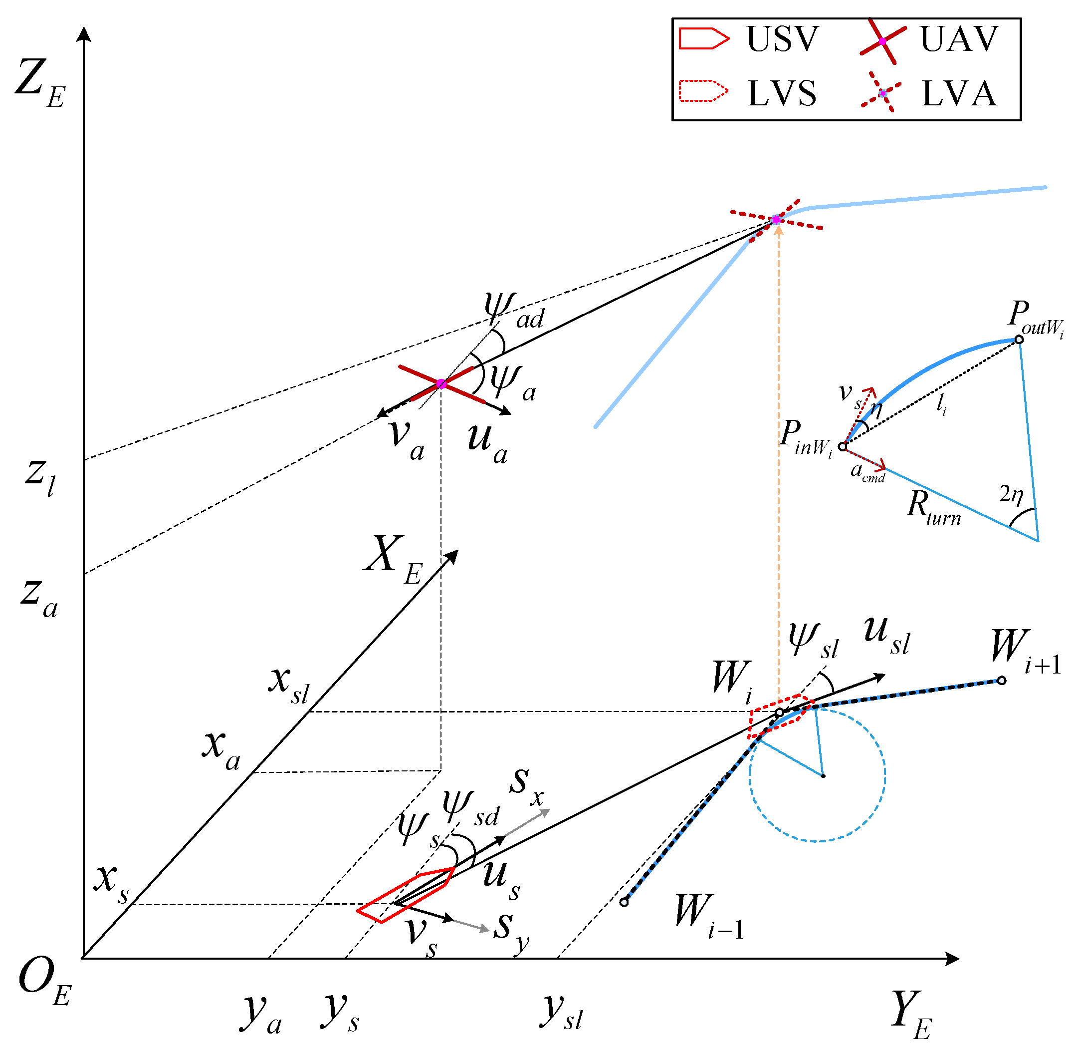
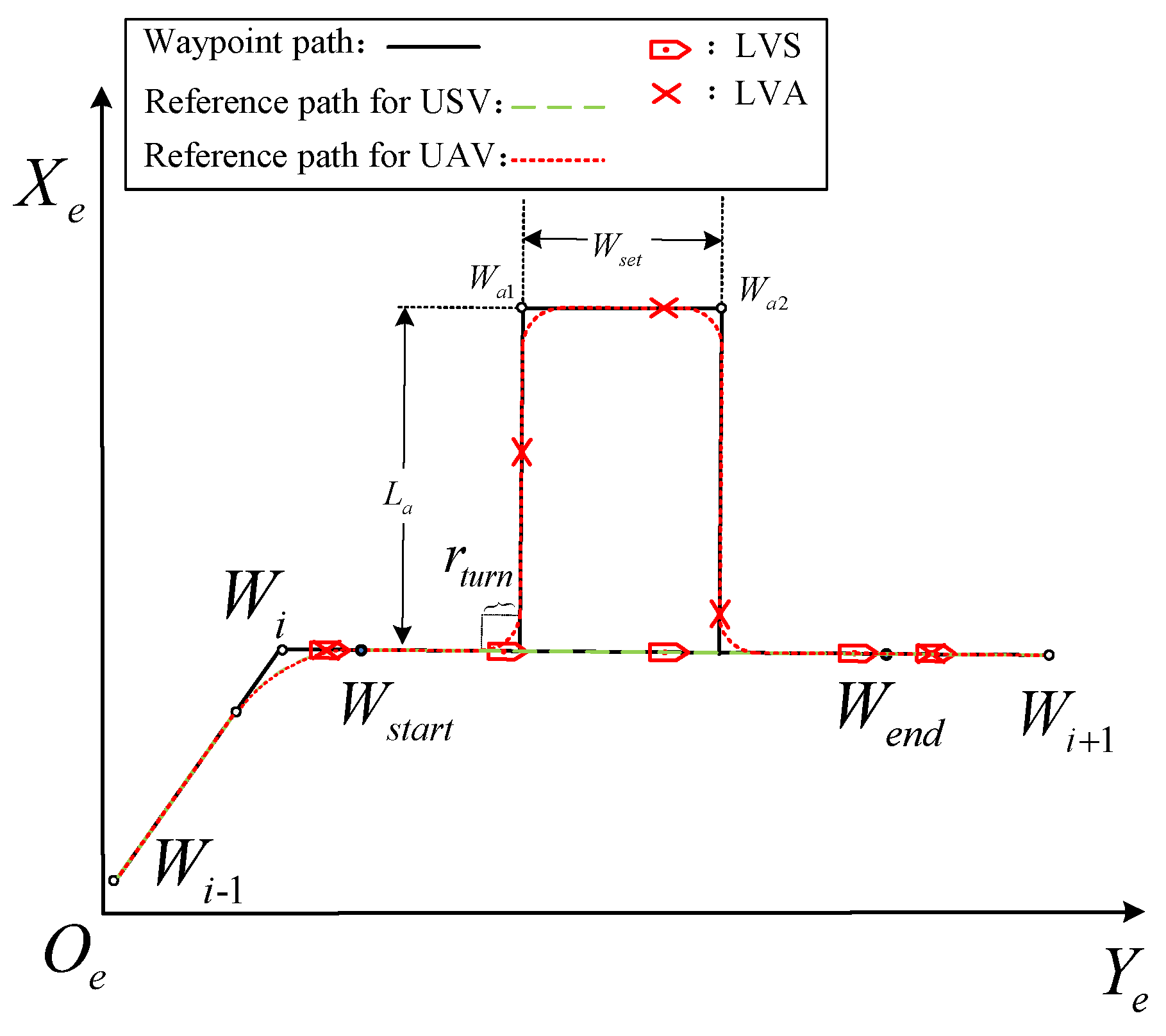
3. Asynchronous Separate Guidance Principle

To accomplish the multi-tasks carried out by the cooperative USV-UAV system, a novel asynchronous separate guidance principle was proposed. There are two tiers in the proposed guidance principle, one for USV (Section 3.1) and another for UAV (Section 3.2). In order to be more relevant to the actual, a new reference path was generated from pre-determined waypoints and this was based on velocity.

3.1. The Guidance Principle for USV

In [40], the guidance loop features an anticipatory control component that surmounts the intrinsic constraints of feedback control when tracking curved trajectories. Furthermore, although a similar path was planned in the curved sections, it was more relevant and practical to eliminate cumulative errors. Although [40] predominantly focused on UAVs, comparable concepts may be utilized in cooperative USV-UAV systems.

In Figure 2, the reference path is generated by the waypoints $W_1,W_2,\dots ,W_{i+1}$ with $W_i=\left(x_i,y_i\right)$. The waypoints-based reference path is made up of straight lines and curved lines [9]. Suppose the straight line between $W_i$ to $W_{i+1}$ is $L_{w_i}$. The guidance of straight lines is the same as the guidance in [12], and as in the guidance of curved lines, a similar path planning has been made. As shown in Figure 2, the curved line is a circular arc, $P_{in{W}_i}$ is a lateral acceleration command which has been generated using the reference point $W_i$. The reference point $P_{in{W}_i}$ is positioned on the intended trajectory at a distance ($l_i$) ahead of the $P_{out{W}_i}$. According to [40], the lateral acceleration command can be calculated by

$$a_{s_{cmd}}=2\frac{v_s^2}{l_i}\sin \eta$$

(11)

$\eta$ is the angle between the line $P_{in{W}_i}\to P_{out{W}_i}$ and the direction of the USV. Similarly, assume ${\eta }_a$ is the angle of the UAV, one has the lateral acceleration command of the UAV $a_{a_{cmd}}$ as

$$a_{a_{cmd}}=2\frac{v_a^2}{l_i}\sin {\eta }_a$$

(12)

The centripetal acceleration required to follow this instantaneous circular path is equal to the acceleration command produced by (11) and (12). Hence, the guidance principle will generate a lateral acceleration that is suitable for tracing a circular path with any radius R, which is a suitable alternative to the curve guidance in [8]. Respectively, one has the path information of the USV as

$$\left\{\begin{array}{c}{\dot{x}}_{sl}=u_{sl}\cos {\psi }_{sl}\hfill \\ {\dot{y}}_{sl}=u_{sl}\sin {\psi }_{sl}\hfill \\ {\dot{\psi }}_{sl}=r_{sl}\hfill \end{array}\right.$$

(13)

where $r_{sl}=a_{s_{cmd}}/u_{sl}$, which is the desired yaw angle velocity of the USV, $u_{sl}$ is the desired velocity, and $x_{sl},y_{sl},{\psi }_{sl}$ are the position and heading angles of the LVS. Therefore, the guidance law of the yaw degree can be expressed as ${\psi }_{sd}=\arctan \left[\left(y_{sl}-y_s\right)/\left(x_{sl}-x_s\right)\right]$ $+\left\{\left[1-\mathrm{sgn}(x_{sl}-x_s)\right]\mathrm{sgn}(y_{sl}-y_s)\pi \right\}/2$.

Remark 3.

Compare to the former guidance principle in [12], although the similar path planning has been made, the guidance for the virtual vessel in curved lines is different. The previous guidance principle is processed using a time-based calculation. The route planning in curved lines is planned after calculating the entire route. However, in marine practice, the total time cannot be determined once the waypoints are selected. Moreover, the proposed guidance principle is calculated based on the desired velocity and its distance to the target point, which is more relevant in practice. Furthermore, the proposed method also eliminates the cumulative error. Additionally, when compared to the path planning in [14], the curved lines are more relevant to marine practice.

3.2. The Guidance Principle for UAV

In order to accomplish cooperative multi-tasks between USV-UAV systems, and to take full advantage of the subsystems, a novel guidance principle aiming to complete the separation and rendezvous of the USV-UAV system was developed. As shown in Figure 3, when the USV-UAV system navigates to $W_{start}$, the UAV commences separation from the USV and begins to accelerate. $L_a$ is the distance of the desired path of the USV from the target area and $W_{set}$ is the length of the target area, which can be determined by the operator. When the UAV and the USV are approaching $W_{end}$, the UAV will decelerate once A and B have both decelerated to the same velocity. After passing $W_{end}$, the UAV will rendezvous with the USV. Thus, one has the path information of the UAV as

$$\left\{\begin{array}{c}{\dot{x}}_{al}=u_{al}\cos {\psi }_{al}\hfill \\ \begin{array}{l}{\dot{y}}_{al}=u_{al}\sin {\psi }_{al}\\ {\dot{z}}_{al}={\dot{z}}_{set}\end{array}\hfill \\ {\dot{\psi }}_{al}=r_{al}\hfill \end{array}\right.$$

(14)

where $r_{al}=a_{a_{cmd}}/u_{al}$, $u_{al}$ is the desired velocity of the UAV. $z_{set}$ is the desired height of the UAV, which is set by the user. As mentioned above, in order to guarantee the UAV can fly along with the USV when the multi-tasks are complete, the speed of the UAV should be specifically designated after separation. $u_{al}$ is related to $u_{sl}$. $u_{al}$ and ${\psi }_{ad}$ can be expressed as follows:

$$\left\{\begin{array}{l}{u}_{al} = \frac{2L_{ a }+L_{ w_i}+(2\pi -8)r_{turn}}{L_{ w_i }/u_{sl}}\hfill \\ {\psi }_{ad}=\arctan \left(\frac{y_{al}-y_a}{x_{al}-x_a}\right)+\frac{1}{2}\left[1-\mathrm{sgn}(x_{al}-x_a)\right]\mathrm{sgn}(y_{al}-y_a)\pi \hfill \end{array}\right.$$

(15)

Remark 4.

The main superiorities of the proposed asynchronous separate guidance principle can be concluded into two folds. Firstly, it can give full play to the advantages of the USV-UAV system: the strong mobility and broad vision of the UAV and the high endurance of the USV. Secondly, $L_a$ and $W_{set}$ can be determined by the user, which can be adapted for different situations.

4. Control Design

For reducing the transmission load, a fuzzy quantized controller based on the FLS is raised in this section. The control part can be divided into two steps, one is for the position loop (Section 4.1) and the other is for the attitude loop (Section 4.2). Then the Proof of stability is shown in Section 4.3. The main control framework of the USV-UAV system can be seen as Figure 4.

4.1. Control Design for the Position Loop

Step 1: At this step, the position error for USV-UAV systems can be introduced as follows.

$$\left\{\begin{array}{c}{x}_{ie}=x_i-x_{il}\\ y_{ie}=y_i-y_{il}\\ z_{ae}=z_a-z_{set}\end{array}\right.$$

(16)

where $i=s,a$, one assumes $z_{se}=\sqrt{x_{se}^2+y_{se}^2}$ to simplify the subsequent control design. $z_{set}$ is predetermined by the user according to the actual situation. The derivatives of position error can be expressed as

$$\left\{\begin{array}{l}{\dot{z}}_{se}=\varpi -u_{au}\cos {\psi }_{se}\hfill \\ {\dot{x}}_{ae}={\dot{x}}_a-{\dot{x}}_{al}\hfill \\ {\dot{y}}_{ae}={\dot{y}}_a-{\dot{y}}_{al}\hfill \\ {\dot{z}}_{ae}={\dot{z}}_a-{\dot{z}}_{set}\hfill \end{array}\right.$$

(17)

where ${\psi }_{se}={\psi }_s-{\psi }_{sl},\varpi ={\dot{x}}_{sl}\cos \left({\psi }_{sl}\right)+{\dot{y}}_{sl}\sin \left({\psi }_{sl}\right)-v_s\sin \left({\psi }_{sl}\right)$.${\psi }_{se}$ is the attitude error of the USV. Respectively, ${\psi }_s,{\psi }_{sl}$ are the intended heading angle and virtual heading angle of the USV. Referring to the following errors, the virtual control law can be chosen as (18).

$$\left\{\begin{array}{l}{\alpha }_{ue}=\cos {({\psi }_{se})}^{-1}[k_{ue}(z_{se}-\delta )+\varpi ]\hfill \\ {\alpha }_{xe}=-k_{xe}{x}_{ae}+\stackrel{.}{x_{al}}\hfill \\ {\alpha }_{ye}=-k_{ye}{y}_{ae}+\stackrel{.}{y_{al}}\hfill \\ {\alpha }_{ze}=-k_{ze}{z}_{ae}+\stackrel{.}{z_{set}}\hfill \end{array}\right.$$

(18)

where ${\alpha }_{\varsigma e}$ is the virtual control, $k_{\varsigma e},\varsigma =u,x,y,z$ is the positive control parameter, and $\delta$ is a tiny quantity to ensure the LVS is in front of the USV. In order to avoid the high computational cost, which is called “explosion of complexity”, the DSC technique will be introduced next.

$${\beta }_{\varsigma }=\frac{{\alpha }_{\varsigma }}{1+{ϵ}_{\varsigma }s},{\beta }_{\varsigma }\left(0\right)={\alpha }_{\varsigma }\left(0\right)$$

(19)

where ${\beta }_{\varsigma }$ is first-order filter, ${ϵ}_{\varsigma }$ is time constant and $s$ is the Laplace operator. One defines the DSC error $q_{\varsigma }={\beta }_{\varsigma }-{\alpha }_{\varsigma },\varsigma =u,x,y,z$. Then the derivative of $q_{\varsigma }$ can be described as (20).

$$\stackrel{.}{q_{\varsigma }}={\dot{\beta }}_{\varsigma }-{\dot{\alpha }}_{\varsigma }=-\frac{q_{\varsigma }}{{ϵ}_{\varsigma }}+B_{\varsigma }(\cdot )$$

(20)

where $B_{\varsigma }(\cdot )$ is the continuous bounded function with upper bound $M_{\varsigma }$.

Step 2. Define the error $u_{\varsigma e}=u_{a\varsigma }-{\beta }_{\varsigma e},\varsigma =u,x,y,z$, hence the derivation of $u_{\varsigma e}$ can be described as

$$\left\{\begin{array}{c}\stackrel{.}{u_{ue}}=-\stackrel{.}{{\beta }_u}+\frac{1}{m_u}\left[f_u(u)+{\tau }_u\right]+d_{wu}+{\epsilon }_u\hfill \\ \stackrel{.}{u_{xe}}=-\stackrel{.}{{\beta }_x}+f_x(x)+\frac{1}{m}{R}_x{F}_f+d_{wx}+{\epsilon }_x\hfill \\ \stackrel{.}{u_{ye}}=-\stackrel{.}{{\beta }_y}+f_y(y)+\frac{1}{m}{R}_y{F}_f+d_{wy}+{\epsilon }_y\hfill \\ \stackrel{.}{u_{ze}}=-\stackrel{.}{{\beta }_z}+f_z(z)+\frac{1}{m}{R}_z{F}_f+d_{wz}+{\epsilon }_z\hfill \end{array}\right.$$

(21)

where the unknown nonlinear function $f_{\varsigma }\left(\cdot \right)$, $\varsigma =u,x,y,s$ can be approximated by FLS as

$$f_{\varsigma }\left(\varsigma \right)={\mathit{\omega }}_{\varsigma }^T{\mathit{\phi }}_{\varsigma }\left(\varsigma \right)+{\epsilon }_{\varsigma }$$

(22)

$f_{\varsigma }\left(\cdot \right)$ is an unknown smooth function which can be approximated by FLS. Define $\varsigma i=x,y,z$, one has

$$\begin{array}{cc}\hfill -\frac{m_v}{m_u}vr+{\mathit{\omega }}_u^T{\mathit{\phi }}_u\left(u\right)+{\epsilon }_u& \le \frac{m_v}{m_u}\left(\frac{v^2+r^2}{2}\right)+{‖{\mathit{\omega }}_u^T{\mathit{\phi }}_u\left(u\right)+{\epsilon }_u‖}_2\hfill \\ \hfill & \le \max \left\{\frac{m_v}{m_u},{‖{\mathit{\omega }}_{\varsigma }^T‖}_2,{\overline{\epsilon }}_u\right\}\left(\frac{v^2+r^2}{2}+{‖{\mathit{\phi }}_{\varsigma }\left(\varsigma \right)‖}_2+1\right)\hfill \\ \hfill & \le \frac{1}{m_u}{\vartheta }_u{\gamma }_u\hfill \end{array}$$

(23)

$$\begin{array}{cc}\hfill {\mathit{\omega }}_{\varsigma i}^T{\mathit{\phi }}_{\varsigma i}\left(\varsigma i\right)+{\epsilon }_{\varsigma i}& \le {‖{\mathit{\omega }}_{\varsigma i}^T{\mathit{\phi }}_{\varsigma i}\left(\varsigma i\right)+{\epsilon }_{\varsigma i}‖}_2\hfill \\ \hfill & \le \max \left\{{‖{\mathit{\omega }}_{\varsigma i}^T‖}_2,{\overline{\epsilon }}_{\varsigma i}\right\}\left({‖{\mathit{\phi }}_{\varsigma i}\left(\varsigma i\right)‖}_2+1\right)\hfill \\ \hfill & \le {\vartheta }_{\varsigma i}{\gamma }_{\varsigma i}\hfill \end{array}$$

(24)

where ${\vartheta }_u=m_u\max \left\{m_v/m_u,{‖{\mathit{\phi }}_u^T‖}_2,{\overline{\epsilon }}_u\right\}$, ${\vartheta }_{\varsigma i}=\max \left\{{‖{\mathit{\phi }}_{\varsigma i}^T‖}_2,{\overline{\epsilon }}_{\varsigma i}\right\}$ refer to the unknown parameters. As for ${\gamma }_{\varsigma i}$ and ${\gamma }_u$, they are the damping term which can be calculated as ${\gamma }_u=\left(v^2+r^2\right)/2+{‖{\mathit{\omega }}_u\left(u\right)‖}_2+1$, ${\gamma }_{\varsigma i}={‖{\mathit{\omega }}_{\varsigma i}\left(\varsigma i\right)‖}_2+1$. Based on the above analysis, the derivation of the $u_{\varsigma e}$ can be rewritten as

$$\left\{\begin{array}{l}{\dot{u}}_{ue}=-{\dot{\beta }}_u+\frac{1}{m_u}{\vartheta }_u{\gamma }_u+\frac{{\tau }_u}{m_u}+d_{wu}\hfill \\ \stackrel{.}{u_{xe}}=-\stackrel{.}{{\beta }_x}+{\vartheta }_x{\gamma }_x+\frac{1}{m}{R}_x{F}_f+d_{wx}+{\epsilon }_x\hfill \\ \stackrel{.}{u_{ye}}=-\stackrel{.}{{\beta }_y}+{\vartheta }_y{\gamma }_y+\frac{1}{m}{R}_y{F}_f+d_{wy}+{\epsilon }_y\hfill \\ \stackrel{.}{u_{ze}}=-\stackrel{.}{{\beta }_z}+{\vartheta }_z{\gamma }_z+\frac{1}{m}{R}_z{F}_f+d_{wz}+{\epsilon }_z\hfill \end{array}\right.$$

(25)

To simplify the control design, the intermediate variables designed as the control inputs of the position loop of the USV-UAV system can be listed as follows:

$$\left\{\begin{array}{l}{\mathrm{\Gamma }}_u\cdot {\chi }_{ue}=\frac{{\tau }_u}{m_u}\hfill \\ {\mathrm{\Gamma }}_x\cdot {\chi }_{xe}=\frac{1}{m}{R}_x{F}_f\hfill \\ {\mathrm{\Gamma }}_y\cdot {\chi }_{ye}=\frac{1}{m}{R}_y{F}_f\hfill \\ {\mathrm{\Gamma }}_z\cdot {\chi }_{ze}=-g+\frac{1}{m}{R}_z{F}_f\hfill \end{array}\right.$$

(26)

${\mathrm{\Gamma }}_{\varsigma }$ is the corresponding adaptive law, defined as ${\xi }_{\varsigma }=1/{\mathrm{\Gamma }}_{\varsigma },\varsigma =u,x,y,z$. Furthermore, one has the position control law (27) and the corresponding adaptive law (28)

$$\left\{\begin{array}{l}{\chi }_{ue}=-k_u{u}_{ue}+\stackrel{.}{{\beta }_u} - {\widehat{\lambda }}_u{\kappa }_u{u}_{ue}\hfill \\ {\chi }_{xe}=-k_x{u}_{xe}+\stackrel{.}{{\beta }_x} -{\widehat{\lambda }}_x{\kappa }_x{u}_{xe} -x_{ae}\hfill \\ {\chi }_{ye}=-k_y{u}_{ye}+\stackrel{.}{{\beta }_y}-{\widehat{\lambda }}_y{\kappa }_y{u}_{ye} -y_{ae}\hfill \\ {\chi }_{ze}=-k_z{u}_{ze}+\stackrel{.}{{\beta }_z}-{\widehat{\lambda }}_z{\kappa }_z{u}_{ze} -z_{ae}\hfill \end{array}\right.$$

(27)

$$\left\{\begin{array}{c}{\dot{\widehat{\lambda }}}_{\varsigma }=k_{\lambda \varsigma }^{-1}\cdot [{\mu }_{\lambda \varsigma }{u}_{\varsigma e}^{}-k_{\lambda }^{\varsigma }({\widehat{\lambda }}_{\varsigma }-{\widehat{\lambda }}_{\varsigma }(0))]\\ {\dot{\widehat{\mathrm{\Gamma }}}}_{\varsigma }=k_{\mathrm{\Gamma }\varsigma }^{-1}\cdot [{\chi }_{\varsigma e}{u}_{\varsigma e}^{}-k_{\mathrm{\Gamma }}^{\varsigma }({\widehat{\mathrm{\Gamma }}}_{\varsigma }-{\widehat{\mathrm{\Gamma }}}_{\varsigma }(0))]\end{array}\right.$$

(28)

where $k_{\lambda \varsigma },k_{\mathrm{\Gamma }\varsigma },k_{\lambda }^{\varsigma },k_{\mathrm{\Gamma }}^{\varsigma }$, $\varsigma =u,x,y,z$ are positive control parameters, ${\widehat{\lambda }}_{\varsigma },{\widehat{\mathrm{\Gamma }}}_{\varsigma }$ are the estimations of ${\lambda }_{\varsigma },{\mathrm{\Gamma }}_{\varsigma }$. ${\widehat{\lambda }}_{\varsigma }(0),{\widehat{\mathrm{\Gamma }}}_{\varsigma }(0)$ denote the initial value of ${\widehat{\lambda }}_{\varsigma },{\widehat{\mathrm{\Gamma }}}_{\varsigma }$. ${\lambda }_{\varsigma }$ refers to the larger of ${\vartheta }_u$ or $‖{\mathit{\omega }}_{\varsigma }^T‖$. ${\mu }_{\lambda \varsigma }$ can be calculated based on the weight of the FLS.

4.2. Control Design for the Attitude Loop

The reference heading angles of the UAV can be expressed as

$$\begin{array}{l}{\varphi }_{al}=\arctan \left(\cos ({\theta }_{al})\frac{\sin ({\psi }_{al}){\chi }_{xe}-\cos ({\psi }_{al}){\chi }_{ye}}{{\chi }_{ze}+g}\right)\\ {\theta }_{al}=\arctan \left(\frac{\cos ({\psi }_{al}){\chi }_{xe}-\sin ({\psi }_{al}){\chi }_{ye}}{{\chi }_{ze}+g}\right)\end{array}$$

(29)

Step 1: At this step, the attitude error for the USV-UAV system can be designed as follows:

$$\left\{\begin{array}{l}{\psi }_{se}={\psi }_s-{\psi }_{sd}\\ {\psi }_{ae}={\psi }_a-{\psi }_{ad}\\ {\varphi }_{ae}={\varphi }_a-{\varphi }_{al}\\ {\theta }_{ae}={\theta }_a-{\theta }_{al}\end{array}\right.$$

(30)

Notably, the UAV may move from the back of the LVS to the front in a short period of time as the speed of the UAV is significant and easily affected by external conditions. The attitude error may vary between -pi and pi when there is considerable external interference, however, the actual error is not of great magnitude. One can obtain the derivative of (30) as

$$\left\{\begin{array}{l}\stackrel{.}{{\psi }_{se}}=r_{ar}-\stackrel{.}{{\psi }_{sd}}\hfill \\ \stackrel{.}{{\psi }_{ae}}=r_{a\psi }-\stackrel{.}{{\psi }_{ad}}\hfill \\ \stackrel{.}{{\varphi }_{ae}}=r_{a\varphi }-\stackrel{.}{{\varphi }_{ad}}\hfill \\ \stackrel{.}{{\theta }_{ae}}=r_{a\theta }-\stackrel{.}{{\theta }_{ad}}\hfill \end{array}\right.$$

(31)

Similar to (18), one has the virtual controls laws for the attitude loop as

$$\left\{\begin{array}{l}{\alpha }_{re}=-k_{re}{\psi }_{se}+\stackrel{.}{{\psi }_{sd}}\hfill \\ {\alpha }_{\psi e}=-k_{\psi e}{\psi }_{ae}+\stackrel{.}{{\psi }_{al}}\hfill \\ {\alpha }_{\varphi e}=-k_{\varphi e}{\varphi }_{ae}+\stackrel{.}{{\varphi }_{ad}}\hfill \\ {\alpha }_{\theta e}=-k_{\theta e}{\theta }_{ae}+\stackrel{.}{{\theta }_{ad}}\hfill \end{array}\right.$$

(32)

where $k_{re},k_{\psi e},k_{\varphi e},k_{\theta e}$ are positive control parameters. Similarly, the DSC technique is also applied in the attitude loop.

$${\beta }_{\sigma }=\frac{{\alpha }_{\sigma }}{1+{ϵ}_{\sigma }s},{\beta }_{\sigma }\left(0\right)={\alpha }_{\sigma }\left(0\right)$$

(33)

where ${\beta }_{\sigma }$ is first-order filter, ${ϵ}_{\sigma }$ is time constant, and $s$ is the Laplace operator. One defines the DSC error $q_{\sigma }={\beta }_{\sigma }-{\alpha }_{\sigma },\sigma =r,\psi ,\varphi ,\theta$. Then the derivative of $q_{\sigma }$ can be described as (34).

$$\stackrel{.}{q_{\sigma }}={\dot{\beta }}_{\sigma }-{\dot{\alpha }}_{\sigma }=-\frac{q_{\sigma }}{{ϵ}_{\sigma }}+B_{\sigma }(\cdot )$$

(34)

where $B_{\sigma }(\cdot )$ is the continuous bounded function with upper bound $M_{\sigma }$.

Step 2. Define the error $r_{\sigma e}=r_{a\sigma }-{\beta }_{\sigma e}$, $\sigma =r,\psi ,\varphi ,\theta$, hence the derivation of the $r_{\sigma e}$ can be obtained.

$$\left\{\begin{array}{l}\stackrel{.}{r_{re}}=-\stackrel{.}{{\beta }_r}+\frac{1}{m_r}\left[f_r(r)+{\tau }_r\right]+d_{wr}+{\epsilon }_r\hfill \\ \stackrel{.}{r_{\psi e}}=-\stackrel{.}{{\beta }_{\psi }}+f_{\psi }(\psi )+\frac{d}{I_{zz}}{\tau }_{\psi }+d_{w\psi }+{\epsilon }_{\psi }\hfill \\ \stackrel{.}{r_{\varphi e}}=-\stackrel{.}{{\beta }_{\varphi }}+f_{\varphi }(\varphi )+\frac{d}{I_{xx}}{\tau }_{\varphi }+d_{w\varphi }+{\epsilon }_{\varphi }\hfill \\ \stackrel{.}{r_{\theta e}}=-\stackrel{.}{{\beta }_{\theta }}+f_{\theta }(\theta )+\frac{d}{I_{yy}}{\tau }_{\theta }+d_{w\theta }+{\epsilon }_{\theta }\hfill \end{array}\right.$$

(35)

where the unknown nonlinear functions $f_{\sigma }\left(\cdot \right)$, $\sigma =r,\psi ,\varphi ,\theta$ can be approximated by FLS as

$$f_{\sigma }\left(\sigma \right)={\mathit{\omega }}_{\sigma }^T{\mathit{\phi }}_{\sigma }\left(\sigma \right)+{\epsilon }_{\sigma }$$

(36)

$f_{\sigma }\left(\cdot \right)$ is an unknown smooth function which can be approximated by FLS. To define $\sigma i=\psi ,\varphi ,\theta$, one has

$$-\frac{m_u-m_v}{m_r}vu+{\mathit{\omega }}_r^T{\mathit{\phi }}_r\left(r\right)+{\epsilon }_r\le \frac{1}{m_r}{\vartheta }_r{\gamma }_r$$

(37)

$${\mathit{\omega }}_{\sigma i}^T{\mathit{\phi }}_{\sigma i}\left(\sigma i\right)+{\epsilon }_{\sigma i}\le {\vartheta }_{\sigma i}{\gamma }_{\sigma i}$$

(38)

where ${\vartheta }_r=m_r\max \left\{m_u-m_v/m_r,{‖{\mathit{\phi }}_r^T‖}_2,{\overline{\epsilon }}_r\right\},{\vartheta }_{\sigma i}=\max \left\{{‖{\mathit{\phi }}_{\sigma i}^T‖}_2,{\overline{\epsilon }}_{\sigma i}\right\}$ refers to the unknown parameters. As for ${\gamma }_r,{\gamma }_{\sigma i}$, they are the damping term which can be calculated as ${\gamma }_r=\left(v^2+u^2\right)/2+{‖{\mathit{\omega }}_r\left(r\right)‖}_2+1$, ${\gamma }_{\sigma i}={‖{\mathit{\omega }}_{\sigma i}\left(\sigma i\right)‖}_2+1$. Based on the above analysis, the derivation of the $r_{\sigma e}$ can be rewritten as

$$\left\{\begin{array}{c}\stackrel{.}{r_{re}}=-\stackrel{.}{{\beta }_r}+\frac{1}{m_r}\left[{\vartheta }_r{\gamma }_r+{\tau }_r\right]+d_{wr}+{\epsilon }_r\\ \stackrel{.}{r_{\psi e}}=-\stackrel{.}{{\beta }_{\psi }}+{\vartheta }_{\psi }{\gamma }_{\psi }+\frac{d}{I_{zz}}{\tau }_{\psi }+d_{w\psi }+{\epsilon }_{\psi }\\ \stackrel{.}{r_{\varphi e}}=-\stackrel{.}{{\beta }_{\varphi }}+{\vartheta }_{\varphi }{\gamma }_{\varphi }+\frac{d}{I_{xx}}{\tau }_{\varphi }+d_{w\varphi }+{\epsilon }_{\varphi }\\ \stackrel{.}{r_{\theta e}}=-\stackrel{.}{{\beta }_{\theta }}+{\vartheta }_{\theta }{\gamma }_{\theta }+\frac{d}{I_{yy}}{\tau }_{\theta }+d_{w\theta }+{\epsilon }_{\theta }\end{array}\right.$$

(39)

In order to simplify the control design, the intermediate variables, which are designed as the control input of the attitude loop of the USV-UAV system, are shown as

$$\left\{\begin{array}{l}{\mathrm{\Gamma }}_r\cdot {\chi }_{re}=\frac{{\tau }_r}{m_r}\hfill \\ {\mathrm{\Gamma }}_{\psi }\cdot {\chi }_{\psi e}=\frac{d}{I_{zz}}{\tau }_{\psi }\hfill \\ {\mathrm{\Gamma }}_{\varphi }\cdot {\chi }_{\varphi e}=\frac{d}{I_{yy}}{\tau }_{\varphi }\hfill \\ {\mathrm{\Gamma }}_{\theta }\cdot {\chi }_{\theta e}=\frac{d}{I_{xx}}{\tau }_{\theta }\hfill \end{array}\right.$$

(40)

${\mathrm{\Gamma }}_{\sigma }$ is the corresponding adaptive law, which is defined as ${\xi }_{\sigma }=1/{\mathrm{\Gamma }}_{\sigma },\sigma =r,\psi ,\varphi ,\theta$. Furthermore, one has the control law and the corresponding adaptive law as follows:

$$\left\{\begin{array}{l}{\chi }_{re}=-k_r{r}_{re}+\stackrel{.}{{\beta }_r} - {\widehat{\lambda }}_r{\kappa }_r{r}_{re}\hfill \\ {\chi }_{\psi e}=-k_{\psi }{r}_{\psi e}+\stackrel{.}{{\beta }_{\psi }} -{\widehat{\lambda }}_{\psi }{\kappa }_{\psi }{r}_{\psi e} -{\psi }_{ae}\hfill \\ {\chi }_{\varphi e}=-k_{\varphi }{r}_{\varphi e}+\stackrel{.}{{\beta }_{\varphi }}-{\widehat{\lambda }}_{\varphi }{\kappa }_{\varphi }{r}_{\varphi e} -{\varphi }_{ae}\hfill \\ {\chi }_{\theta e}=-k_{\theta }{r}_{\theta e}+\stackrel{.}{{\beta }_{\theta }}-{\widehat{\lambda }}_{\theta }{\kappa }_{\theta }{r}_{\theta e} -{\theta }_{ae}\hfill \end{array}\right.$$

(41)

$$\left\{\begin{array}{c}{\dot{\widehat{\lambda }}}_{\sigma }=k_{\lambda \sigma }^{-1}\cdot [{\mu }_{\lambda \sigma }{r}_{\sigma e}^{}-k_{\lambda }^{\sigma }({\widehat{\lambda }}_{\sigma }(t)-{\widehat{\lambda }}_{\sigma }(0))]\\ {\dot{\widehat{\mathrm{\Gamma }}}}_{\sigma }=k_{\mathrm{\Gamma }\sigma }^{-1}\cdot [{\chi }_{\sigma e}{r}_{\sigma e}^{}-k_{\mathrm{\Gamma }}^{\sigma }({\widehat{\mathrm{\Gamma }}}_{\sigma }-{\widehat{\mathrm{\Gamma }}}_{\sigma }(0))]\end{array}\right.$$

(42)

where $k_{\lambda \sigma },k_{\mathrm{\Gamma }\sigma },k_{\lambda }^{\sigma },k_{\mathrm{\Gamma }}^{\sigma }$ in which $\sigma =r,\psi ,\varphi ,\theta$ are positive control parameters, ${\widehat{\lambda }}_{\sigma },{\widehat{\mathrm{\Gamma }}}_{\sigma }$ are the respective estimations of ${\lambda }_{\sigma },{\mathrm{\Gamma }}_{\sigma }$. ${\widehat{\lambda }}_{\sigma }(0),{\widehat{\mathrm{\Gamma }}}_{\sigma }(0)$ denote the initial values of ${\widehat{\lambda }}_{\sigma },{\widehat{\mathrm{\Gamma }}}_{\sigma }$. ${\lambda }_{\sigma }$ refers to the larger of the ${\vartheta }_{\sigma }$ or $‖{\mathit{\omega }}_{\sigma }^T‖$. ${\mu }_{\lambda \sigma }$ can be calculated based on the weight of the FLS.

Remark 5.

During the course of the USV-UAV system, its velocity must be adjusted in real-time to accommodate intricate external conditions, despite infrequent alterations in its heading. The utilization of a hysteresis quantizer enables the input heading signal to fluctuate at a low frequency around a specific value, which unquestionably meets the requirements of the system whilst reducing the number of actuator executions and wear and tear between sensors.

4.3. Stability Analysis

In this section, the stability analysis has been carried out to prove that all the error variables in the USV-UAV systems are semi-globally uniform ultimate bounded (SGUUB) on the basis of the control design process in Section 4.1 and Section 4.2, and the main result can be summarized as Theorem 1.

Theorem 1.

Considering the closed-loop USV-UAV system with the assumptions 1–4, the control law and the adaptive law. For all initial conditions satisfying ${(z_{se}^{}-\delta )}^2\left(0\right)$$+$$x_{ae}^2\left(0\right)$$+$$y_{ae}^2\left(0\right)$$+$$z_{ae}^2\left(0\right)$$+$${\displaystyle \sum _{\varsigma =u,x,y,z}\left[q_{\varsigma }^2\left(0\right)+u_{\varsigma e}^2\left(0\right)+k_{\lambda \varsigma }^{}{\dot{\tilde{\lambda }}}_{\varsigma }^2\left(0\right)+k_{\mathrm{\Gamma }\varsigma }^{}{\xi }_{\varsigma }{\dot{\tilde{\mathrm{\Gamma }}}}_{\varsigma }^2\left(0\right)\right]}$$+$${\psi }_{se}^2\left(0\right)$$+$${\psi }_{ae}^2\left(0\right)$$+$${\varphi }_{ae}^2\left(0\right)$$+$${\theta }_{ae}^2\left(0\right)$$+$${\displaystyle \sum _{\sigma =r,\psi ,\varphi ,\theta }\left[q_{\sigma }^2\left(0\right)+r_{\sigma e}^2\left(0\right)+k_{\lambda \sigma }^{}{\dot{\tilde{\lambda }}}_{\sigma }^2\left(0\right)+k_{\mathrm{\Gamma }\sigma }^{}{\xi }_{\sigma }{\dot{\tilde{\mathrm{\Gamma }}}}_{\sigma }^2\left(0\right)\right]}$$\le$$2\mathrm{\Delta }$ with any $\mathrm{\Delta }>0$, all the signals in the closed-loop system are SGUUB by choosing the appropriate design parameters.

Proof. 

Constructing the following Lyapunov function candidate:

$$\begin{array}{c}V=\frac{1}{2}{(z_{se}^{}-\delta )}^2+\frac{1}{2}{x}_{ae}^2+\frac{1}{2}{y}_{ae}^2+\frac{1}{2}{z}_{ae}^2+\frac{1}{2}{\displaystyle \sum _{\varsigma =u,x,y,z}\left[q_{\varsigma }^2+u_{\varsigma e}^2+k_{\lambda \varsigma }^{}{\tilde{\lambda }}_{\varsigma }^2\left.+k_{\mathrm{\Gamma }\varsigma }^{}{\xi }_{\varsigma }{\tilde{\mathrm{\Gamma }}}_{\varsigma }^2\right]\right.}\\ +\frac{1}{2}{\psi }_{se}^2+\frac{1}{2}{\psi }_{ae}^2+\frac{1}{2}{\varphi }_{ae}^2+\frac{1}{2}{\theta }_{ae}^2+\frac{1}{2}{\displaystyle \sum _{\sigma =r,\psi ,\varphi ,\theta }\left[q_{\sigma }^2+r_{\sigma e}^2+k_{\lambda \sigma }^{}{\tilde{\lambda }}_{\sigma }^2\left.+k_{\mathrm{\Gamma }\sigma }^{}{\xi }_{\sigma }{\tilde{\mathrm{\Gamma }}}_{\sigma }^2\right]\right.}\end{array}$$

(43)

Thus, the time derivative of $V$ can be expressed as

$$\begin{array}{cc}\hfill \dot{V}& =(z_{se}^{}-\delta ){\dot{z}}_{se}^{}+x_{ae}^{}{\dot{x}}_{ae}^{}+y_{ae}^{}{\dot{y}}_{ae}^{}+z_{ae}^{}{\dot{z}}_{ae}^{}+{\displaystyle \sum _{\varsigma =u,x,y,z}\left[q_{\varsigma }^{}{\dot{q}}_{\varsigma }^{}+u_{\varsigma e}^{}{\dot{u}}_{\varsigma e}^{}+k_{\lambda \varsigma }^{}{\tilde{\lambda }}_{\varsigma }^{}{\dot{\tilde{\lambda }}}_{\varsigma }^{}\right.}\hfill \\ & \left.+k_{\mathrm{\Gamma }\varsigma }^{}{\xi }_{\varsigma }{\tilde{\mathrm{\Gamma }}}_{\varsigma }^2{\dot{\tilde{\mathrm{\Gamma }}}}_{\varsigma }^2\right]+{\psi }_{se}^{}{\dot{\psi }}_{se}^{}+{\psi }_{ae}^{}{\dot{\psi }}_{ae}^{}+{\varphi }_{ae}^{}{\dot{\varphi }}_{ae}^{}+{\theta }_{ae}^{}{\dot{\theta }}_{ae}^{}+{\displaystyle \sum _{\sigma =r,\psi ,\varphi ,\theta }\left[q_{\sigma }^{}{\dot{q}}_{\sigma }^{}+r_{\sigma e}^{}{\dot{r}}_{\sigma e}^{}\right.}\hfill \\ & +k_{\lambda \sigma }^{}{\tilde{\lambda }}_{\sigma }^{}{\dot{\tilde{\lambda }}}_{\sigma }^{}\left.+k_{\mathrm{\Gamma }\sigma }^{}{\xi }_{\sigma }{\tilde{\mathrm{\Gamma }}}_{\sigma }^{}{\dot{\tilde{\mathrm{\Gamma }}}}_{\sigma }^{}\right]\hfill \end{array}$$

(44)

Moreover, ${\lambda }_{\varsigma }{\dot{\lambda }}_{\varsigma }$ and ${\lambda }_{\sigma }{\dot{\lambda }}_{\sigma }$ can be devised as

$$\begin{array}{cc}{\lambda }_{\varsigma }{\dot{\lambda }}_{\varsigma }& =k_{\lambda \varsigma }^{-1}{\tilde{\lambda }}_{\varsigma }{\dot{\widehat{\lambda }}}_{\varsigma }\hfill \\ & =-k_{\lambda \varsigma }^{-1}\left[{\tilde{\lambda }}_{\varsigma }{\kappa }_{\varsigma }{u}_{\varsigma e}^2-k_{\lambda }^{\varsigma }{\tilde{\lambda }}_{\varsigma }\left({\lambda }_{\varsigma }+{\tilde{\lambda }}_{\varsigma }-{\widehat{\lambda }}_{\varsigma }\left(0\right)\right)\right]\hfill \\ & \le -k_{\lambda \varsigma }^{-1}\left[{\tilde{\lambda }}_{\varsigma }{\kappa }_{\varsigma }{u}_{\varsigma e}^2-\frac{k_{\lambda }^{\varsigma }{\tilde{\lambda }}_{\varsigma }^2}{2}+\frac{k_{\lambda }^{\varsigma }{\left({\lambda }_{\varsigma }-{\widehat{\lambda }}_{\varsigma }\left(0\right)\right)}^2}{2}\right]\hfill \end{array}$$

(45)

$${\lambda }_{\sigma }{\dot{\lambda }}_{\sigma }\le -k_{\lambda \sigma }^{-1}\left[{\tilde{\lambda }}_{\sigma }{\kappa }_{\sigma }{r}_{\sigma e}-\frac{k_{\lambda }^{\sigma }{\tilde{\lambda }}_{\sigma }^2}{2}+\frac{k_{\lambda }^{\sigma }{\left({\lambda }_{\sigma }-{\widehat{\lambda }}_{\sigma }\left(0\right)\right)}^2}{2}\right]$$

(46)

Similarly, ${\mathrm{\Gamma }}_{\varsigma }{\dot{\mathrm{\Gamma }}}_{\varsigma }$ and ${\mathrm{\Gamma }}_{\sigma }{\dot{\mathrm{\Gamma }}}_{\sigma }$ can be written as

$${\mathrm{\Gamma }}_{\varsigma }{\dot{\mathrm{\Gamma }}}_{\varsigma }\le -k_{\mathrm{\Gamma }\varsigma }^{-1}\left[{\tilde{\mathrm{\Gamma }}}_{\varsigma }{\chi }_{\varsigma }{u}_{\varsigma e}^2-\frac{k_{\mathrm{\Gamma }}^{\varsigma }{\tilde{\mathrm{\Gamma }}}_{\varsigma }^2}{2}+\frac{k_{\mathrm{\Gamma }}^{\varsigma }{\left({\mathrm{\Gamma }}_{\varsigma }-{\widehat{\mathrm{\Gamma }}}_{\varsigma }\left(0\right)\right)}^2}{2}\right]$$

(47)

$${\mathrm{\Gamma }}_{\sigma }{\dot{\mathrm{\Gamma }}}_{\sigma }\le -k_{\mathrm{\Gamma }\sigma }^{-1}\left[{\tilde{\mathrm{\Gamma }}}_{\sigma }{\chi }_{\sigma }{r}_{\sigma e}^2-\frac{k_{\mathrm{\Gamma }}^{\sigma }{\tilde{\mathrm{\Gamma }}}_{\sigma }^2}{2}+\frac{k_{\mathrm{\Gamma }}^{\sigma }{\left({\mathrm{\Gamma }}_{\sigma }-{\widehat{\mathrm{\Gamma }}}_{\sigma }\left(0\right)\right)}^2}{2}\right]$$

(48)

In addition, the following equations are useful for the stability analysis:

$$(z_{se}-\delta ){\dot{z}}_{se}\le -\left(k_{ue} -\frac{1}{2}\right){\left(z_{se}-\delta \right)}^2 +u_{ue}^2+q_u^2$$

(49)

$${\psi }_{se}{\dot{\psi }}_{se}\le -\left(k_{re}-\frac{1}{2}\right){\psi }_{se}^2+r_{re}^2+q_r^2$$

(50)

$$q_{\varsigma }{\dot{q}}_{\varsigma }\le q_{\varsigma }\left(M_{\varsigma }-\frac{q_{\varsigma }}{{ϵ}_{\varsigma }}\right)\le -\left(\frac{1}{{ϵ}_{\varsigma }}-\frac{M_{\varsigma }^2}{2a_{\varsigma }}\right)q_{\varsigma }^2+\frac{a_{\varsigma }}{2}$$

(51)

$$q_{\sigma }{\dot{q}}_{\sigma }\le q_{\sigma }\left(M_{\sigma }-\frac{q_{\sigma }}{{ϵ}_{\sigma }}\right)\le -\left(\frac{1}{{ϵ}_{\sigma }}-\frac{M_{\sigma }^2}{2a_{\sigma }}\right)q_{\sigma }^2+\frac{a_{\sigma }}{2}$$

(52)

$$u_{\varsigma e}{\dot{u}}_{\varsigma e}\le -{\tilde{\lambda }}_{\varsigma }{\kappa }_{\varsigma }{u}_{\varsigma e}^2-\left(k_{\varsigma }-{\rho }_{\varsigma 2}^2\right)u_{\varsigma e}^2-u_{\varsigma e}{\xi }_{\varsigma }{\tilde{\mathrm{\Gamma }}}_{\varsigma }{\chi }_{\varsigma }+{\rho }_{\varsigma 1}^2$$

(53)

$$r_{\sigma e}{\dot{r}}_{\sigma e}\le -{\tilde{\lambda }}_{\sigma }{\kappa }_{\sigma }{r}_{\sigma e}^2-\left(k_{\sigma }-{\rho }_{\sigma 2}^2\right)r_{\sigma e}^2-r_{\sigma e}{\xi }_{\sigma }{\tilde{\mathrm{\Gamma }}}_{\sigma }{\chi }_{\sigma }+{\rho }_{\sigma 1}^2$$

(54)

where $a_{\varsigma },a_{\sigma }$ are the positive parameters. Based on the above analysis, $\dot{V}$ can be expressed as (55). The multiplication one can obtain

$$\begin{array}{cc}\dot{V}& \le -\left(k_{ue} -\frac{1}{2}\right){\left(z_{se}-\delta \right)}^2-{\displaystyle \sum _{\varsigma i=x,y,z}{k}_{\varsigma ie}\varsigma i_{ae}^2}-{\displaystyle \sum _{\varsigma =u,x,y,z}\left[\left(\frac{1}{{ϵ}_{\varsigma }}-\frac{M_{\varsigma }^2}{2a_{\varsigma }}-1\right)q_{\varsigma }^2\right.}\hfill \\ & +{\tilde{\lambda }}_{\varsigma }{\kappa }_{\varsigma }{u}_{\varsigma e}^2+\left(k_{\varsigma }-{\rho }_{\varsigma 2}^2-1\right)u_{\varsigma e}^2+u_{\varsigma e}{\xi }_{\varsigma }{\tilde{\mathrm{\Gamma }}}_{\varsigma }{\chi }_{\varsigma }-{\rho }_{\varsigma 1}^2-{\tilde{\lambda }}_{\varsigma }{\kappa }_{\varsigma }{u}_{\varsigma e}^2+\frac{k_{\lambda }^{\varsigma }{\tilde{\lambda }}_{\varsigma }^2}{2}\\ & \left.-\frac{k_{\lambda }^{\varsigma }{\left({\lambda }_{\varsigma }-{\widehat{\lambda }}_{\varsigma }\left(0\right)\right)}^2}{2}-{\tilde{\mathrm{\Gamma }}}_{\varsigma }{\xi }_{\varsigma }{\chi }_{\varsigma }{u}_{\varsigma e}^{}+\frac{k_{\mathrm{\Gamma }}^{\varsigma }{\tilde{\mathrm{\Gamma }}}_{\varsigma }^2}{2}-\frac{k_{\mathrm{\Gamma }}^{\varsigma }{\left({\mathrm{\Gamma }}_{\varsigma }-{\widehat{\mathrm{\Gamma }}}_{\varsigma }\left(0\right)\right)}^2}{2}\right]\\ & -k_{re}{\psi }_{se}^2-{\displaystyle \sum _{\sigma i=\psi ,\varphi ,\theta }{k}_{\sigma ie}\sigma i_{ae}^2}-{\displaystyle \sum _{\sigma =r,\psi ,\varphi ,\theta }\left[\left(\frac{1}{{ϵ}_{\sigma }}-\frac{M_{\sigma }^2}{2a_{\sigma }}-1\right)q_{\sigma }^2\right.}+{\tilde{\lambda }}_{\sigma }{\kappa }_{\sigma }{r}_{\sigma e}^2\\ & +\left(k_{\sigma }-{\rho }_{\sigma 2}^2-1\right)r_{\sigma e}^2+r_{\sigma e}{\xi }_{\sigma }{\tilde{\mathrm{\Gamma }}}_{\sigma }{\chi }_{\sigma }-{\rho }_{\sigma 1}^2-{\tilde{\lambda }}_{\sigma }{\kappa }_{\sigma }{r}_{\sigma e}+\frac{k_{\lambda }^{\sigma }{\tilde{\lambda }}_{\sigma }^2}{2}\\ & -\frac{k_{\lambda }^{\sigma }{\left({\lambda }_{\sigma }-{\widehat{\lambda }}_{\sigma }\left(0\right)\right)}^2}{2}-\left.{\tilde{\mathrm{\Gamma }}}_{\sigma }{\xi }_{\sigma }{\chi }_{\sigma }{r}_{\sigma e}^{}+\frac{k_{\mathrm{\Gamma }}^{\sigma }{\tilde{\mathrm{\Gamma }}}_{\sigma }^2}{2}-\frac{k_{\mathrm{\Gamma }}^{\sigma }{\left({\mathrm{\Gamma }}_{\sigma }-{\widehat{\mathrm{\Gamma }}}_{\sigma }\left(0\right)\right)}^2}{2}\right]\end{array}$$

(55)

Furthermore, Equation (56) can be rewritten as

$$\dot{V}\le -2\mu V+a$$

(56)

where $\mu =\min \left\{\left(k_{ue} -1/2\right)\right.$, $k_{\varsigma ie}$, $\left(1/{ϵ}_{\varsigma }-M_{\varsigma }^2/2a_{\varsigma }-1\right)$, $\left(k_{\varsigma }-{\rho }_{\varsigma 2}^2-1\right)$, $k_{\lambda }^{\varsigma }/2$, $k_{\mathrm{\Gamma }}^{\varsigma }/2$, $\left(k_{re}-1/2\right)$, $k_{\sigma ie}$, $\left(1/{ϵ}_{\sigma }-M_{\sigma }^2/2a_{\sigma }-1\right)$, $\left(k_{\sigma }-{\rho }_{\sigma 2}^2-1\right)$, $k_{\lambda }^{\sigma }/2$, $\left.k_{\mathrm{\Gamma }}^{\sigma }/2\right\}$ and $a$$=$$\left\{{\displaystyle \sum _{\varsigma =u,x,y,z}\left[{\rho }_{\varsigma 1}^2\right.}\right.$$+$$a_{\varsigma }/2$$+$${\displaystyle k_{\lambda }^{\varsigma }{\left({\lambda }_{\varsigma }-{\widehat{\lambda }}_{\varsigma }\left(0\right)\right)}^2/2}$$+$$k_{\mathrm{\Gamma }}^{\varsigma }{\left({\mathrm{\Gamma }}_{\varsigma }-{\widehat{\mathrm{\Gamma }}}_{\varsigma }\left(0\right)\right)}^2/2\left]\right\}$$+$$\left\{{\displaystyle \sum _{\sigma =r,\psi ,\varphi ,\theta }\left[{\rho }_{\sigma 1}^2\right.}\right.$$+$$a_{\sigma }/2$$+$$k_{\lambda }^{\sigma }{\left({\lambda }_{\sigma }-{\widehat{\lambda }}_{\sigma }\left(0\right)\right)}^2/2$$+$$+$$k_{\mathrm{\Gamma }}^{\sigma }{\left({\mathrm{\Gamma }}_{\sigma }-{\widehat{\mathrm{\Gamma }}}_{\sigma }\left(0\right)\right)}^2/2\left]\right\}$.

One can integrate Equation (56) and the following equation can be derived:

$$V\left(t\right)\le a/2\mu +\left(V\left(0\right)-a/2\mu \right)\exp \left(-2\mu t\right)$$

(57)

The proof has been completed.□

Remark 6.

In this section, the SGUUB stability was proofed via the Lyapunov method. By adjusting the design parameters and the adaptive parameters, $V\left(t\right)$ would coverage to $a/2\mu$ when $t\to \infty$. Then, to ensure that their effectiveness in practical engineering is optimized, the parameters are judiciously reduced through simulation testing.

5. Numerical Experiment

In this section, two numerical simulative experiments were conducted to illustrate the superiority and effectiveness of the proposed guidance principle and control algorithm.

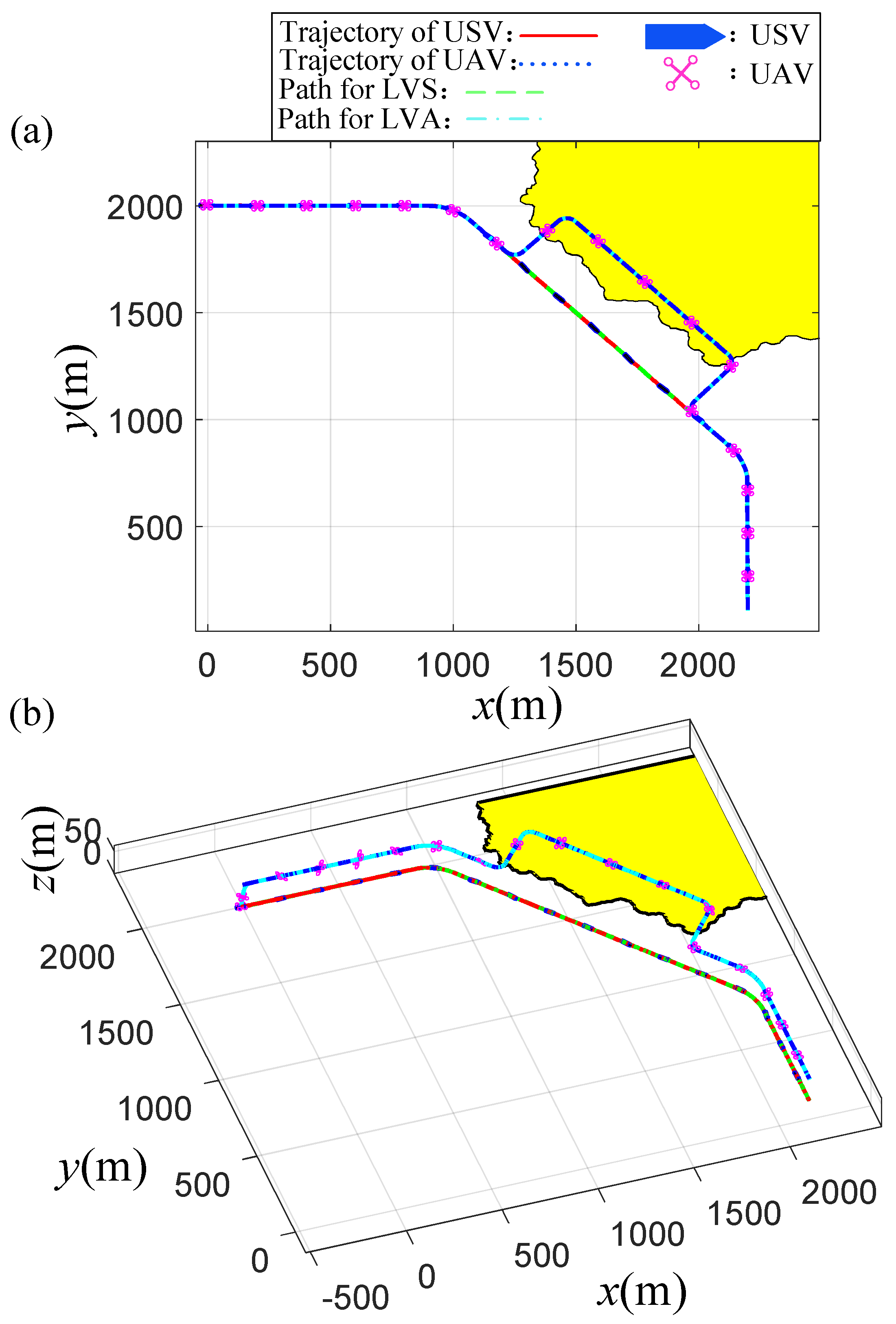
5.1. Guidance-based Simulation Experiment

In this experiment, the waypoints-based path-following experiment was performed. For this purpose, the reference path was generated by setting four waypoints $W_1$$\left(0 \mathrm{m} ,2000 \mathrm{m}\right)$, $W_2$$\left(1000 \mathrm{m}, 2000 \mathrm{m}\right)$, $W_3$$\left(2200 \mathrm{m}, 200 \mathrm{m}\right)$, and $W_4$$\left(2200 \mathrm{m}, 80 \mathrm{m}\right)$. To attain the objective of monitoring the shoreline, it is necessary to choose waypoints that are in close proximity to the shore whilst still enabling safe navigation. The initial states of the USV are expressed as $\left[x_s\left(0\right)\right.$, $y_s\left(0\right)$, ${\psi }_s\left(0\right)$, $u_s\left(0\right)$, $v_s\left(0\right)$, $\left.r_s\left(0\right)\right]$$=$$\left[-10\right. \mathrm{m}$, $2001 \mathrm{m}$, $17.2 \mathrm{deg}$, $0 \mathrm{m}/\mathrm{s}$, $0 \mathrm{m}/\mathrm{s}$, $\left.0 \mathrm{deg}/\mathrm{s}\right]$ and the initial states of UAV can be expressed as $\left[x_a\left(0\right)\right.$, $y_a\left(0\right)$, $z_a\left(0\right)$, ${\psi }_a\left(0\right)$, ${\varphi }_a\left(0\right)$, $\left.{\theta }_a\left(0\right)\right]$ = $\left[-5\right. \mathrm{m}$, $2005 \mathrm{m}$, $0 \mathrm{m}$, $0 \mathrm{deg}/\mathrm{s}$, $0 \mathrm{deg}/\mathrm{s}$, $\left.0 \mathrm{deg}/\mathrm{s}\right]$, the surge speed of LVS is chosen as $u_d=4 \mathrm{m}/\mathrm{s}$.

In this simulation, to show the marine environment more realistically, the physical-based mathematical model based on the NORSOK (Norwegian Standards Organization) wind spectrum and the JONSWAP (Joint North Sea Wave Observation Project) wave spectrum is employed. Specifically, the speed and direction of wind is $U_{tw}=4.75 \mathrm{m}/\mathrm{s}$ and ${\psi }_{tw}=20 \mathrm{deg}$. The JONSWAP wave spectrum is introduced to generate the time-varying wind-generated wave spectra with the third level of sea state. Furthermore, the design parameters and the adaptive parameters can be shown in (58).

$$\begin{array}{l}{k}_{ue}=5.1,k_{re}=3.7,k_u=130,k_r=6\times {10}^5,k_x=0.1,k_y=0.5,\\ k_z=10,k_{\psi }=17,k_{\varphi }=0.2,k_{\theta }=0.2,k_{\lambda \varsigma }^{}=k_{\lambda \sigma }^{}=1,\\ k_{\lambda }^{\varsigma }=k_{\lambda }^{\sigma }=0.05,k_{\mathrm{\Gamma }\varsigma }^{}=k_{\mathrm{\Gamma }\sigma }^{}=0.1,k_{\mathrm{\Gamma }}^{\varsigma }=k_{\mathrm{\Gamma }}^{\sigma }=1\times {10}^3\end{array}$$

(58)

Figure 5, Figure 6, Figure 7 and Figure 8 describe the main numerical results of the proposed algorithm under the marine environment. Figure 5 describes the trajectories for the USV-UAV system under the proposed guidance principle in different dimensions. Errors relating to the position loop and attitude loop can be obtained from Figure 6, however, when compared to the scale of the entire route, these errors are acceptable. Notably, the $x_{ae},y_{ae}$ change rapidly when they perform a separation and rendezvous, and eventually converge to zero, but ${\psi }_{ae}$ fluxes when the UAV is turning. Figure 7 and Figure 8 describe the control input for the USV and the UAV. The blue line represents the unquantized input signal and the red line represents the actual input signal after quantization. Similar to the ETC, the quantizer discretizes the continuous signals, one of which defines the quantification intervals and are similar to the triggering intervals. The stair-stepping phenomenon is evident in the quantitative part, which is similar to ETC.

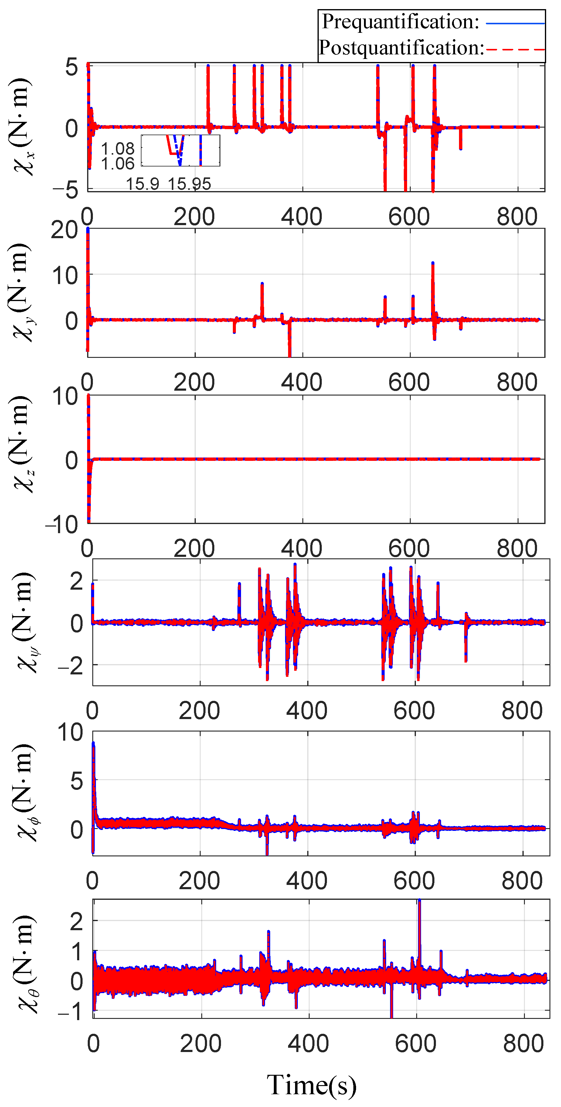
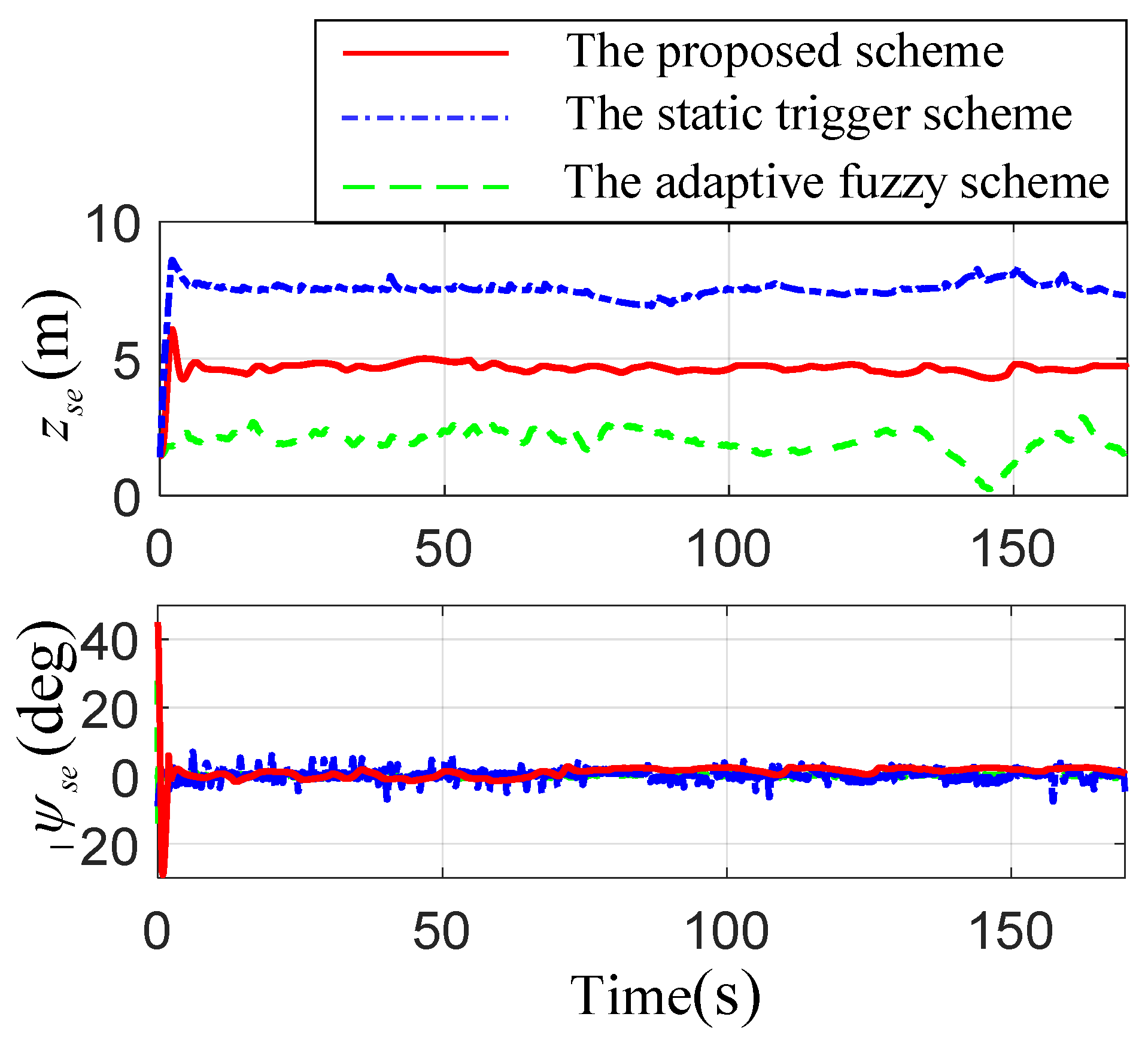
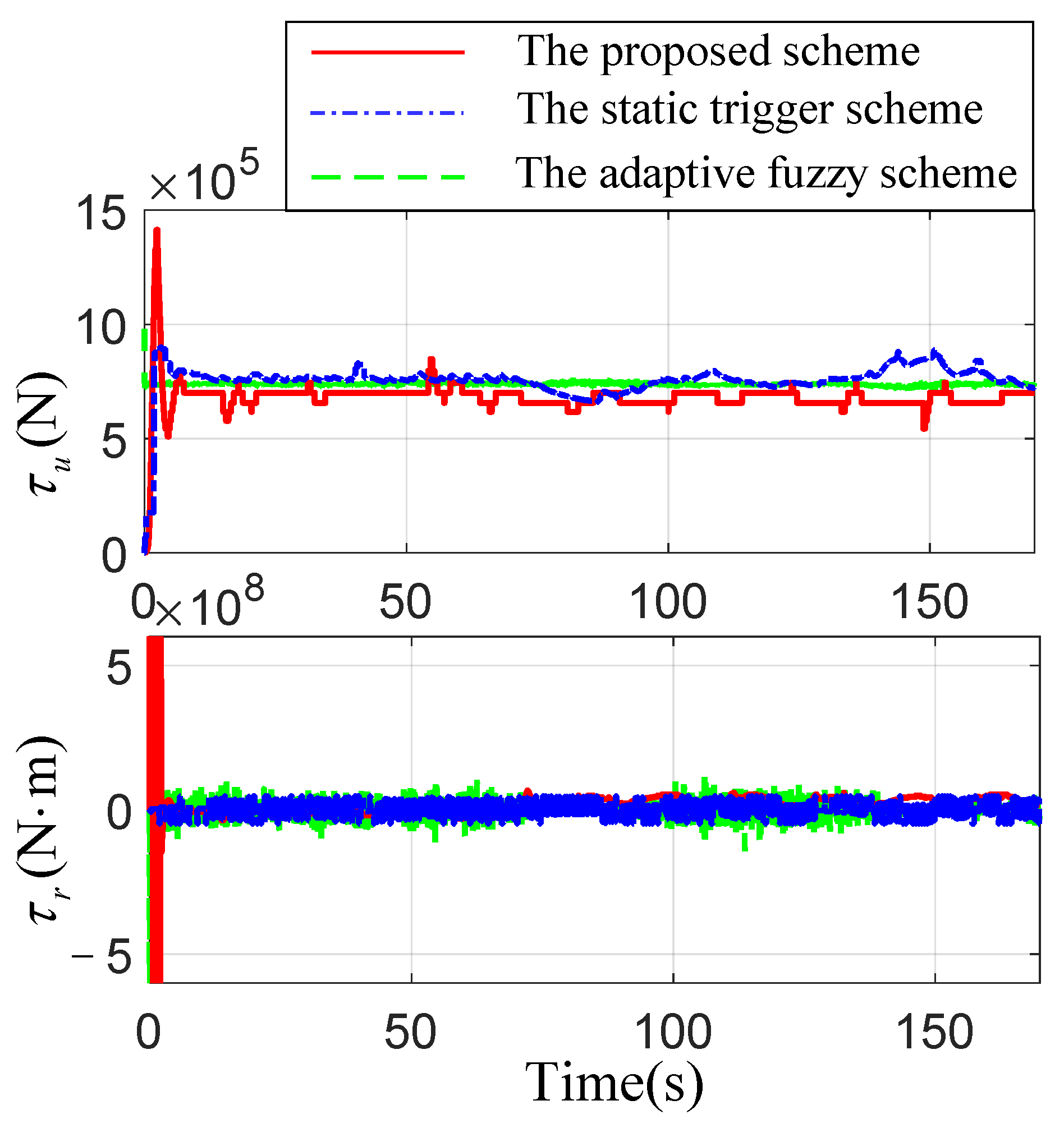
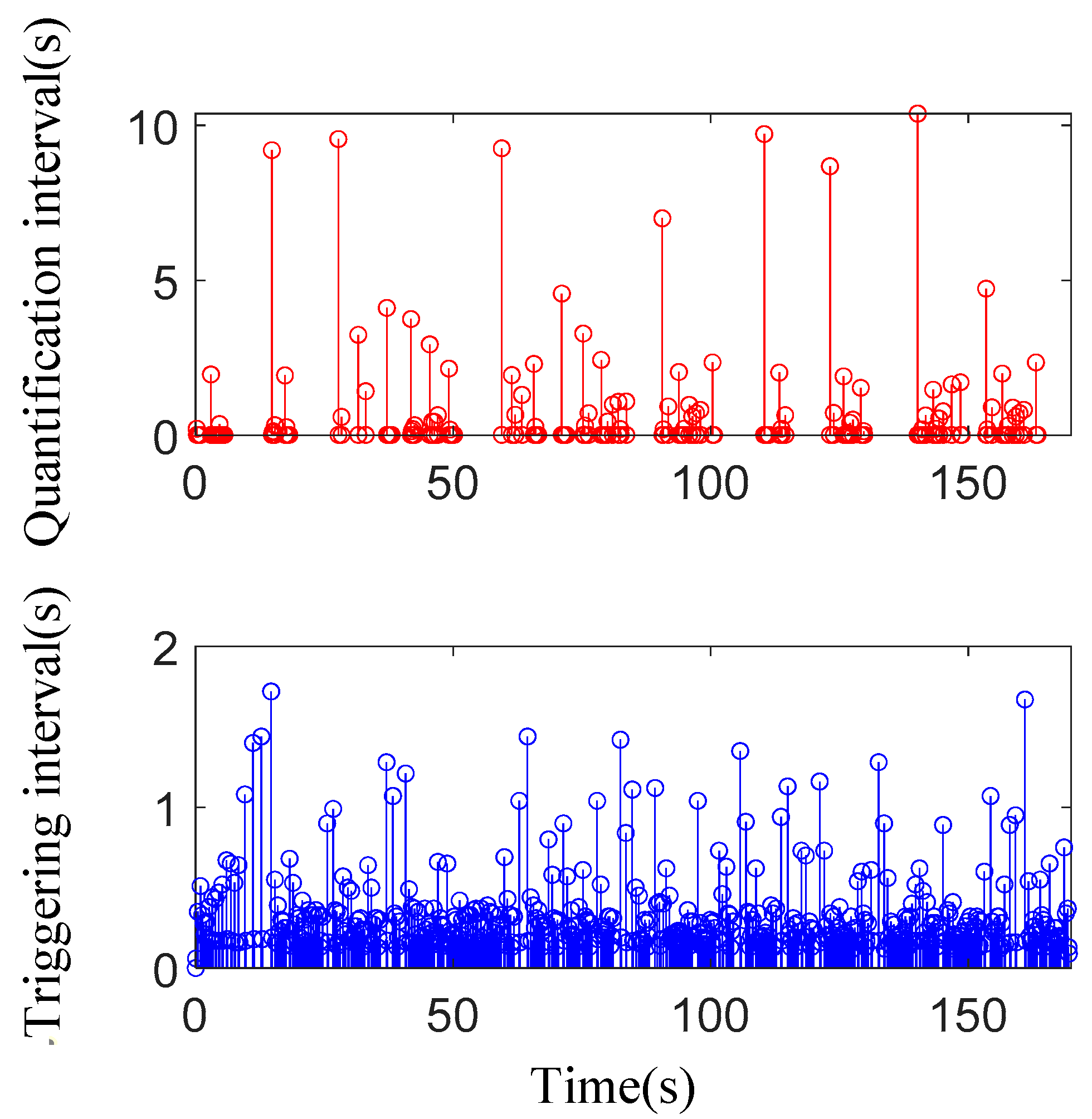
5.2. Comparative Experiment

In this subsection, the proposed adaptive fuzzy quantized control algorithm will be compared with the results in [41,42], which respectively are the static trigger scheme and adaptive fuzzy scheme mentioned below. To confirm the superiority in terms of robustness and control accuracy, a comparative experiment is conducted. The curved path is generated using the desired yaw velocities in (59) and the desired surge velocities $u_d=6.0 \mathrm{m}/\mathrm{s}$ with a sampling interval of 0.1 s. The JONSWAP wave spectrum is introduced to generate the time-varying wind-generated wave spectra with the third level of sea state. The underactuated ships initial states are set as $\left[x\left(0\right),y\left(0\right),\psi \left(0\right),\right.$$u\left(0\right),v\left(0\right),\left.r\left(0\right)\right]$ $=$ $\left[-1 \mathrm{m}, -1 \mathrm{m}, 0 \mathrm{deg}, 0 \mathrm{m}/\mathrm{s},\right.$ $\left.0 \mathrm{m}/\mathrm{s}, 0 \mathrm{rad}/\mathrm{s}\right]$.

$$r_d=\left\{\begin{array}{l}\exp \left(0.005t/300\right) \mathrm{rad}/\mathrm{s},t\in \left[0,30\right]\hfill \\ 0,t\in \left(30,70\right]\hfill \\ -0.05 \mathrm{rad}/\mathrm{s},t\in \left(70,170\right]\hfill \end{array}\right.$$

(59)

Therefore, the main comparative results are shown in Figure 9, Figure 10, Figure 11 and Figure 12. Figure 9 demonstrates the trajectories followed by three control algorithms when tracking the reference path, all of which exhibited satisfactory tracking accuracy. However, the proposed control algorithm has a higher tracking accuracy than the algorithm in [41] (see Figure 10). Figure 11 shows the control input under different control algorithms. Figure 10 is a comparison to [42], though the tracking accuracy is not especially favorable in the position loop, however it is satisfactory in the attitude loop. The reason the error in the position loop is of greater magnitude than in [42] is due to the small quantity which is added to ensure the LVS is ahead of the USV.

Figure 12 shows the quantification/triggering intervals along the voyage under the proposed algorithm and the algorithm in [41]. Notably, compared to the algorithm in [42], the proposed algorithm effectively reduces the communication frequency with minimal loss of error accuracy (see

Table 1. Quantitative results for the proposed scheme and [41,42].

Indexes	Items	The Proposed Algorithm	The Algorithm in [41]	The Algorithm in [42]
MAE	$z_{se}\left(\mathrm{m}\right)$	$4.6514$	$7.5154$	$1.9344$
	${\psi }_e\left(\mathrm{deg}\right)$	$1.6166$	$5.7898$	$2.5223$
MCI	${\tau }_u\left(\mathrm{N}\right)$	$6.8081\times {10}^5$	$7.5571\times {10}^5$	$7.3835\times {10}^5$
	${\tau }_r\left(\mathrm{N}\cdot \mathrm{m}\right)$	$2.6401\times {10}^7$	$5.5122\times {10}^7$	$6.0491\times {10}^7$
MVC	${\tau }_u\left(\mathrm{N}\right)$	$311.2944$	$5.5306\times {10}^3$	$2.6188\times {10}^3$
	${\tau }_r\left(\mathrm{N}\cdot \mathrm{m}\right)$	$181.8856$	$2.4439\times {10}^4$	$7.9108\times {10}^4$

). More specifically, (60) introduces three performance indexes as the metrics for assessing the effectiveness of the algorithm. The mean absolute error (MAE), the mean absolute control inputs (MCI), and the mean integrated variation of control inputs (MVC) describe the stabilization ability of the system, the energy consumption, and the responsiveness of system, respectively. The detailed quantitative results are illustrated in Table 1. Thereout, the proposed algorithm is with superior advantages of higher tracking accuracy and lower energy consumption.

$$\begin{array}{l}\mathrm{MAE}=\frac{1}{t_{end}-0}{\displaystyle {\int }_0^{t_{end}}\left|e\left(t\right)\right|dt}\hfill \\ \mathrm{MCI}=\frac{1}{t_{end}-0}{\displaystyle {\int }_0^{t_{end}}\left|\tau \left(t\right)\right|dt}\hfill \\ \mathrm{MVC}=\frac{1}{t_{end}-0}{\displaystyle {\int }_0^{t_{end}}\left|\tau \left(t+1\right)-\tau \left(t\right)\right|dt}\hfill \end{array}$$

(60)

6. Conclusions

An adaptive fuzzy quantized control algorithm has been developed for the implementation of the USV-UAV system based on asynchronous separate guidance principle, as well as considering the input quantization. Based on the waypoints, the proposed guidance principle removes time-restrictions when compared to previous guidance principles. The path planning in curved lines is calculated based on the velocity and the distance between the logic virtual vessel and the target point, which is more relevant to the actual situation as subsystems are fully utilized alongside the strong mobility and broad vision of the UAV and the high endurance of the USV. In addition, an adaptive fuzzy quantized control scheme considering a hysteretic quantizer was proposed and developed. This control algorithm can effectively reduce the conversion frequency of the control input variable, making it fluctuate in a stable range and reduce the execution times of the actuator, thus reducing actuator wear under conditions that satisfy the basic control requirements. The availability and advantages of the proposed strategy, namely in what concerns the lower command transmission and higher tracking accuracy requirements were evaluated using two numerical simulations. Nevertheless, this work cannot encompass all the details of the control task. For variables with large numerical values, quantization errors caused by quantifying the inputs may be significant.

Follow-up work will focus on gradually changing the UAV’s velocity whilst performing the separation and rendezvous tasks and the quantization errors.

References

1. Trejo, J.A.V.; Ponsart, J.-C.; Adam-Medina, M.; Valencia-Palomo, G.; Theilliol, D. Distributed Observer-based Leader-following Consensus Control for LPV Multi-agent Systems: Application to multiple VTOL-UAVs Formation Control. In Proceedings of the 2023 International Conference on Unmanned Aircraft Systems (ICUAS), Warsaw, Poland, 6–9 June 2023; pp. 1316–1323. [Google Scholar]
2. Zhang, B.; Ji, D.; Liu, S.; Zhu, X.; Xu, W. Autonomous underwater vehicle navigation: A review. Ocean Eng. 2023, 273, 113861. [Google Scholar] [CrossRef]
3. Zeng, Z.; Sammut, K.; Lian, L.; Lammas, A.; He, F.; Tang, Y. Rendezvous path planning for multiple autonomous marine vehicles. IEEE J. Ocean. Eng. 2018, 43, 640–664. [Google Scholar] [CrossRef]
4. Liu, B.; Zhang, H.-T.; Meng, H.; Fu, D.; Su, H. Scanning-Chain formation control for multiple unmanned surface vessels to pass through water channels. IEEE Trans. Cybern. 2022, 52, 1850–1861. [Google Scholar] [CrossRef]
5. Wu, Y.; Low, K.H.; Lv, C. Cooperative path planning for heterogeneous unmanned vehicles in a search-and-track mission aiming at an underwater target. IEEE Trans. Veh. Technol. 2020, 69, 6782–6787. [Google Scholar] [CrossRef]
6. Li, J.; Zhang, G.; Zhang, X.; Zhang, W. Integrating dynamic event-triggered and sensor-tolerant control: Application to USV-UAVs cooperative formation system for maritime parallel search. IEEE Trans. Intell. Transp. Syst. 2023, 1–13. [Google Scholar] [CrossRef]
7. Li, J.; Zhang, G.; Zhang, W.; Shan, Q.; Zhang, W. Cooperative path following control of USV-UAVs considering low design complexity and command transmission requirements. IEEE Trans. Intell. Veh. 2023, 1–10. [Google Scholar] [CrossRef]
8. Xiang, J.W.; Dong, X.W.; Ding, W.R. Key technologies for autonomous cooperation of unmanned swarm systems in complex environments. Acta Aeronaut. Astronaut. Sin. 2022, 43, 527570. [Google Scholar]
9. Duan, H.B.; Shen, Y.K.; Wang, Y.; Luo, D.; Niu, Y. Review of technological hotspots of unmanned aerial vehicle in 2018. Sci. Technol. Rev. 2019, 37, 82–90. [Google Scholar]
10. Fossen, T.I. Handbook of Marine Craft Hydrodynamics and Motion Control; John Wiley & Sons: Hoboken, NJ, USA, 2011; pp. 112–124. [Google Scholar]
11. Zhang, G.; Zhang, X. A novel DVS guidance principle and robust adaptive path-following control for underactuated ships using 473 low frequency gain-learning. ISA Trans. 2015, 56, 75–85. [Google Scholar] [CrossRef]
12. Li, J.; Zhang, G.; Shan, Q.; Zhang, W. A novel cooperative de sign for USV-UAV systems: 3D mapping guidance and adaptive fuzzy control. IEEE Trans. Control Netw. Syst. 2023, 10, 564–574. [Google Scholar] [CrossRef]
13. Zhang, H.-T.; Hu, B.-B.; Xu, Z.; Cai, Z.; Liu, B.; Wang, X.; Geng, T.; Zhong, S.; Zhao, J. Visual navigation and landing control of an unmanned aerial vehicle on a moving autonomous surface vehicle via adaptive learning. IEEE Trans. Neural Netw. Learn. Syst. 2021, 32, 5345–5355. [Google Scholar] [CrossRef] [PubMed]
14. Qin, S.; Yang, X.; Zhang, W.; Sun, M.; Liu, X.; Zhen, Z. Multi-target cooperative path planning for air-sea heterogeneous unmanned system. In Proceedings of the 2023 6th International Symposium on Autonomous Systems (ISAS), Nanjing, China, 23–25 June 2023; pp. 1–6. [Google Scholar]
15. Niu, H.; Ji, Z.; Liguori, P.; Yin, H.; Carrasco, J. Design, integration and sea trials of 3D printed unmanned aerial vehicle and unmanned surface vehicle for cooperative missions. In Proceedings of the 2021 IEEE/SICE International Symposium on System Integration (SII), Iwaki, Japan, 11–14 January 2021; pp. 590–591. [Google Scholar]
16. Liu, D.; Rong, H.; Soares, C.G. Shipping route modelling of AIS maritime traffic data at the approach to ports. Ocean Eng. 2023, 289, 115868. [Google Scholar] [CrossRef]
17. Liu, Z.; Huang, D.; Li, S.; Zhang, W.; Lu, H. Adaptive robust control of the UAV-USV heterogeneous system with unknown fractional-order dynamics under multiple disturbances. In Proceedings of the 2023 42nd Chinese Control Conference (CCC), Tianjin, China, 24–26 July 2023; pp. 5872–5877. [Google Scholar]
18. MahmoudZadeh, S.; Abbasi, A.; Yazdani, A.; Wang, H.; Liu, Y. Uninterrupted path planning system for Multi-USV sampling mission in a cluttered ocean environment. Ocean Eng. 2022, 254, 111328. [Google Scholar] [CrossRef]
19. Zhang, C.-L.; Guo, G. Prescribed performance fault-tolerant control of nonlinear systems via actuator switching. IEEE Trans. Fuzzy Syst. 2023, 1–10. [Google Scholar] [CrossRef]
20. Li, J.; Zhang, G.; Cabecinhas, D.; Pascoal, A.; Zhang, W. Prescribed performance path following control of USVs via an output-based threshold rule. IEEE Trans. Veh. Technol. 2023, 1–12. [Google Scholar] [CrossRef]
21. Zhang, G.; Li, J.; Jin, X.; Liu, C. Robust adaptive neural control for wing-sail-assisted vehicle via the multiport event-triggered approach. IEEE Trans. Cybern. 2022, 52, 12916–12928. [Google Scholar] [CrossRef]
22. Zhang, H.; Zhang, X.; Bu, R. Radial basis function neural network sliding mode control for ship path following based on position prediction. J. Mar. Sci. Eng. 2021, 9, 1055. [Google Scholar] [CrossRef]
23. Hua, C.-C.; Wang, K.; Chen, J.-N.; You, X. Tracking differentiator and extended state observer-based nonsingular fast terminal sliding mode attitude control for a quadrotor. Nonlinear Dyn. 2018, 94, 343–354. [Google Scholar] [CrossRef]
24. Swaroop, D.; Hedrick, J.K.; Yip, P.P.; Gerdes, J.C. Dynamic surface control for a class of nonlinear systems. IEEE Trans. Autom. Control 2000, 45, 1893–1899. [Google Scholar] [CrossRef]
25. Yu, J.L.; Dong, W.X.; Li, Q.D.; Ren, Z. Practical time-varying formation tracking for high-order nonlinear multi-agent systems based on the distributed extended state observer. Int. J. Control 2019, 92, 2451–2462. [Google Scholar] [CrossRef]
26. Liao, F.; Teo, R.; Wang, J.L.; Dong, X.; Lin, F.; Peng, K. Distributed Formation and Reconfiguration Control of VTOL UAVs. IEEE Trans. Control Syst. Technol. 2017, 25, 270–277. [Google Scholar] [CrossRef]
27. Zheng, Z.; Feroskhan, M. Path following of a surface vessel with prescribed performance in the presence of input saturation and external disturbances. IEEE/ASME Trans. Mechatron. 2017, 22, 2564–2575. [Google Scholar] [CrossRef]
28. Lili, W.; Chen, M. Distributed DETMs-based internal collision avoidance control for UAV formation with lumped disturbances. Appl. Math. Comput. 2022, 433, 127362. [Google Scholar]
29. Nuchkrua, T.; Leephakpreeda, T. Novel Compliant Control of a Pneumatic Artificial Muscle Driven by Hydrogen Pressure Under a Varying Environment. IEEE Trans. Ind. Electron. 2022, 69, 7120–7129. [Google Scholar] [CrossRef]
30. Hayakawaa, T.; Ishii, H.; Tsumurac, K. Adaptive quantized control for linear uncertain discrete-time systems. Automatica 2009, 45, 692–700. [Google Scholar] [CrossRef]
31. Hayakawaa, T.; Ishii, H.; Tsumurac, K. Adaptive quantized control for nonlinear uncertain systems. Syst. Control Lett. 2009, 58, 625–632. [Google Scholar] [CrossRef]
32. Zhou, J.; Wen, C.; Yang, G. Adaptive backstepping stabilization of nonlinear uncertain systems with quantized input signal. IEEE Trans. Autom. Control 2014, 59, 460–464. [Google Scholar] [CrossRef]
33. Yang, W.; Cui, G.; Yu, J.; Tao, C.; Li, Z. Finite-time adaptive fuzzy quantized control for a quadrotor UAV. IEEE Access 2020, 8, 179363–179372. [Google Scholar] [CrossRef]
34. Shao, G.; Ma, Y.; Malekian, R.; Yan, X.; Li, Z. A novel cooperative platform design for coupled USV-UAV systems. IEEE Trans. Ind. Inform. 2019, 15, 4913–4922. [Google Scholar] [CrossRef]
35. Ke, C.; Chen, H.F. Cooperative path planning for air-sea heterogeneous unmanned vehicles using search-and-tracking mission. Ocean. Eng. 2022, 262, 112020. [Google Scholar] [CrossRef]
36. Do, K. Practical control of underactuated ships. Ocean Eng. 2010, 37, 1111–1119. [Google Scholar] [CrossRef]
37. Eliker, K.; Zhang, W. Finite-time adaptive integral backstepping fast terminal sliding mode control application on quadrotor UAV. Int. J. Control Autom. Syst. 2020, 18, 415–430. [Google Scholar] [CrossRef]
38. Labbadi, M.; Cherkaoui, M. Robust adaptive backstepping fast terminal sliding mode controller for uncertain quadrotor UAV. Aerosp. Sci. Technol. 2019, 93, 105306. [Google Scholar] [CrossRef]
39. Liu, Z.; Wang, F.; Zhang, Y.; Chen, C.L.P. Fuzzy adaptive quantized control for a class of stochastic nonlinear uncertain systems. IEEE Trans. Cybern. 2016, 46, 524–534. [Google Scholar] [CrossRef] [PubMed]
40. Park, S.; Deyst, J.; How, J.P. A new nonlinear guidance logic for trajectory tracking. In Proceedings of the AIAA Guidance, Navigation, and Control Conference and Exhibit, Providence, RI, USA, 16–19 August 2004; Volume 2, pp. 941–956. [Google Scholar]
41. Wang, H.; Zhang, S. Event-triggered reset trajectory tracking control for unmanned surface vessel system. Proc. Inst. Mech. Eng. Part I J. Syst. Control Eng. 2021, 235, 633–645. [Google Scholar] [CrossRef]
42. Lin, X.; Nie, J.; Jiao, Y.; Liang, K.; Li, H. Adaptive fuzzy output feedback stabilization control for the underactuated surface vessel. Appl. Ocean Res. 2018, 74, 40–48. [Google Scholar] [CrossRef]
Figure 1. The force diagram considered for the cooperative USV-UAV system.
Jmse 11 02331 g001
Figure 2. The framework of the asynchronous separate guidance principle.
Jmse 11 02331 g002
Figure 3. The processes and details of the separation and rendezvous parts.
Jmse 11 02331 g003
Figure 4. The control framework for the USV-UAV system.
Jmse 11 02331 g004
Figure 5. Trajectories for the USV-UAV system under the proposed guidance principle: (a) 2D vertical view and (b) 3D space diagram.
Jmse 11 02331 g005
Figure 6. The position and heading errors for the USV-UAV system.
Jmse 11 02331 g006
Figure 7. Pre- and post-quantification control input for the USV.
Jmse 11 02331 g007
Figure 8. Pre- and post-quantification control input for the UAV.
Jmse 11 02331 g008
Figure 9. The comparison trajectories of USV under different control schemes.
Jmse 11 02331 g009
Figure 10. The position error and attitude error under different control schemes.
Jmse 11 02331 g010
Figure 11. The control input under different control schemes.
Jmse 11 02331 g011
Figure 12. Quantification intervals of the proposed scheme and triggering intervals of the scheme in [41].
Jmse 11 02331 g012