A Study on the Vibration Analysis of Thick-Walled, Fluid-Conveying Pipelines with Internal Hydrostatic Pressure

Abstract

Pipelines are designed to carry seawater with hydrostatic pressure below sea level in the ship industry. Previously conducted studies have established the FSI (Fluid–Structure Interaction) equations for thin-walled, fluid-filled pipelines based on the Timoshenko beam model; these equations now need to be modified for analyzing the vibration characteristics of thick-walled pipelines with hydrostatic pressure. The vibration of thick-walled pressurized pipes is studied in this paper. Effective and accurate numerical methods for solving vibration responses to either harmonic excitation or a random load have been developed using the spectral element method and pseudo-excitation method. It is found that the thick-walled theory and the thin-walled theory differ in axial wave transmissions. The internal pressure mainly affects the transverse vibration, which results in an increase in the natural frequencies in the lower frequency domain, an increase in the vibration transmission in the assembled pipeline, and an increase in the displacements when subjected to random loads. Using relatively thicker pipelines and introducing flexible pipes may reduce the vibration transmission when subjected to internal pressure.

1. Introduction

According to the ship pipeline design pressure classification, the design pressure of pipelines conveying water may exceed 4 MPa [1]. In addition, some pipelines are designed to carry seawater with hydrostatic pressure below sea level in military ships. When pipelines are suffering from hydrostatic pressure, pre-stress has been generated in these structures, even if evident damage has not been created. The pre-stress may change the natural frequencies and wave speed dispersion characteristics, so the vibration and sound characteristics will change afterwards. With increasing internal hydrostatic pressure, the vibration characteristics of pipes would obviously be changed [2]. In addition, the fluid flow increases in the pressurized pipes, which may cause the FSI (Fluid–Structure Interaction) to be more evident. Moreover, the vibration displacement amplitude increases along with the increasing flow velocity, which may easily induce the instability of the pipes. Though the flow velocity is usually controlled under the critical flow velocity, other phenomena, such as turbulence pulsation and vortex shedding [3], may induce time-varying forces on the pipes. These forces are considered to be one of the main causes of pipeline damage and failure. Therefore, it is necessary to investigate the vibration characteristics of fluid-conveying pipelines with internal hydrostatic pressure, which may provide theoretical support for the acoustic design optimization of ship pipe systems.

At present, most of the research on the vibration of pressurized pipes has mainly adopted the thin shell model. Fung [4] and Miserentino [5] investigated the impact of the internal hydrostatic pressure on the natural frequencies of thin-shelled cylindrical shells. Keltie [6] analyzed the vibration and sound radiation characteristics of cylindrical shells with internal hydrostatic pressure, compared the results with those without pressure, and concluded that the hydrostatic pressure and initial stresses will evidently affect the structural responses. Xie [7] added the hydrostatic pressure potential energy into the Hamilton’s variational equation and found that the variation in the vibration power is extremely complex with increasing hydrostatic pressure. Zhang [8] established the fluid-filled pre-stressed cylindrical shell model and analyzed the influence of initial tension, internal pressure, and fluid speed using the finite element method. Liu [9] considered the influence of static pressure on the dispersion characteristics of liquid-filled cylindrical shells. The results show that static pressure affects both the liquid-filled shell and the empty shell. With the cross-sectional shape changes, the impact of static pressure of the wave propagation also increases. Iakovlev [10] investigated fluid-filled cylindrical shells with internal hydrostatic pressure affected by external shocks and analyzed the sound velocity change on the structure. Chen [11] calculated the dynamic response of a cylindrical shell with local pre-stress using the structural finite element and acoustic boundary element methods. The existence of local pre-stress would change the local and general stiffness, which may lead to the change in the structural acoustic vibration characteristics. Gao [12,13] solved the fluid–structure coupled vibration of fluid-filled flexible pipes with flange support at both ends and verified the theoretical calculations through numerical simulation and experiments, which proves that static pressure also induces the initial stress and deformation in hoses.

However, most pipelines in engineering are three-dimensional structures, including several different kinds of pipes. Pipelines on ships are especially slender structures, which are more suitable to be modeled as beams. Neto et al. [14] simulated the computational model of the turbulent incompressible flow in conjunction with a Timoshenko beam in order to characterize the influence of the proximity of the seabed on the fluid–structure interaction using a simulation and theoretical analysis. Kiryukhin et al. [15] calculated the pressure pulsations and the induced dynamic loads in a liquid-filled pipeline, which were investigated through both experimental methods and mathematical models. Yamilev et al. [16] presented the Darcy–Weisbach formula for isothermal flows of a power-law fluid to perform simplified analytical thermal–hydraulic calculations for non-isothermal pipelines. Korshak et al. [17] proposed the computational fluid dynamic methods to simulate the process of water slug removal via the flow of pumped liquid in oil pipelines. The computed results are in high agreement with the data from experimental studies. Cao et al. [18] carried out vibration tests to investigate the acceleration response of the pipeline and pressure pulsation response of fluid when pipelines are subjected to internal fluid fluctuation excitation in the hydraulic pump and external excitations. These studies have not investigated and calculated the vibration and sound transmissions of pressurized pipelines with numerical methods.

The method of characteristics (MOC) was mainly adopted in a time domain analysis. Wiggert [19] solved the traditional FSI vibration equations (fourteen equations in 3D space) with the MOC and compared the results with experiments. Zhang and Tijsseling [20] calculated the transverse and axial vibrations of fluid-filled pipelines and then proved the response and natural frequency results through transverse and axial vibration experiments. The transfer matrix method (TMM), the finite element method (FEM), the impedance synthesis method (ISM), and the spectral element method (SEM) are mainly adopted in frequency domain analysis. When applying the TMM, the sub-transfer matrix of one pipe element was derived and these sub-transfer matrices were multiplied to form the whole transfer matrix. Lesmez [21], Tentarelli [22], Caf [23], Zhang [24], and Li [25] used Wiggert’s fourteen equations and TMM to solve the one-dimensional or two-dimensional vibrations of pipelines. The fluid–structure coupling and energy transmission were investigated in their study. Massive calculations of matrix multiplication were needed when dealing with long pipes, which may easily induce error accumulation. The finite element method (FEM) is one of the most popular numerical methods in engineering due to its wide application and simple modeling. Hansson [26] used axial symmetric shell elements and one-dimensional fluid elements to simulate the vibration of fluid-filled pipes. Everstine [27] investigated the dynamic responses of fluid-filled pipe systems with both a one-dimensional beam model and three-dimensional models using the finite element method. Lee [28] established the non-linear coupling equations for fluid-conveying pipelines based on the Euler beam model and derived the vibration solutions through the finite element method. Andreas et al. [29] used FEM analysis to establish a probabilistic fracture mechanics model to investigate the surface-cracked pipes subjected to tension load and internal pressure. Kainat et al. [30] studied the initial geometric imperfections on the bulking responses of high-strength pipes through the finite element analysis. Francis [31] proposed a fully Lagrangian finite element method to simulate the fluid–structure interactions, which obtained a good agreement with experimental results from the literature. Shahzamanian et al. [32] conducted a systematic literature review of experiments, analytical methods, FEM, and extended finite element methods (XFEM) to predict tensile failure in pipelines. XFEM has shown great promise for failure prediction of pipeline since XFEM avoids the need for mesh conformance to the crack geometry. Hicham et al. [33] studied the fluid–structure coupling between cylinders and internal laminar and incompressible fluids with the finite element method. Wu et al. [34] used the software Ansys Fluent 16.0 to analyze the pressure and velocity distribution of subsea tree oil pipelines and used the Ansys Workbench 16.0 to carry out flow–structure coupling calculations and modal analysis. Yu et al. [35] carried out the modal analysis experiments of fluid-filled pipelines with internal pressure. The influences of flow speed, internal pressure, joint effect, and pipe length on the vibration characteristics of multi-branched pipelines were analyzed through a finite element simulation. In a finite element analysis, the displacement functions are not accurate. The FSI problems usually require a large number of divided elements in order to derive accurate results, which may greatly reduce the computing efficiency. Zhu [36] developed the spectral element method and applied the SEM to 3D pipelines, including curved pipes and branch pipes. Wu [37,38] adopted the ISM to study the coupled vibration of pipelines installed on the assembled conical–cylindrical shells. While applying SEM or ISM, exact displacement functions were derived to formulate the element matrix. The accuracy of the results does not depend on the number of elements, which has shown great advantages in the calculation efficiency in the frequency domain, especially the higher frequency domain. The above research focused on the dynamic responses of thick-walled pipelines subjected to harmonic excitations.

In order to withstand the internal hydrostatic pressure, relatively thick pipelines are usually used in engineering. The impacts of hydrostatic pressure on the vibration and sound transmission of pipelines under harmonic or random loads have never been studied, which is the purpose of this paper. Lin [39,40] proposed the pseudo-excitation method for solving the dynamic responses of structures under random excitations. Suppose the power spectral density (PSD) of a stationary random excitation is known as $S_{ff}(\omega )$; then, the response of the structure could be determined with the pseudo-excitation method. A pseudo-harmonic excitation $\sqrt{S_{ff}\left(\omega \right)}{e}^{i\omega t}$ is given in order to calculate the pseudo-displacement $\tilde{u}$. The response self-power spectrum must be ${\tilde{u}}^{\ast }\tilde{u}$. Such a simplified procedure would greatly shorten the calculation difficulty of stochastic responses. Therefore, in this work, the spectral element method and pseudo-excitation method were adopted to calculate the harmonic and stochastic responses, which provides further understanding of the vibration and sound characteristics of fluid-conveying, thick-walled pressurized pipelines.

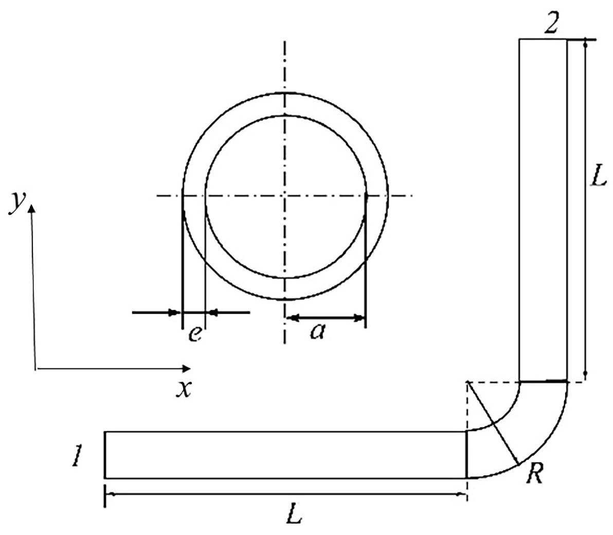
2. The Fluid–Structure Coupled Equation of Thick-Walled Pressurized Pipe in Plane

2.1. Vibration Equation of Pipe

The axial direction of the pipeline was the z-axis, and the transverse direction in the plane was the y-axis. We supposed that the angle between the axial direction and horizontal line was α. Therefore, the projections of gravity acceleration in the z-axis and y-axis directions were g_z = gsinα, g_y = gcosα. Based on the Timoshenko beam model, u(z,t) and w(z,t) (where t represents time) represented the axial displacement and transverse displacement, respectively. The rotation angle of the normal section was φ(z,t). The vertical and tangential forces acted on the internal fluid on the pipe wall of unit lengths are denoted by N_f and τ. The tension, shear force, and bending moment on the cross section were T(z,t), Q(z,t), and M(z,t), respectively.

The force analysis of an infinitesimal segment of pipeline is shown in Figure 1.

The equations for the axial and transverse motions were as follows:

$$\begin{array}{l}{T}^{\prime }+N_{\mathrm{f}}{w}^{\prime }+\tau -m_{\mathrm{p}}{g}_z=m_{\mathrm{p}}\ddot{u}\\ {\left(T{w}^{\prime }\right)}^{\prime }-Q^{\prime }-N_{\mathrm{f}}+\tau w^{\prime }-m_{\mathrm{p}}{g}_y=m_{\mathrm{p}}\ddot{w}\end{array},$$

(1)

where m_p was the mass of pipe with a per unit length, the superscript (’) represented $\partial /\partial z$, and (·) represented $\partial /\partial t$.

We supposed that the inner radius was R and the thickness was t. The sectional moment of inertia was $I_{\mathrm{p}}=\frac{\pi }{4}\left[{\left(R+t\right)}^4-R^4\right]$. The motion equation related to the rotation angle φ was as follows:

$${\rho }_{\mathrm{p}}{I}_{\mathrm{p}}\ddot{\phi }=M^{\prime }-Q,$$

(2)

where ρ_p was the density of the pipe.

2.2. Fluid Equations

Figure 2 shows the force analysis of an infinitesimal segment of fluid in the pipeline; p(z,t) and c(z,t) represented the fluid pressure and fluid velocity on the section, respectively; mf represented the mass of fluid with per unit length; and A_f was the sectional area of the fluid.

The momentum equations on the z and y directions were as follows:

$$\begin{array}{l}{p}^{\prime }{A}_{\mathrm{f}}+N_{\mathrm{f}}{w}^{\prime }+\tau +m_{\mathrm{f}}\left(g_z+\dot{c}+\ddot{u}+c{c}^{\prime }+c{\dot{u}}^{\prime }\right)=0\\ {\left(p{w}^{\prime }\right)}^{\prime }{A}_{\mathrm{f}}-N_{\mathrm{f}}+\tau w^{\prime }+m_{\mathrm{f}}\left(g_y+\ddot{w}+\dot{c}{w}^{\prime }+2c{\dot{w}}^{\prime }+c{c}^{\prime }{w}^{\prime }+c^2{w}^{″}\right)=0\end{array}.$$

(3)

The 2D continuum equation for the fluid in the pipeline was as follows:

$$\frac{1}{\mathrm{K}}\frac{\partial p}{\partial t}+\frac{\partial c}{\partial z}+\frac{2}{R}{\left.{\dot{u}}_r\right|}_{r=R}=0,$$

(4)

where K was the bulk modulus of fluid, and ${\left.{\dot{u}}_r\right|}_{r=R}$ represented the radial velocity on the cross section.

Introducing the constitutive equation ${\epsilon }_{\phi }=\frac{1}{\mathrm{E}}\left[{\sigma }_{\phi }-\mu \left({\sigma }_z+{\sigma }_r\right)\right]$ and geometric equation ${\epsilon }_{\phi }=\frac{u_r}{r}$, Equation (4) could be changed to the following:

$$\frac{1}{\mathrm{K}}\frac{\partial p}{\partial t}+\frac{\partial c}{\partial z}+\frac{2}{E}\frac{\partial }{\partial t}\left({\left.{\sigma }_{\phi }\right|}_{r=R}-\mu {\left.{\sigma }_z\right|}_{r=R}-\mu {\left.{\sigma }_r\right|}_{r=R}\right)=0.$$

(5)

The pipeline was under fluid pressure. Therefore, the axial stress was ${\left.{\sigma }_r\right|}_{r=R}=-p$, and the circumferential stress was ${\left.{\sigma }_{\phi }\right|}_{r=R}=\left(\frac{R}{e}+\frac{1+e/R}{2+e/R}\right)p$ [41]. The axial stress in the pipe section was considered to be consistent, which could be replaced by the average stress and ${\overline{\sigma }}_z{A}_{\mathrm{p}}=T$. Equation (5) was rewritten as follows:

$$\frac{\partial c}{\partial z}+\left[\frac{1}{\mathrm{K}}+\frac{2}{\mathrm{E}}\left(\frac{R}{e}+\frac{1+e/R}{2+e/R}+\mu \right)\right]\frac{\partial p}{\partial t}=\frac{2\mu }{\mathrm{E}}\frac{\partial {\overline{\sigma }}_z}{\partial t}.$$

(6)

The axial constitutive equation and geometric equations were ${\epsilon }_z=\frac{1}{\mathrm{E}}\left[{\sigma }_z-\mu \left({\sigma }_{\phi }+{\sigma }_r\right)\right]$ and ${\epsilon }_z=\frac{\partial u_z}{\partial z}$, which indicated the following:

$${\overline{\sigma }}_z=E\frac{\partial {\overline{u}}_z}{\partial z}+\mu \left({\overline{\sigma }}_{\phi }+{\overline{\sigma }}_r\right).$$

(7)

In elasticity [42], the stresses on the cross section of a cylindrical shell with internal pressure satisfied ${\overline{\sigma }}_{\phi }+{\overline{\sigma }}_r=\frac{R}{e}\frac{1}{1+\frac{1}{2}\frac{e}{R}}p$. Equation (6) was formed as follows:

$$\frac{\partial c}{\partial z}+\left[\frac{1}{\mathrm{K}}+\frac{2}{\mathrm{E}}\left(\frac{R}{e}\left(1-\frac{{\mu }^2}{1+\frac{1}{2}\frac{e}{R}}\right)+\frac{1+e/R}{2+e/R}+\mu \right)\right]\frac{\partial p}{\partial t}=2\mu \frac{{\partial }^2{u}_z}{\partial t\partial z}.$$

(8)

It was supposed that the axial displacements on the same cross section were consistent; therefore, $u_z$ and ${\overline{u}}_z$ were the same. The displacement u in Section 2.1 was u_z in this section, which was used to distinguish the axial and radial displacements.

2.3. The Governing FSI Equations for Pressurized Thick-Walled Pipeline

The axial and circumferential pre-stress in the pipe induced by internal hydrostatic pressure were as follows [43]:

$${\sigma }_{zz}^0=\frac{p_{0}R}{2t},{\sigma }_{\theta \theta }^0=\frac{p_{0}R}{t}.$$

(9)

The axial pre-stress could induce initial tension $T_0=\frac{p_{0}R}{2t}{A}_{\mathrm{p}}$, while the effect of circumferential pre-stress has been counted in Section 2.2. According to Timoshenko’s beam theory, the tension, shear force, and moment on the cross section are, respectively, as follows:

$$T=E{A}_{\mathrm{p}}{u}^{\prime }+T_0,Q=k_{\mathrm{s}}G{A}_{\mathrm{p}}\left(\phi -w^{\prime }\right)-T_0{w}^{\prime },M=E{I}_{\mathrm{p}}{\phi }^{\prime },$$

(10)

where k_s is the shear coefficient.

The fluid velocity and pressure were assumed to be linear:

$$c\left(z,t\right)=c_0+c_{\mathrm{d}}\left(z,t\right)p\left(z,t\right)=p_0+p_{\mathrm{d}}\left(z,t\right),$$

(11)

where subscript 0 meant the stationary value, and subscript d meant the average pulsation value.

Within the circular pipe, the friction between the fluid and pipe wall was (White 2005) $\tau =m_{\mathrm{f}}\frac{f_s}{2D}{c}^2$, where f_s was the friction coefficient and D the inner diameter.

Equations (1)–(3) and (8) were summarized as follows:

$$\begin{array}{l}E{A}_{\mathrm{p}}{u}^{″}+m_{\mathrm{f}}{g}_y{w}^{\prime }+m_{\mathrm{f}}\frac{f_{\mathrm{s}}}{D}{c}_0{\dot{v}}_{\mathrm{f}}=m_{\mathrm{p}}\ddot{u}\\ T_0{w}^{″}+k_{\mathrm{s}}G{A}_{\mathrm{p}}\left(w^{″}-{\phi }^{\prime }\right)-p_0{A}_{\mathrm{f}}{w}^{″}-m_{\mathrm{f}}\left(c_0{}^2{w}^{″}+2c_0{\dot{w}}^{\prime }+\ddot{w}\right)=m_{\mathrm{p}}\ddot{w}\\ {\rho }_{\mathrm{p}}{I}_{\mathrm{p}}\ddot{\phi }=E{I}_{\mathrm{p}}{\phi }^{″}-k_{\mathrm{s}}G{A}_{\mathrm{p}}\left(\phi -w^{\prime }\right)+T_0{w}^{\prime }\\ {p^{\prime }}_{\mathrm{d}}{A}_{\mathrm{f}}+m_{\mathrm{f}}{g}_y{w}^{\prime }+m_{\mathrm{f}}\frac{f_{\mathrm{s}}}{D}{c}_0{\dot{v}}_{\mathrm{f}}+m_{\mathrm{f}}\left(g_z+{\ddot{v}}_{\mathrm{f}}+\ddot{u}+c_0{{\dot{v}}^{\prime }}_{\mathrm{f}}+c_0{\dot{u}}^{\prime }\right)=0\\ \frac{\partial p_{\mathrm{d}}}{\partial t}+K^{\ast }\frac{\partial {\dot{v}}_{\mathrm{f}}}{\partial z}-2\mu K^{\ast }\frac{{\partial }^{2}u}{\partial t\partial z}=0\end{array},$$

(12)

where v_f was the fluid displacement, i.e., ${\dot{v}}_{\mathrm{f}}=c_{\mathrm{d}}$, and $K^{*}={\left(\frac{1}{K}+\frac{2}{E}\left[\frac{R}{e}\left(1-\frac{{\mu }^2}{1+\frac{e}{2R}}\right)+\frac{1+\frac{e}{R}}{2+\frac{e}{R}}+\mu \right]\right)}^{-1}$.

We supposed the variables in Equation (12) were in the following forms:

$$\begin{array}{l}u\left(z,t\right)=U\left(z\right){\mathrm{e}}^{\mathrm{i}\omega t},w\left(z,t\right)=W\left(z\right){\mathrm{e}}^{\mathrm{i}\omega t},\phi \left(z,t\right)=\Phi \left(z\right){\mathrm{e}}^{\mathrm{i}\omega t}\\ v_{\mathrm{f}}\left(z,t\right)=V_{\mathrm{f}}\left(z\right){\mathrm{e}}^{\mathrm{i}\omega t},p_{\mathrm{d}}\left(z,t\right)=P_{\mathrm{d}}\left(z\right){\mathrm{e}}^{\mathrm{i}\omega t}\end{array},$$

(13)

where i was the imaginary unit (i.e., ${\mathrm{i}}^2=-1$) and ω was the circular frequency.

The first four equations in Equation (12) were used to calculate the axial and transverse vibration. They were expressed in matrix form as follows:

$$\left[\begin{array}{cccc}{a}_1\frac{{\partial }^2}{\partial z^2}+a_2& a_3\frac{\partial }{\partial z}& 0& a_4\\ 0& a_5\frac{{\partial }^2}{\partial z^2}+a_6\frac{\partial }{\partial z}+a_7& a_8\frac{\partial }{\partial z}& 0\\ 0& a_9\frac{\partial }{\partial z}& a_{10}\frac{{\partial }^2}{\partial z^2}+a_{11}\frac{\partial }{\partial z}& 0\\ a_{12}\frac{{\partial }^2}{\partial z^2}+a_{13}\frac{\partial }{\partial z}+a_{14}& a_{15}\frac{\partial }{\partial z}& 0& a_{16}\frac{{\partial }^2}{\partial z^2}+a_{17}\frac{\partial }{\partial z}+a_{18}\end{array}\right]\left[\begin{array}{c}U\\ W\\ \Phi \\ V_{\mathrm{f}}\end{array}\right]=0,$$

(14)

where the coefficients were as follows:

$$\begin{array}{l}{a}_1=E{A}_{\mathrm{p}},a_2=m_{\mathrm{p}}{\omega }^2,a_3=m_{\mathrm{f}}{g}_y,a_4=m_{\mathrm{f}}\frac{f_s}{D}{c}_0\mathrm{i}\omega ,a_5=T_0+k_{s}G{A}_{\mathrm{p}}-p_0{A}_{\mathrm{f}}-m_{\mathrm{f}}{c}_0{}^2,a_6=-2m_{\mathrm{f}}{c}_0\mathrm{i}\omega ,\\ a_7=\left(m_{\mathrm{f}}+m_{\mathrm{p}}\right){\omega }^2,a_8=-k_{s}G{A}_{\mathrm{p}},a_9=k_{s}G{A}_{\mathrm{p}}+T_0,a_{10}=E{I}_{\mathrm{p}},a_{11}=-k_{s}G{A}_{\mathrm{p}}+{\rho }_{\mathrm{p}}{I}_{\mathrm{p}}{\omega }^2,\\ a_{12}=2\mu K^{\ast }\mathrm{i}\omega A_{\mathrm{f}},a_{13}=-m_{\mathrm{f}}{c}_0{\omega }^2,a_{14}=-m_{\mathrm{f}}\mathrm{i}{\omega }^3,a_{15}=m_{\mathrm{f}}{g}_{y}i\omega ,a_{16}=-K^{\ast }{A}_{\mathrm{f}}\mathrm{i}\omega ,a_{17}=-m_{\mathrm{f}}{c}_0{\omega }^2,\\ a_{18}=\left(-\mathrm{i}{\omega }^3-\frac{f_s}{D}{c}_0{\omega }^2\right)m_{\mathrm{f}}\end{array}$$

The solutions to Equation (14) were supposed to be in the forms $U={\displaystyle \sum _{j=1}^8{A}_j{\mathrm{e}}^{\mathrm{i}{\lambda }_{j}z}}$, $W={\displaystyle \sum _{j=1}^8{B}_j{\mathrm{e}}^{\mathrm{i}{\lambda }_{j}z}}$, $\Phi ={\displaystyle \sum _{j=1}^8{C}_j{\mathrm{e}}^{\mathrm{i}{\lambda }_{j}z}}$, $V_{\mathrm{f}}={\displaystyle \sum _{j=1}^8{D}_j{\mathrm{e}}^{\mathrm{i}{\lambda }_{j}z}}$, which could be inserted into Equation (14). Then, the determinant related to ${\lambda }_j$ was as follows:

$$\left|\begin{array}{cccc}-a_1{\lambda }_j^2+a_2& a_3\mathrm{i}{\lambda }_j& 0& a_4\\ 0& -a_5{\lambda }_j^2+a_6\mathrm{i}{\lambda }_j+a_7& a_8\mathrm{i}{\lambda }_j& 0\\ 0& a_9\mathrm{i}{\lambda }_j& -a_{10}{\lambda }_j^2+a_{11}\mathrm{i}{\lambda }_j& 0\\ -a_{12}{\lambda }_j^2+a_{13}\mathrm{i}{\lambda }_j+a_{14}& a_{15}i{\lambda }_j& 0& -a_{16}{\lambda }_j^2+a_{17}\mathrm{i}{\lambda }_j+a_{18}\end{array}\right|=0.$$

(15)

Eight roots were derived, written as ${\lambda }_1-{\lambda }_8$. Meanwhile, the relations between the coefficients were $A_j=u_j{C}_j,B_j=w_j{C}_j,D_j=f_j{C}_j$ (u_j, w_j, f_j could be derived through rank relation in Equation (15)).

We set a pipeline with length L as a pipe element; the displacements on the two ends were as follows:

$$\begin{array}{c}{U}_{z1}=U\left(0\right), U_{y1}=W\left(0\right), {\Phi }_1=\Phi \left(0\right)V_{f1}=V_f\left(0\right)\\ U_{z2}=U\left(L\right), U_{y2}=W\left(L\right), {\Phi }_2=\Phi \left(L\right),V_{f2}=V_f\left(L\right).\end{array}$$

(16)

The displacements were expressed in matrix form as follows:

$$\left[\begin{array}{c}{U}_{z1}\\ U_{y1}\\ {\Phi }_1\\ V_{\mathrm{f}1}\\ U_{z2}\\ U_{y2}\\ {\Phi }_2\\ V_{\mathrm{f}2}\end{array}\right]=\left[\begin{array}{cccccccc}{u}_1& u_2& u_3& u_4& u_5& u_6& u_7& u_8\\ w_1& w_2& w_3& w_4& w_5& w_6& w_7& w_8\\ 1& 1& 1& 1& 1& 1& 1& 1\\ f_1& f_2& f_3& f_4& f_5& f_6& f_7& f_8\\ u_1{e}^{\mathrm{i}{\lambda }_{1}L}& u_2{e}^{\mathrm{i}{\lambda }_{2}L}& u_3{e}^{\mathrm{i}{\lambda }_{3}L}& u_4{e}^{\mathrm{i}{\lambda }_{4}L}& u_5{e}^{\mathrm{i}{\lambda }_{5}L}& u_6{e}^{\mathrm{i}{\lambda }_{6}L}& u_7{e}^{\mathrm{i}{\lambda }_{7}L}& u_8{e}^{\mathrm{i}{\lambda }_{8}L}\\ w_1{e}^{\mathrm{i}{\lambda }_{1}L}& w_2{e}^{\mathrm{i}{\lambda }_{2}L}& w_3{e}^{\mathrm{i}{\lambda }_{3}L}& w_4{e}^{\mathrm{i}{\lambda }_{4}L}& w_5{e}^{\mathrm{i}{\lambda }_{5}L}& w_6{e}^{\mathrm{i}{\lambda }_{6}L}& w_7{e}^{\mathrm{i}{\lambda }_{7}L}& w_8{e}^{\mathrm{i}{\lambda }_{8}L}\\ e^{\mathrm{i}{\lambda }_{1}L}& e^{\mathrm{i}{\lambda }_{2}L}& e^{\mathrm{i}{\lambda }_{3}L}& e^{\mathrm{i}{\lambda }_{4}L}& e^{\mathrm{i}{\lambda }_{5}L}& e^{\mathrm{i}{\lambda }_{6}L}& e^{\mathrm{i}{\lambda }_{7}L}& e^{\mathrm{i}{\lambda }_{8}L}\\ f_1{e}^{\mathrm{i}{\lambda }_{1}L}& f_2{e}^{\mathrm{i}{\lambda }_{2}L}& f_3{e}^{\mathrm{i}{\lambda }_{3}L}& f_4{e}^{\mathrm{i}{\lambda }_{4}L}& f_5{e}^{\mathrm{i}{\lambda }_{5}L}& f_6{e}^{\mathrm{i}{\lambda }_{6}L}& f_7{e}^{\mathrm{i}{\lambda }_{7}L}& f_8{e}^{\mathrm{i}{\lambda }_{8}L}\end{array}\right]\left[\begin{array}{c}{C}_1\\ C_2\\ C_3\\ C_4\\ C_5\\ C_6\\ C_7\\ C_8\end{array}\right].$$

(17)

We inserted the displacement functions into Equation (10), and the forces on the cross section were as follows:

$$\begin{array}{l}T=E{A}_{\mathrm{p}}{u}^{\prime }={\displaystyle \sum _{j=1}^8{t}_j{C}_j{\mathrm{e}}^{\mathrm{i}{\lambda }_{j}z}}{\mathrm{e}}^{\mathrm{i}\omega t},p_{\mathrm{d}}=2\mu K^{\ast }{u}^{\prime }-K^{\ast }{v^{\prime }}_{\mathrm{f}}={\displaystyle \sum _{j=1}^8{p}_j{C}_j{\mathrm{e}}^{\mathrm{i}{\lambda }_{j}z}}{\mathrm{e}}^{\mathrm{i}\omega t}\\ Q=ksG{A}_{\mathrm{p}}\left(\phi -w^{\prime }\right)-T_0{w}^{\prime }={\displaystyle \sum _{j=1}^8{q}_j{C}_j{e}^{\mathrm{i}{\lambda }_{j}z}{\mathrm{e}}^{\mathrm{i}\omega t}},M=E{I}_{\mathrm{p}}{\phi }^{\prime }={\displaystyle \sum _{j=1}^8{m}_j{C}_j{\mathrm{e}}^{\mathrm{i}{\lambda }_{j}z}{\mathrm{e}}^{\mathrm{i}\omega t}}\end{array},$$

(18)

where

$$\begin{gathered} t_j=E{A}_{\mathrm{p}}{u}_j(i{\lambda }_j),p_j=2\mu K^{\ast }{u}_j\left(i{\lambda }_j\right)-K^{\ast }{f}_j\left(i{\lambda }_j\right), \\ {q}_j=ksG{A}_p\left(1-w_j\mathrm{i}{\lambda }_j\right)-T_0{w}_j\mathrm{i}{\lambda }_j,m_j=E{I}_p\mathrm{i}{\lambda }_j. \end{gathered}$$

As shown in Figure 3, the nodal forces on the ends of the pipe element were as follows:

$$\begin{array}{l}{F}_{z1}=-T\left(0\right), F_{y1}=-Q\left(0\right), M_1=-M\left(0\right), P_{d1}=-P_d\left(0\right)\\ F_{z2}=T\left(L\right), F_{y2}=Q\left(L\right), M_2=M\left(L\right), P_{d2}=P_d\left(L\right).\end{array}$$

(19)

The nodal forces were expressed in matrix form as follows:

$$\left[\begin{array}{c}{F}_{z1}\\ F_{y1}\\ M_1\\ P_{d1}\\ F_{z2}\\ F_{y2}\\ M_2\\ P_{d2}\end{array}\right]=\left[\begin{array}{cccccccc}-t_1& -t_2& -t_3& -t_4& -t_5& -t_6& -t_7& -t_8\\ -q_1& -q_2& -q_3& -q_4& -q_5& -q_6& -q_7& -q_8\\ -m_1& -m_2& -m_3& -m_4& -m_5& -m_6& -m_7& -m_8\\ -p_1& -p_2& -p_3& -p_4& -p_5& -p_6& -p_7& -p_8\\ t_1{\mathrm{e}}^{\mathrm{i}{\lambda }_{1}L}& t_2{\mathrm{e}}^{\mathrm{i}{\lambda }_{2}L}& t_3{\mathrm{e}}^{\mathrm{i}{\lambda }_{3}L}& t_4{\mathrm{e}}^{\mathrm{i}{\lambda }_{4}L}& t_5{\mathrm{e}}^{\mathrm{i}{\lambda }_{5}L}& t_6{\mathrm{e}}^{\mathrm{i}{\lambda }_{6}L}& t_7{\mathrm{e}}^{\mathrm{i}{\lambda }_{7}L}& t_8{\mathrm{e}}^{\mathrm{i}{\lambda }_{8}L}\\ q_1{\mathrm{e}}^{\mathrm{i}{\lambda }_{1}L}& q_2{\mathrm{e}}^{\mathrm{i}{\lambda }_{2}L}& q_3{\mathrm{e}}^{\mathrm{i}{\lambda }_{3}L}& q_4{\mathrm{e}}^{\mathrm{i}{\lambda }_{4}L}& q_5{\mathrm{e}}^{\mathrm{i}{\lambda }_{5}L}& q_6{\mathrm{e}}^{\mathrm{i}{\lambda }_{6}L}& q_7{\mathrm{e}}^{\mathrm{i}{\lambda }_{7}L}& q_8{\mathrm{e}}^{\mathrm{i}{\lambda }_{8}L}\\ m_1{\mathrm{e}}^{\mathrm{i}{\lambda }_{1}L}& m_2{\mathrm{e}}^{\mathrm{i}{\lambda }_{2}L}& m_3{\mathrm{e}}^{\mathrm{i}{\lambda }_{3}L}& m_4{\mathrm{e}}^{\mathrm{i}{\lambda }_{4}L}& m_5{\mathrm{e}}^{\mathrm{i}{\lambda }_{5}L}& m_6{\mathrm{e}}^{\mathrm{i}{\lambda }_{6}L}& m_7{\mathrm{e}}^{\mathrm{i}{\lambda }_{7}L}& m_8{\mathrm{e}}^{\mathrm{i}{\lambda }_{8}L}\\ p_1{\mathrm{e}}^{\mathrm{i}{\lambda }_{1}L}& p_2{\mathrm{e}}^{\mathrm{i}{\lambda }_{2}L}& p_3{\mathrm{e}}^{\mathrm{i}{\lambda }_{3}L}& p_4{\mathrm{e}}^{\mathrm{i}{\lambda }_{4}L}& p_5{\mathrm{e}}^{\mathrm{i}{\lambda }_{5}L}& p_6{\mathrm{e}}^{\mathrm{i}{\lambda }_{6}L}& p_7{\mathrm{e}}^{\mathrm{i}{\lambda }_{7}L}& p_8{\mathrm{e}}^{\mathrm{i}{\lambda }_{8}L}\end{array}\right]\left[\begin{array}{c}{C}_1\\ C_2\\ C_3\\ C_4\\ C_5\\ C_6\\ C_7\\ C_8\end{array}\right].$$

(20)

Equation (20) could be rewritten in the vector form as follows:

$$\begin{array}{l}\mathit{W} = {\mathit{K}}_{\mathbf{1}}\mathit{C}\\ \mathit{F} = {\mathit{K}}_{\mathbf{2}}\mathit{C}\end{array}.$$

(21)

Then, the nodal forces and displacements were related to the spectral element matrix:

$$\mathit{F}={\mathit{K}}_{\mathrm{d}}\mathit{W},$$

(22)

where ${\mathit{K}}_{\mathrm{d}}^{}={\mathit{K}}_2{\mathit{K}}_1{}^{-1}$ was the spectral element matrix in the y–z plane.

If several nodal displacements were restricted, boundary conditions were applied by setting the corresponding diagonal elements in K_d as large values. When the determinant of ${\mathit{K}}_{\mathrm{d}}$ reached its extremum, the corresponding frequency was the natural frequency. When external forces F were applied, the corresponding displacement response was $\mathit{W} = {\mathit{K}}_d{}^{-1}\mathit{F}$. The pipe elements could be assembled through the finite element method, which could be used to calculate the vibration of the assembled pipes. Compared with the finite element method, the exact displacement functions were used in the spectral element method. Therefore, unless the geometry shape or pipe material changes, only one element was enough for the vibration calculation. However, one more node needed to be added in the condition of pipelines with both ends clamped.

2.4. Pseudo-Excitation Method for Pipes Subjected to Random Loads

The pipeline was subjected to a randomly varying force at a specific location; for example, $f(t)$ was acting on the specific location z = z₀. The power spectral density (PSD) of a stationary random excitation was known as $S_{ff}(\omega )$. In this case, the pipeline needed to be divided into two elements. The expression $\sqrt{S_{ff}\left(\omega \right)}{e}^{i\omega t}$ would be the pseudo-nodal force on the middle nodal; then, the corresponding nodal displacements $\tilde{u}$ were the pseudo-displacements, which could be used to calculate the self-power spectrum, i.e., ${\tilde{u}}^{\ast }\tilde{u}$.

When the pipeline was subjected to a distributed randomly varying loading. The exciting force $f(z,t)$ could be written as follows:

$$f\left(z,t\right)=f_0\left(z\right)\theta \left(t\right),$$

where $\theta \left(t\right)$ was a stochastic process, whose PSD of this stationary random excitation was $S_{\theta }(\omega )$.

In order to derive the pseudo-displacement, a shape function was introduced. We let $W\left(z\right)$ represent the transverse displacement function. Then, the following was derived:

$$W\left(z\right)=\mathit{N}{\mathit{d}}^{\mathrm{e}},$$

(23)

where N was the shape function, and ${\mathit{d}}^{\mathrm{e}}$ represented the nodal displacement column vector. According to Section 2.3, N and ${\mathit{d}}^{\mathrm{e}}$ were in the following forms:

$$\mathit{N}=\left[\begin{array}{cccccccc}{w}_1{e}^{i{\lambda }_{1}z}& w_2{e}^{i{\lambda }_{2}z}& w_3{e}^{i{\lambda }_{3}z}& w_4{e}^{i{\lambda }_{4}z}& w_5{e}^{i{\lambda }_{5}z}& w_6{e}^{i{\lambda }_{6}z}& w_7{e}^{i{\lambda }_{7}z}& w_8{e}^{i{\lambda }_{8}z}\end{array}\right]{\mathit{K}}_1^{-1},$$

$${\mathit{d}}^e=\left[\begin{array}{cccccccc}{U}_{z1}& U_{y1}& {\varphi }_1& V_{\mathrm{f}1}& U_{z2}& U_{y2}& {\varphi }_2& V_{\mathrm{f}2}\end{array}\right].$$

The nodal force column vector was derived by the following:

$$f^{\mathrm{e}}={\displaystyle {\int }_0^L{f}_0\left(z\right)\sqrt{S_{\theta }(\omega )}}{N}^{\mathrm{T}}d\mathrm{z}.$$

(24)

We set $f^{\mathrm{e}}$ as the external force; the pseudo-nodal displacements were derived through Equation (22). Then, the self-power spectrum could be easily derived.

3. Results and Discussion

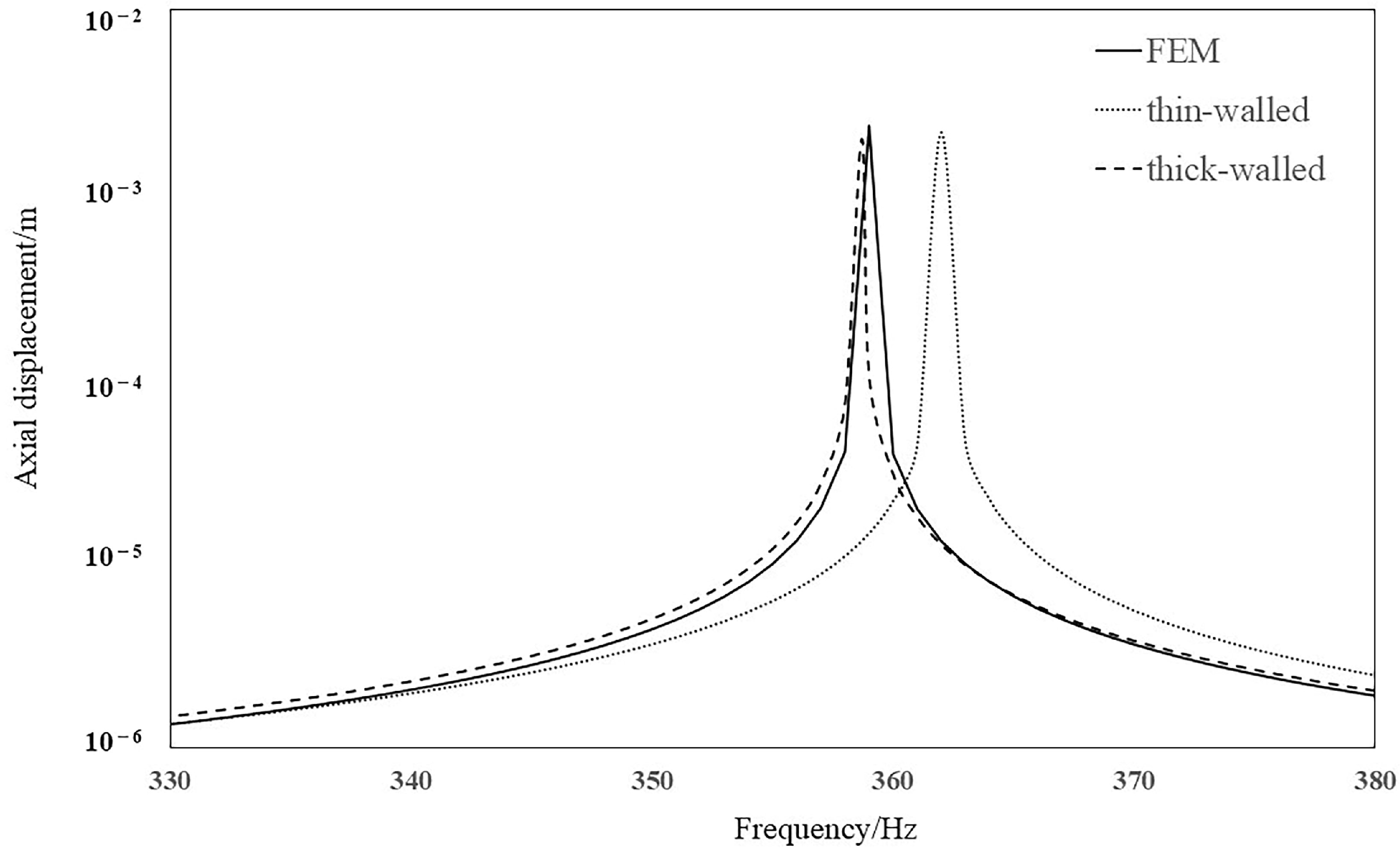
3.1. Validation of the Current Calculation Method

In order to validate the accuracy of the above calculation procedure, numerical examples from the literature [20] were carried out. The natural frequencies of a straight pipe are calculated in

Table 1. Natural frequencies in comparison with the literature results.

Axial (Hz) [20]	173	289	459	485	636	750	918	968
Axial (present) (Hz)	169	282	451	470	621	734	898	941
Error (%)	−2.31%	−2.42%	−1.74%	−3.09%	−2.36%	−2.13%	−2.18%	−2.79%
Transverse (Hz) [20]	13	36	70	116	173	241	320	411
Transverse (present) (Hz)	13	37	73	121	179	247	327	417
Error (%)	0%	2.8%	4.3%	4.3%	3.5%	2.5%	2.1%	1.5%

. The material properties are length L = 4.502 m, radius R = 26.01 mm, thickness e = 3.945 mm, Young’s modulus E = 168 GPa, pipe density ${\rho }_{\mathrm{p}}$ = 7985 kg/m³, Poisson’s ratio $\mu$ = 0.29, section area of fluid $A_{\mathrm{f}}$ = 2125 mm², and section area of pipe $A_{\mathrm{p}}$ = 694 mm². The internal fluid is water with a bulk modulus of 2.14 GPa and with a density ${\rho }_{\mathrm{p}}$ = 999 kg/m³. The ends of the pipe are free. The mass of the plugs in the ends are m₁ = 1.312 kg and m₂ = 0.3258 kg. It can be seen in Table 1 that the results using the present theory are in agreement with those from the experiment in the literature, which validates the effectiveness of the present theory.

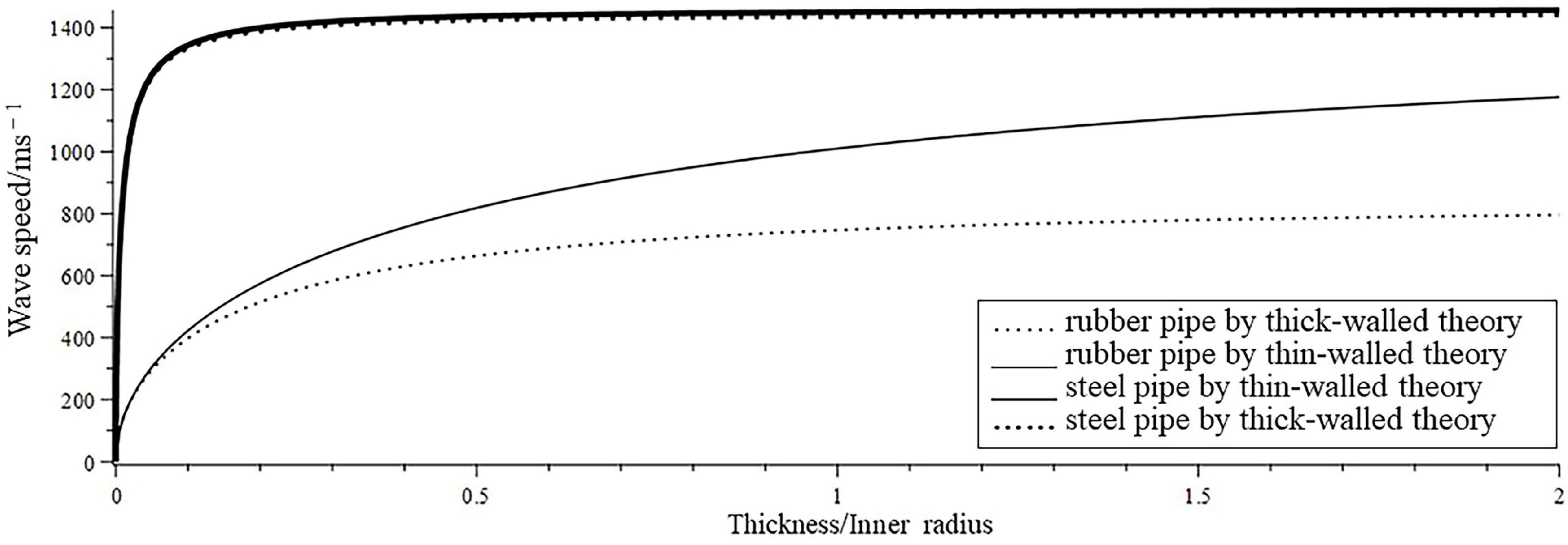
3.2. The Applicability Analysis of the Thick-Walled Theory and the Thin-Walled Theory

The fluid pressure wave velocity in the axial vibration is $c_{\mathrm{f}}=\sqrt{\frac{K^{*}}{{\rho }_{\mathrm{f}}}}$. In the present thick-walled theory, $K^{*}={\left(\frac{1}{K}+\frac{2}{E}\left[\frac{R}{e}\left(1-\frac{{\mu }^2}{1+\frac{e}{2R}}\right)+\frac{1+\frac{e}{R}}{2+\frac{e}{R}}+\mu \right]\right)}^{-1}$, while in the traditional thin-walled theory, $K^{*}={\left(\frac{1}{K}+\frac{2}{E}\frac{R}{e}\left(1-{\mu }^2\right)\right)}^{-1}$ [20]. Therefore, in order to analyze the applicability of these two theories, several numerical examples were carried out, as described in this section.

First, the FEM software Abaqus 6.14 was used to calculate the FSI vibration of a pipe. Solid elements were used to model the pipe structure in Abaqus. The straight pipe has the length of 1 m, and the thickness and inner radius are both 0.05 m. The other material properties remained the same as in Section 3.1. A harmonic axial excitation was applied on one end, and the corresponding displacement response is shown in Figure 4.

In Abaqus, the pipe was modeled by solid elements and the internal fluid was modeled by acoustic solid elements (element type AC3D8). The pipe wall and internal fluid were coupled through a Tie connection. The fluid displacement and the axial displacement of the pipeline are consistent. In order to derive stable and accurate results, 117,800 elements are used to establish the model in Abaqus, which demands 3 h for calculating vibration responses in frequency domain 0–1000 Hz. By using the present SEM to calculate the same model, only one element is necessary. Related thick-walled and thin-walled programs were completed and calculated in Maple 2019. It only takes 5 min to derive the final results. Apparently, SEM has great advantages in calculating efficiency and accuracy. Figure 4 shows that the thick-walled theory is more adequate in this numerical example, since the ratio of thickness and radius reaches 1, which indicates that the axial stress should not be ignored for thick-walled pipes.

The flexible pipe was considered afterwards. The axial wave speeds of a metal pipe/a rubber pipe (with Young’s modulus 3 GPa, Poisson’s ratio 0.48, and density 1200 kg/m³) were calculated by both the thick-walled theory and the thin-walled theory. The results are shown in Figure 5. When the ratio of the thickness and inner radius of the rubber pipe reaches 0.1, the wave speeds may have great differences. As the ratio becomes larger, the differences are larger. The two theories for metal pipes almost remain consistent. Only when the ratio of the thickness and radius reaches 0.5 do differences begin to appear.

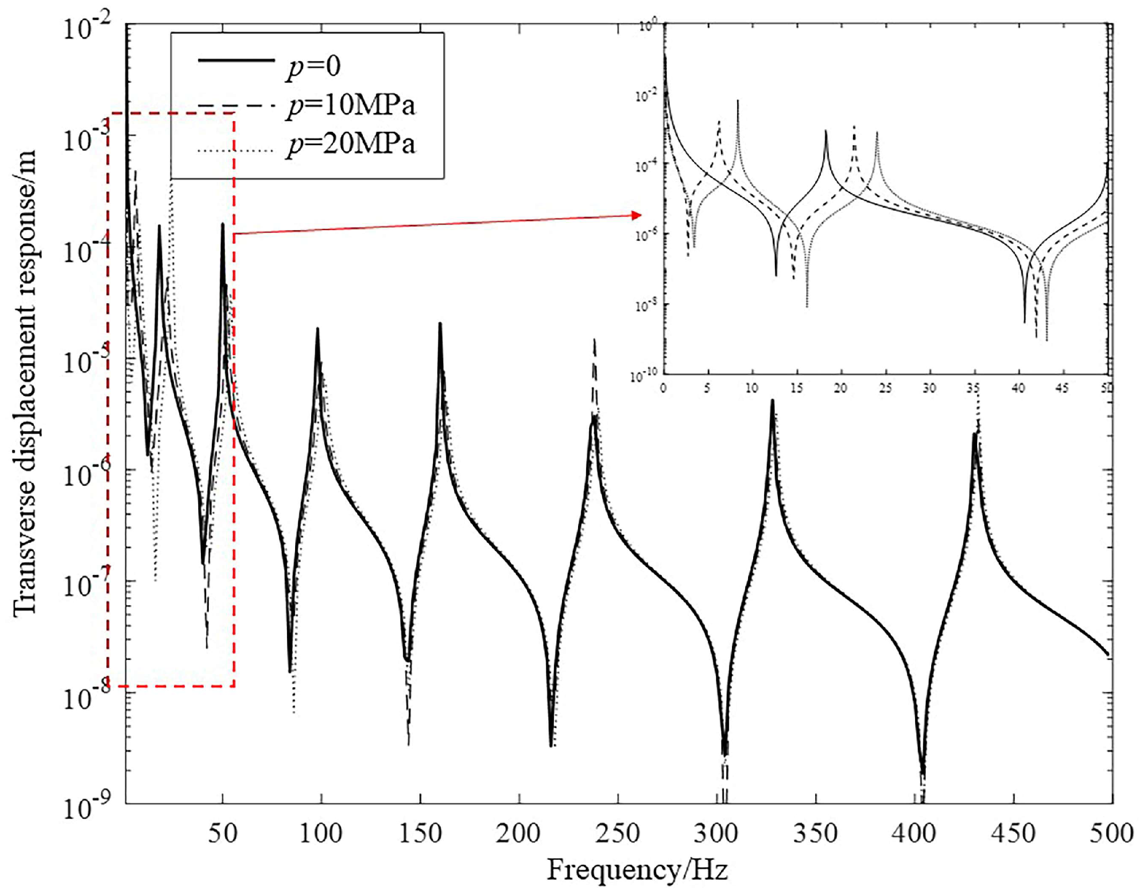
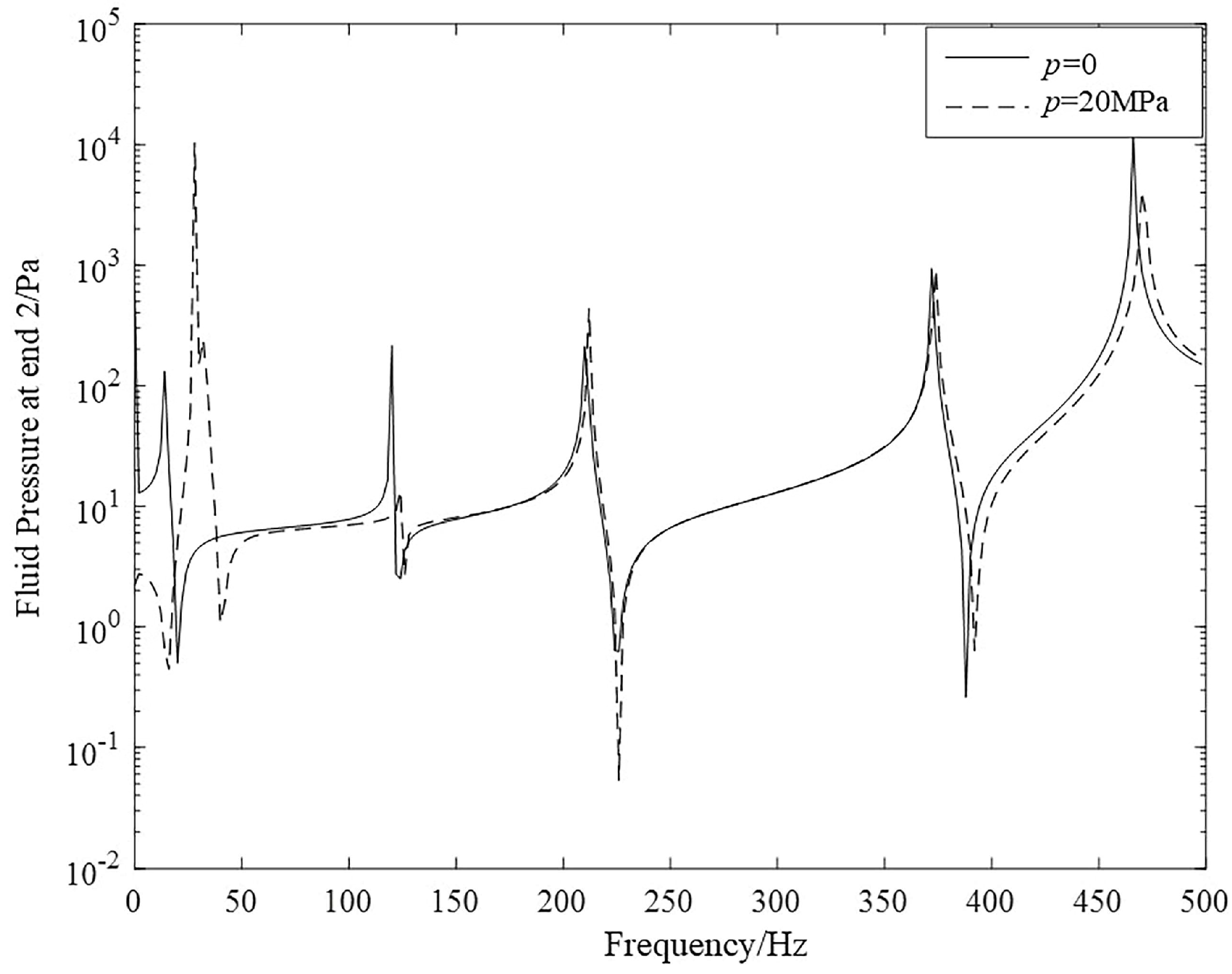
3.3. The Influences of Internal Hydrostatic Pressure under Harmonic Excitation

The transverse unit harmonic excitation was applied on a steel straight pipe, and the transverse and axial displacement responses were calculated, as shown in Figure 6 and Figure 7. The length of the pipe was 5 m, and plugs were used in both ends. The internal fluid was water. The inner radius of the pipe was 40 mm, and the thickness was 5 mm.

In the lower frequency domain, especially 0–50 Hz, the influences of hydrostatic pressure were rarely larger than those in the higher frequency domain. It is apparent in Figure 7 that some resonance peaks are in perfect coincidence since these peaks arise via axial modes and FSI modes. Other peaks arise via transverse modes, as shown in Figure 6. Therefore, the hydrostatic pressure mainly affects the transverse vibration.

The natural frequencies in the lower frequency domain of a straight steel water-filled pipe with a length of 2 m under different thicknesses and internal hydrostatic pressures are shown in

Table 2. Natural frequencies of straight pipelines with different thicknesses and internal pressures.

R (mm)	t (mm)	t/R	Pressure	Natural Frequencies (Hz)
40	5	0.125	p = 20 MPa	8	24	54	101	153	165
			p = 10 MPa	6	21	52	99	154	162
			p = 0	-	-	50	98	155	160
40	8	0.2	p = 20 MPa	7	24	59	111	166	180
			p = 10 MPa	5	23	57	110	166	179
			p = 0	-	21	56	109	166	178
40	10	0.25	p = 20 MPa	7	25	61	116	163	188
			p = 10 MPa	5	23	60	115	163	187
			p = 0	-	22	59	114	163	187
40	12	0.3	p = 20 MPa	6	25	63	120	160	196
			p = 10 MPa	-	24	62	120	160	195
			p = 0	-	23	61	119	160	194
40	15	0.375	p = 20 MPa	6	26	66	126	157	206
			p = 10 MPa	4	25	65	126	157	205
			p = 0	-	24	65	125	157	205
40	20	0.5	p = 20 MPa	5	27	71	136	154	221
			p = 10 MPa	-	26	70	135	154	221
			p = 0	-	26	70	135	154	221

. The ends of the pipeline were free but filled with plugs. The first six natural frequencies are listed in Table 2. The internal pressure increases the natural frequencies but has little effect on the fifth natural frequency, which is the axial mode. It is noticed that the influence of the pressure becomes smaller with increasing thickness, especially for relatively higher frequencies.

We consider a short rubber pipe (with length of 0.1 m) used to connect two steel pipes (with a length of 1 m). Suppose the internal hydrostatic pressure of the assembled pipeline is 20 MPa. When one end is subjected to a transverse harmonic excitation, the magnitude and duration are 80 kN and 2 ms, respectively. The vibration transmission characteristics at the end of the assembled pipeline are calculated by the following:

$$L_v=10\lg \left({\displaystyle \sum _{i=1}^n{10}^{L_{vi}/10}}\right)\mathrm{where}, L_{vi}=20\lg \frac{v}{v_0}\left(v_0={10}^{-5} \mathrm{m}/\mathrm{s}\right),$$

where n represents all the frequency points (0–1000 Hz).

The transverse vibration acceleration levels are calculated in

Table 3. Vibration acceleration level at the end of the assembled pipeline.

R (mm)	t (mm)	t/R	Steel–Rubber–Steel (dB)	Steel (dB)
40	5	0.125	213.14	216.60
40	8	0.2	211.97	214.00
40	10	0.25	210.82	212.40
40	12	0.3	209.75	215.16
40	15	0.375	211.09	209.27
40	20	0.5	206.24	208.78

. Apparently, relatively thin-walled pipelines have higher vibration acceleration levels. The internal pressure increases the rigidity of the pipeline, while the introduction of a flexible pipe would reduce the rigidity of the assembled pipeline, which is evident for cases of t/R ≤ 0.3. As for relatively thick pipes, the cross-sectional area is larger, and the introduction of a flexible pipe has less effect on the vibration transmission.

A two-dimensional L-type pipe is shown in Figure 8. The elbow pipe can be assembled with several straight pipe elements. The material properties are L = 900 mm, R = 127 mm, a = 45 mm, e = 4.5 mm, E = 210 (1 + 0.001i) GPa, μ = 0.3, and ρ = 7900 kg/m³. The last straight pipe was assembled using a rubber pipe with a length of 0.1 m and a steel pipe with a length of 0.8 m. The ends of the pipeline were free, and plugs were used. An axial unit harmonic excitation was applied on the left end, and the vibration velocity and sound pressure responses are shown in Figure 9 and Figure 10, respectively.

As shown in the figures, the hydrostatic pressure mainly affects the vibration characteristics in the lower frequency domain. The inner pressure may increase the rigidness of the flexible pipe, which leads to the increase in low-order modes. Such effects may increase the vibration transmission.

The overall sound pressure level is as follows:

$$L_p=10\lg \left({\displaystyle \sum _{i=1}^n{10}^{L_{pi}/10}}\right)\mathrm{where}, L_{pi}=20\lg \frac{p}{p_0}\left(p_0=2\times {10}^{-5 }\mathrm{Pa}\right),$$

where n represents all the frequency points (0–500 Hz).

The comparison of the pressure level and velocity level are shown in

Table 4. The overall sound pressure level and overall vibration velocity level of different pipe types.

Pipe Type	Inner Pressure	Overall Vibration Velocity Level (dB)	Overall Sound Pressure Level (dB)
Including rubber pipe	p = 0	152.6	175.7
	p = 20 MPa	160.3	175.4
Pure metal pipe	p = 0	155.4	176.4
	p = 20 MPa	171.6	174.2

. The internal hydrostatic pressure apparently increases the overall vibration velocity level but has almost no effects on the overall sound pressure level. This also indicates that the internal pressure mainly affects the transverse vibration transmission but has no effect on the axial sound transmission. In addition, when subjected to inner pressure, the assembled pipes, including the rubber pipe, are more suitable for vibration and sound control.

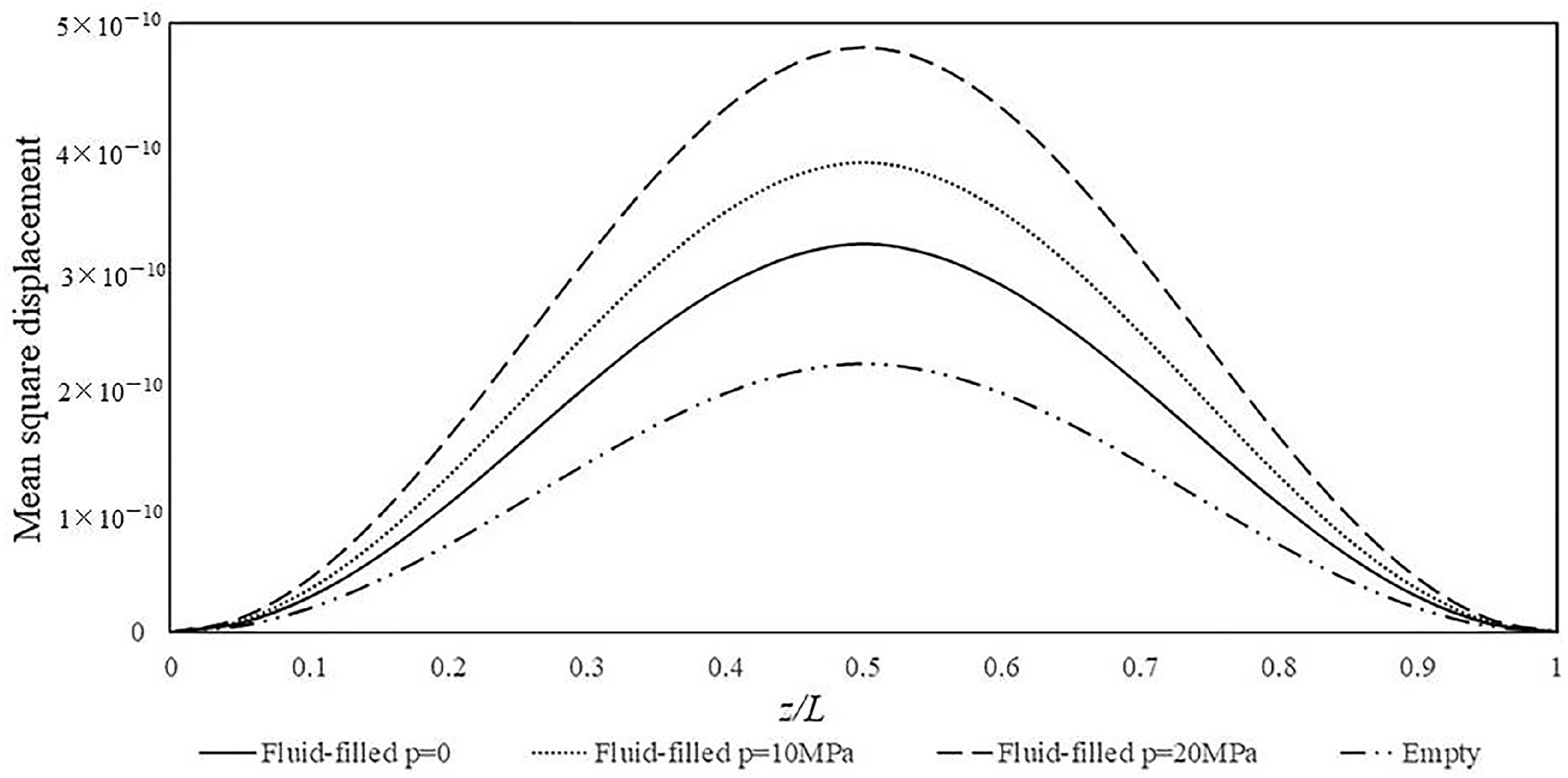
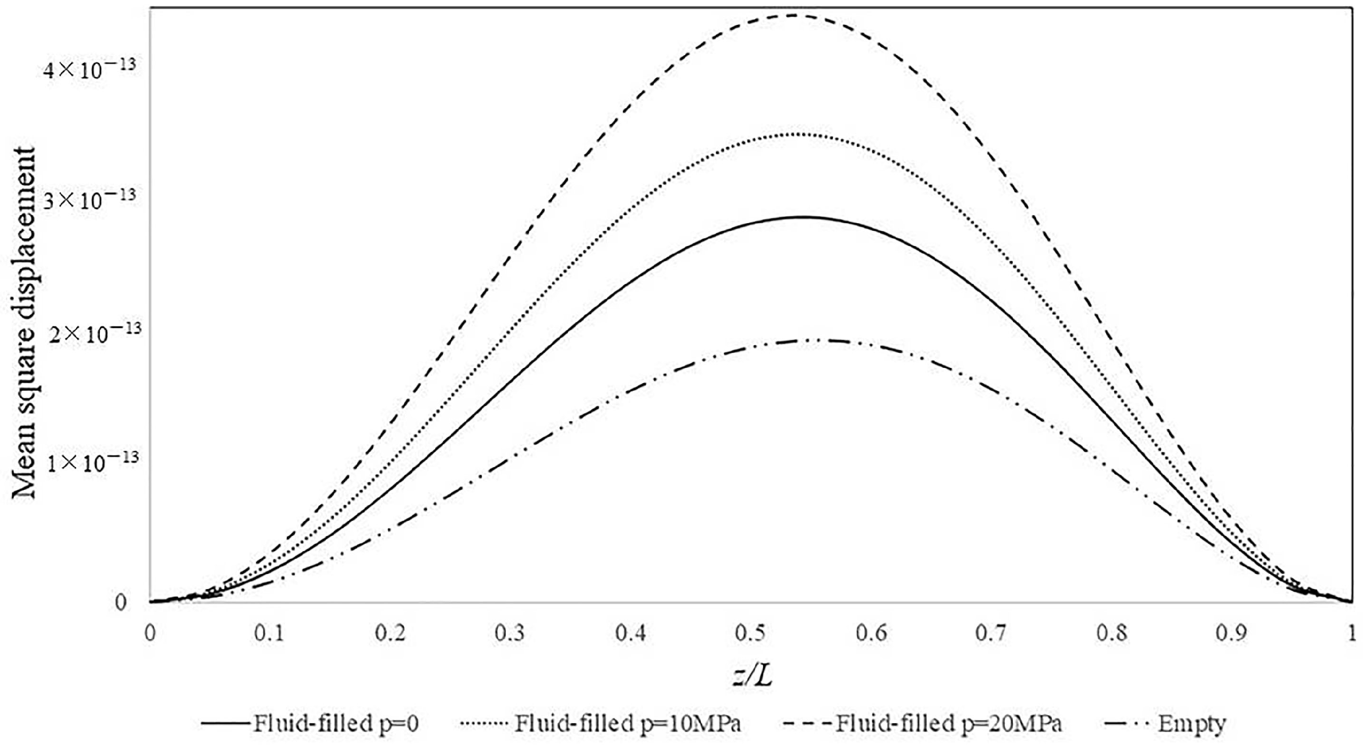
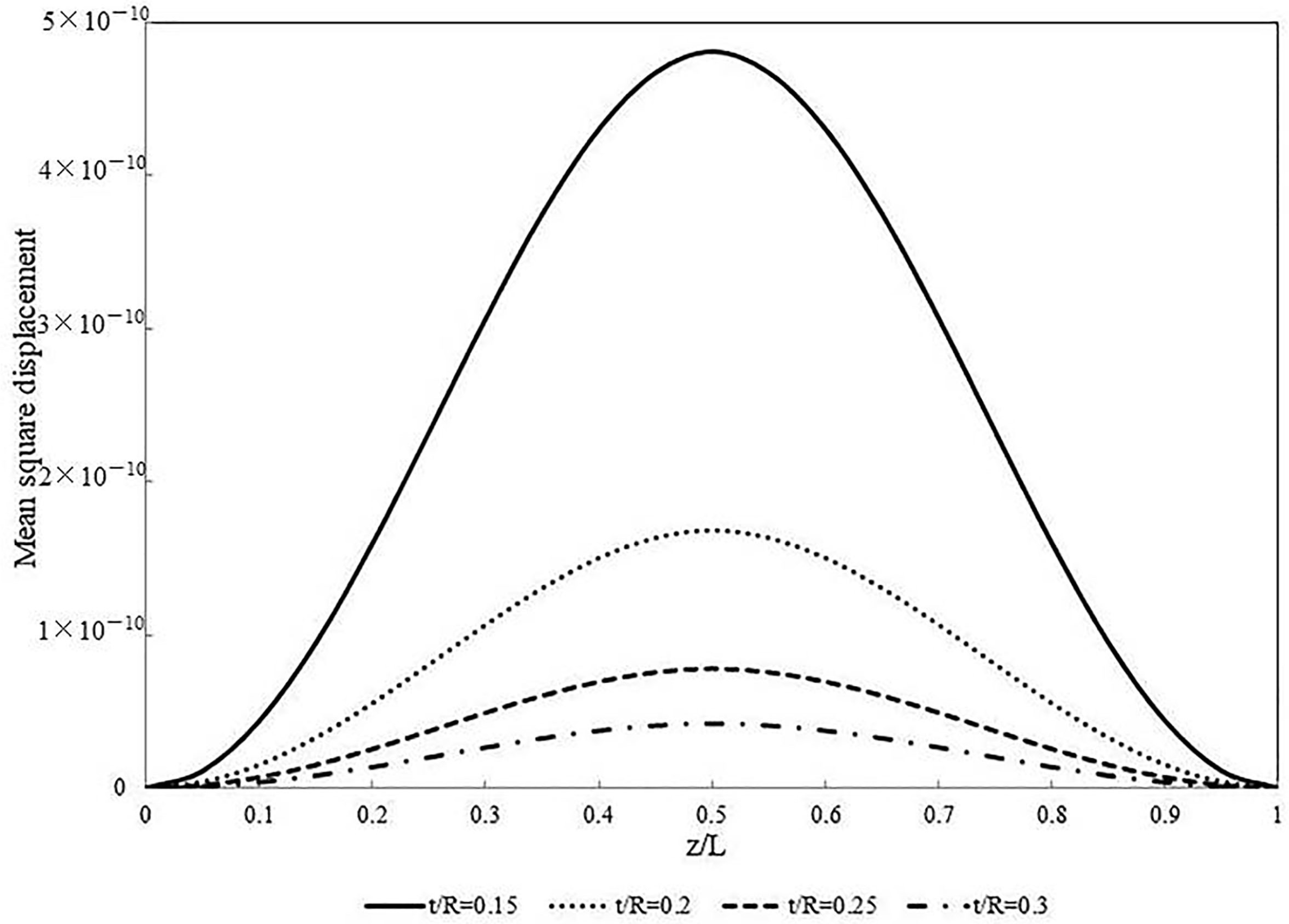
3.4. The Influences of Internal Hydrostatic Pressure under Random Loads

A simply supported fluid-filled pipe with internal pressure was considered in this example. The material properties are the same as those in Section 3.1. The pipeline was subjected to ideal white noise excitation, either concentrated at the midpoint or uniformly distributed along the length. The input cross-spectral density, S_ff and S_θ, are considered to be constants. The mean square displacement at any point can be obtained by integrating the cross-spectral density over the entire frequency range, given as follows:

$$〈ww〉={\displaystyle {\int }_0^{\infty }{S}_w\left(z,\omega \right)}\mathrm{d}\omega .$$

The calculated frequency range was 0–100 Hz. Figure 11 and Figure 12 show the mean square displacements along the pipeline for the concentrated case and distributed case, respectively. Suppose that the inner radius (R = 26.01 mm) and internal hydrostatic pressure (p = 20 MPa) remain the same; Figure 13 and Figure 14 show the mean square displacement along the pipeline with different thicknesses.

It is noted that with increasing internal hydrostatic pressure, the mean square displacements also increase. The mean square displacement evidently decreases with increasing t/R, which indicates that relatively thick-walled pipes are more suitable for withstanding internal pressure and random loads. Meanwhile, the displacements under concentrated loads are higher than those under distributed loads.

4. Conclusions

The FSI equations for fluid-filled, thick-walled pipelines with internal hydrostatic pressure were derived in this paper. The spectral element method and pseudo-excitation method were applied to solve the vibration responses to harmonic excitations and random loads. The present method was validated with a comparison with the previous literature data and an FEM calculation. The present thick-walled theory was compared with the traditional thin-walled theory. The effects of the hydrostatic pressure were investigated afterwards. The results show the following:

(1)

The axial wave speeds are different in the thick-walled theory and thin-walled theory. With an increase in the ratio of the thickness and radius, the differences also increase, especially for flexible pipes.

(2)

The internal hydrostatic pressure mainly affects the transverse vibration but has little effect on axial vibration transmissions.

(3)

The transverse natural frequencies become larger with increasing internal pressure. Such influences are especially significant in the lower frequency domain.

(4)

The downstream overall vibration velocity level increases due to the existence of internal pressure, which indicates that the hydrostatic pressure would increase the vibration transmission. Introducing flexible pipes may improve this condition.

(5)

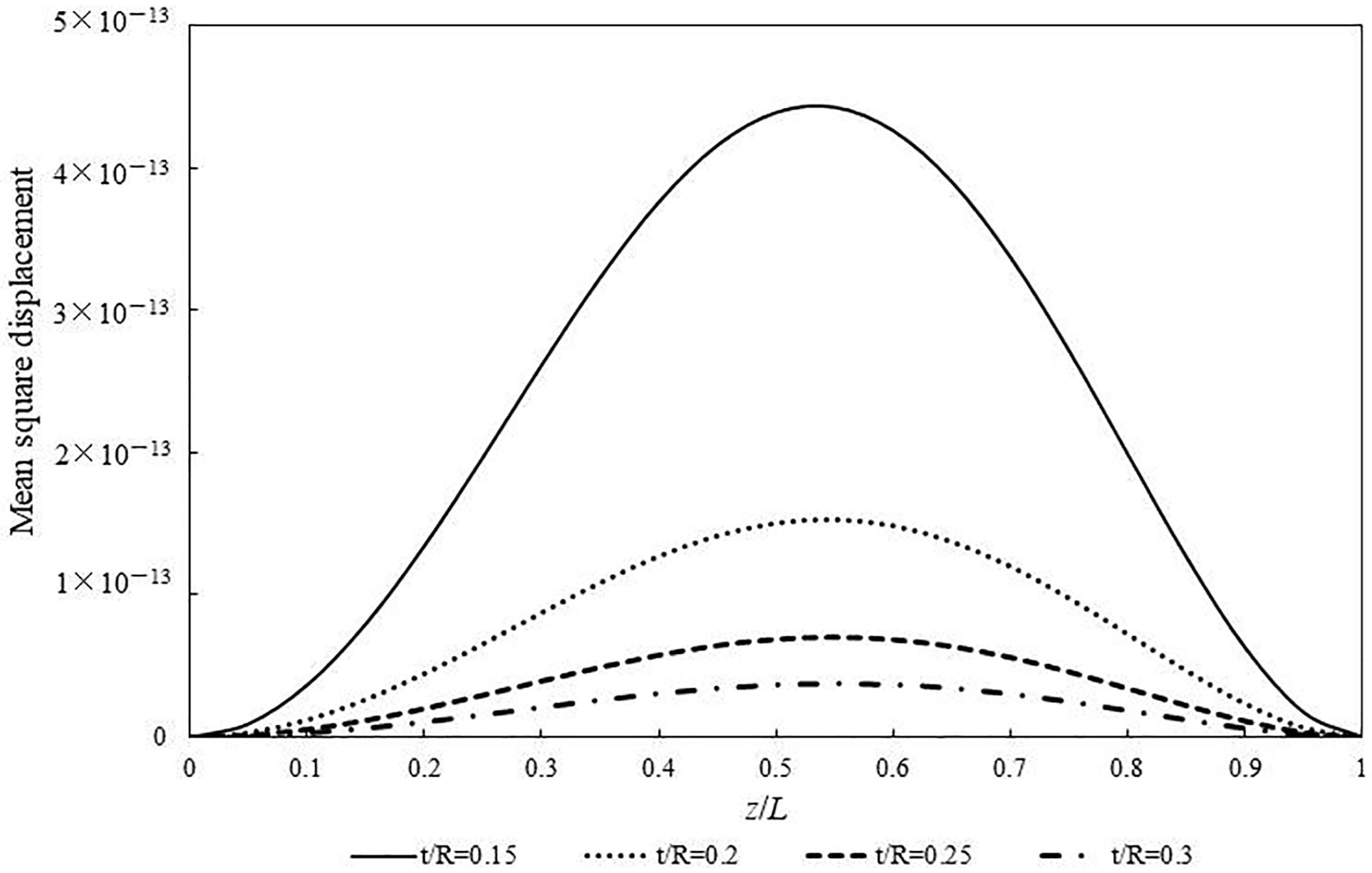
The internal pressure also increases the mean square displacement along the pipeline when subjected to random loads. Relatively smaller displacements are presented by relatively thick-walled pipelines or under distributed random loads, as expected.

The present work may provide a reference for the design of pressurized fluid-filled pipelines. Further research could be carried out on the optimization of the pipeline structure and pipeline material for the purpose of vibration control.

References

1. Jiang, X.L. On the ship pipeline system. Sci. Technol. Vision 2012, 25, 211–301. [Google Scholar]
2. Wei, Z.D.; Li, B.R.; Du, J.M. Theoretical and experimental investigation of flexural vibration transfer properties of high-pressure periodic pipe. Chin. Phys. Lett. 2016, 33, 141. [Google Scholar] [CrossRef]
3. Huang, P. Study on Hydroelastic Instability and Random Response Analysis of Tube Arrays. Ph.D. Thesis, Tsinghua University, Beijing, China, 2006. [Google Scholar]
4. Fung, Y.C.; Kaplan, A.; Sechler, E.E. On the vibration of thin cylindrical shells under internal pressure. J. Aeronaut. Sci. 1957, 24, 650–660. [Google Scholar] [CrossRef]
5. Miserentino, R.; Vosteen, L.F. Vibration Tests of Pressurized Thin-Walled Cylindrical Shells; TND-3066; National Aeronautics and Space Administration: Washington, DC, USA, 1965. [Google Scholar]
6. Keltie, R.F. The effect of hydrostatic pressure fields on the structural and acoustic response of cylindrical shells. J. Acoust. Soc. Am. 1986, 79, 595–603. [Google Scholar] [CrossRef]
7. Xie, G. Influence of hydrostatic pressure on sound radiation of cylindrical shell with ring ribs. J. Wuhan Univ. Technol. 1995, 1, 77–79. [Google Scholar]
8. Zhang, Y.L.; Gorman, D.G.; Reese, J.M. Vibration of prestressed thin cylindrical shells conveying fluid. Thin-Walled Struct. 2003, 41, 1103–1127. [Google Scholar] [CrossRef]
9. Liu, Z.; Li, T.; Liu, J. Analysis of dispersion characteristics of liquid-filled cylindrical shells considering hydrostatic pressure. Ship Mech. 2009, 13, 635–640. [Google Scholar]
10. Iakovlev, S.; Dooley, G.; Williston, K.; Gaudet, J. Evolution of the reflection and focusing patterns and stress states in two-fluid cylindrical shell systems subjected to an external shock wave. J. Sound Vib. 2011, 330, 6254–6276. [Google Scholar] [CrossRef]
11. Chen, L.; Li, L.; Zhang, Y. Analysis of acoustic radiation characteristics of cylindrical shell structures with local prestress. J. Shanghai Jiaotong Univ. 2014, 48, 1084–1089. [Google Scholar]
12. Gao, H.; Shuai, C.; Ma, J.; Xu, G. Free Vibration of Rubber Matrix Cord-Reinforced Combined Shells of Revolution Under Hydrostatic Pressure. J. Vib. Acoust. Trans. ASME 2022, 144, 011002. [Google Scholar] [CrossRef]
13. Hua, G.; Sang, C.; Ma, J.; Cheng, Y. Vibro-acoustic characteristics of rubber matrix cord-reinforced combined shells of revolution under hydrostatic pressure. Appl. Acoust. 2022, 190, 108642. [Google Scholar] [CrossRef]
14. Neto, H.R.; Cavalini, J.A.; Vedovoto, J.M.; Neto, A.S.; Rade, D.A. Influence of seabed proximity on the vibration responses of a pipeline accounting for fluid-structure interaction. Mech. Syst. Signal Pr. 2019, 114, 224–238. [Google Scholar] [CrossRef]
15. Kiryukhin, A.V.; Mil’man, O.O.; Ptakhin, A.V.; Serezhkin, L.N.; Isaev, S.A. Investigation of Pressure Pulsations and Power Loads in the Compensator with the Aim of Reducing Vibration Transfer in a Pipeline with a Liquid. J. Eng. Phys. Thermophys. 2019, 92, 1517–1523. [Google Scholar] [CrossRef]
16. Yamilev, M.Z.; Masagutov, A.M.; Nikolaev, A.K.; Pshenin, V.V.; Zaripova, N.A.; Plotnikova, K.I. Modified equations for hydraulic calculation of thermally insulated oil pipelines for the case of a power-law fluid. Nauka Tehnol. Trubopr. 2021, 11, 388–395. [Google Scholar]
17. Korshak, A.A.; Pshenin, V.V. Modeling of water slug removal from oil pipelines by methods of computational fluid dynamics. Neft. Khozyaystvo-Oil Ind. 2023, 10, 117–122. [Google Scholar] [CrossRef]
18. Cao, Y.; Ma, H.; Guo, X.; Ge, H.; Li, H.; Lin, J. Experimental Study on Pressure Pulsation and Acceleration Response of Fluid Conveying Pipeline Under Multi-Excitation. ASME J. Press. Vessel Technol. 2023, 145, 051401. [Google Scholar] [CrossRef]
19. Wiggert, D.C.; Hatfield, F.J.; Stuckenbruck, S. Analysis of Liquid and Structural Transients in Piping by the Method of Characteristics. ASME J. Fluids Eng. 1987, 109, 161–165. [Google Scholar] [CrossRef]
20. Zhang, L.; Tijsseling, A.S.; Vardy, A.E. FSI analysis of liquid-filled pipes. J. Sound Vib. 1999, 224, 69–99. [Google Scholar] [CrossRef]
21. Lesmez, M.W. Modal Analysis of Vibrations in Liquid-Filled Piping Systems. Ph.D. Thesis, Michigan State University, East Lancing, MI, USA, 1989. [Google Scholar]
22. Tentarelli, S.C. Propagation of Noise and Vibration in Complex Hydraulic Tubing Systems. Ph.D. Thesis, Lehigh University, Bethlehem, PA, USA, 1990. [Google Scholar]
23. Caf, J.D. Analysis of Pulsations and Vibrations in Fluid-Filled Pipe Systems. Ph.D. Thesis, Eindhoven University of Technology, Eindhoven, The Netherlands, 1994. [Google Scholar]
24. Zhang, Z.Y. Study on Vibration Characteristics and Energy Flow in Fluid-Filled Pipe Systems Considering Fluid-Structure Interaction. Ph.D. Thesis, Shanghai Jiao Tong University, Shanghai, China, 2000. [Google Scholar]
25. Li, Y.H. Study on Vibration, Noise, and Characteristics of Fluid-Structure Coupled Pipe Systems. Ph.D. Thesis, Harbin Engineering University, Harbin, China, 2011. [Google Scholar]
26. Everstine, G.C. Dynamic analysis of fluid-filled piping systems using finite element techniques. J. Press. Vessel.-Technol. ASME 1986, 108, 57–61. [Google Scholar] [CrossRef]
27. Hansson, P.A.; Sandberg, G. Dynamic finite element analysis of fluid-filled pipes. Comput. Methods Appl. Mech. Eng. 2001, 190, 3111–3120. [Google Scholar] [CrossRef]
28. Lee, U.; Kim, J. Dynamics of branched pipeline systems conveying internal unsteady flow. Trans. ASME 1999, 121, 114–122. [Google Scholar] [CrossRef]
29. Sandvik, A.; Østby, E.; Thaulow, C. A probabilistic fracture mechanics model including 3D ductile tearing of bi-axially loaded pipes with surface cracks. Eng. Fract. Mech. 2008, 75, 76–96. [Google Scholar] [CrossRef]
30. Kainat, M.; Lin, M.; Roger Cheng, J.J.; Martens, M.; Adeeb, S. Effects of the initial geometric imperfections on the buckling behavior of high-strength uoe manufactured steel pipes. J. Press. Vessel. Technol. 2016, 138, 051206. [Google Scholar] [CrossRef]
31. Franci, A. Lagrangian finite element method with nodal integration for fluid–solid interaction. Comput. Part Mech. 2020, 8, 389–405. [Google Scholar] [CrossRef]
32. Shahzamanian, M.M.; Lin, M.; Kainat, M.; Yoosef-Ghodsi, N.; Adeeb, S. Systematic literature review of the application of extended finite element method in failure prediction of pipelines. J. Pipeline Sci. Eng. 2021, 1, 241–251. [Google Scholar] [CrossRef]
33. Hicham, F.; Abdelhamid, H.; Nabil Mohammed, O. Fluid-structure interactions of internal pressure pipeline using the hierarchical finite element method. Adv. Mech. Eng. 2021, 13, 16878140211041262. [Google Scholar] [CrossRef]
34. Wu, G.X.; Zhao, X.L.; Shi, D.D.; Wu, X. Analysis of Fluid-Structure Coupling Vibration Mechanism for Subsea Tree Pipeline Combined with Fluent and Ansys Workbench. Water 2021, 13, 955. [Google Scholar] [CrossRef]
35. Yu, T.; Zhang, Z.; Zhang, D.; Juan, M.; Jin, J. Vibration Analysis of Multi-Branch Hydraulic Pipeline System Considering Fluid—Structure Interaction. Appl. Sci. 2022, 12, 12902. [Google Scholar] [CrossRef]
36. Zhu, H.Z.; Wang, W.B.; Yin, X.W.; Gao, C.F. Spectral element method for vibration analysis of three-dimensional pipes conveying fluid. Int. J. Mech. Mater. Des. 2019, 15, 345–360. [Google Scholar] [CrossRef]
37. Wu, J.H.; Tijsseling, A.S.; Sun, Y.D. Vibration analysis by impedance synthesis method of three-dimensional piping connected to a large circular cylindrical shell. Mech. Syst. Signal Process. 2023, 188, 110063. [Google Scholar] [CrossRef]
38. Wu, J.H.; Sun, Y.D. An exact solution for vibration analysis of pipe coupled with conical-ring stiffened cylindrical shells with arbitrary boundary condition. Ocean Eng. 2022, 266, 112861. [Google Scholar] [CrossRef]
39. Lin, J.H.; Zhang, Y.H. The pseudo-excitation method and its industrial applications in China and abroad. Appl. Math. Mech. 2017, 38, 1–31. [Google Scholar]
40. Lin, J.H.; Zhang, W.S.; Williams, F.W. Pseudo-excitation algorithm for non-stationary random seismic responses. Eng. Struct. 1992, 44, 683–687. [Google Scholar]
41. Tijsseling, A.S. Water hammer with fluid-structure interaction in thick-walled pipes. Comput. Struct. 2007, 85, 844–851. [Google Scholar] [CrossRef]
42. Xu, Z.L. Elasticity, 5th ed.; Higher Education Press: Beijing, China, 2016. [Google Scholar]
43. Liang, Z.; Zhang, J.; Zhang, H. Submarine Pipeline Mechanics; Science Press: Beijing, China, 2018; pp. 38–40. [Google Scholar]
Figure 1. Forces on the infinitesimal segment of a pipeline.
Jmse 11 02338 g001
Figure 2. Forces on an infinitesimal segment of fluid.
Jmse 11 02338 g002
Figure 3. Nodal displacements and nodal forces on the pipe element.
Jmse 11 02338 g003
Figure 4. The axial displacement response calculated by thick-walled theory/thin-walled theory/FEM.
Jmse 11 02338 g004
Figure 5. The fluid pressure wave speed of different pipes using the thick-walled theory or thin-walled theory.
Jmse 11 02338 g005
Figure 6. The transverse displacement response of the pipe end under different hydrostatic pressures.
Jmse 11 02338 g006
Figure 7. The axial displacement response of the pipe end under different hydrostatic pressures.
Jmse 11 02338 g007
Figure 8. The L-type pipeline.
Jmse 11 02338 g008
Figure 9. The vibration velocity response in the x direction.
Jmse 11 02338 g009
Figure 10. The fluid pressure response on the upper end of the pipeline.
Jmse 11 02338 g010
Figure 11. Mean square displacement along the pipeline under a concentrated random load.
Jmse 11 02338 g011
Figure 12. Mean square displacement along the pipeline under a distributed random load.
Jmse 11 02338 g012
Figure 13. Mean square displacement along the pipeline with different thicknesses under a concentrated random load.
Jmse 11 02338 g013
Figure 14. Mean square displacement along the pipeline with different thicknesses under a distributed random load.
Jmse 11 02338 g014