Anti-Disturbance Lyapunov-Based Model Predictive Control for Trajectory Tracking of Dynamically Positioned Ships

Abstract

Trajectory tracking is a fundamental task of the dynamic positioning (DP) system. This paper studies the problem of trajectory tracking of DP ships constrained by control inputs under environmental disturbances. To solve this problem, we develop a novel anti-disturbance Lyapunov-based model predictive control (ADLMPC) scheme. Firstly, an extended state observer (ESO) is designed to estimate environmental disturbances. By combining the ESO with Lyapunov-based model predictive control, the ADLMPC scheme is devised. Secondly, a virtual controller which satisfies input constraints is developed by backstepping and the auxiliary dynamic system, and it is integrated into the Lyapunov contraction constraint in ADLMPC. We show that if the parameters for the virtual controller are appropriately determined, the recursive feasibility of ADLMPC is theoretically guaranteed, and the uniform ultimate boundedness of all signals in the trajectory tracking control system is achieved. Finally, the simulation results display the efficacy and superiorities of the ADLMPC scheme.

1. Introduction

The dynamic positioning (DP) system can control a ship to keep it in the desired position or navigate on a pre-determined track by using thrusters actively and automatically to balance the environmental forces caused by wind, waves, current, etc. The DP technique has been widely applied in many marine engineering industries, such as offshore drilling and deep water pipe laying [1].

Trajectory tracking is an essential task for DP ships. Typical trajectory tracking tasks for DP ships including oceanic exploration, area target searching, pipe laying, etc.; some of these tasks require a high precision in tracking performance. Therefore, the design of a high-level DP controller with high performance is crucial. However, as the ship is a nonlinear, strongly coupled, and constrained system, it brings severe challenges to the design of the controller. Moreover, the DP ship is frequently perturbed by unknown environmental disturbances, and anti-disturbance should be solved. Various control theories have been resorted to for trajectory tracking problems by plenty of researchers. A nonlinear trajectory tracking controller was designed by backstepping in [2]; this method can avoid the linearization of the model of the ship. The dynamic surface control technique, which can prevent “computation explosion” in backstepping design, was applied in the controller [3]. This controller successfully made the underactuated ship track a smooth curve trajectory. However, this technique requires high accuracy in the controlled model. Under unknown environmental disturbances and model uncertainties, the sliding mode control was adopted in the ship trajectory tracking controller due to its robustness [4,5]. The sliding mode control theory combined with the control allocation algorithm was adopted in an AUV to complete the task of trajectory tracking and station-keeping [4,5]. The simulation results and experimental results in [4,5] verified the tracking and station-keeping performance and the system robustness under the effects of unknown disturbances. However, the “chattering” effect in sliding mode control cannot be entirely eliminated. Observers were introduced to the control system to estimate unknown disturbances and model uncertainties in [6,7,8,9]. The estimated values were utilized to design the trajectory tracking controller such that the ship could overcome the influence of disturbances and uncertainties. Corresponding simulations showed that the trajectory tracking accuracy was improved. Besides the trajectory tracking of ships, the strategy of the controller combined with the observer is also applied in many other fields. In [10], a fast terminal sliding mode control technique based on the disturbance observer is developed to stabilize the underactuated robotic system. Both simulation results and experimental validations on a cart-inverted pendulum system were provided to demonstrate the effectiveness of the proposed method. A lumped perturbation observer-based extended multiple sliding surface control method was presented for the SISO system with matched and unmatched uncertainties, and numerical simulation was performed to verify the efficacy of the proposed method compared with integral type sliding mode control and dynamic surface control [11]. With the development of intelligent control theories, fuzzy control, adaptive control, neural network, etc., they were combined with other advanced control theories to achieve ship trajectory tracking [12,13,14]. In [15], an adaptive non-singular fast terminal sliding mode control with an integral surface for the tracking control of nonlinear systems with external disturbances was developed. The disturbances were compensated for by an appropriate parameter-tuning adaptation law, and the tracking task was accomplished by a new fast terminal sliding scheme with a self-tuning algorithm to guarantee control inputs were chattering-free. Integrating these different theories can overcome each other’s drawbacks and improve control performance, but the design of such controllers is relatively complicated. Input constraints are not considered in most of the above controllers, which may deteriorate control performance and even the stability of the system in practical applications. In fact, some techniques can solve the problem of control input constraints, such as the composite nonlinear feedback (CNF) method. A CNF controller was developed to achieve the reference tracking of uncertain time-delayed linear systems constrained by actuator saturation. The simulation results illustrated that the transient performance was improved [16]. However, the CNF method has not been fully developed for nonlinear systems.

Compared with other control techniques, the distinct advantage of Model Predictive Control (MPC) is its capability to cope with system constraints explicitly and optimize control performance, so it is widely applied in various industries [17]. However, stability cannot be guaranteed due to the optimal control problem with a finite horizon [18]. According to recent research, there are two main ways to achieve stability. The first is constructing the appropriate terminal cost and constraint set for the optimal control problem [19,20,21], but there has yet to be a unified constructing method. The second is choosing a sufficient large prediction horizon [22]. This can avoid creating a terminal cost and constraint set, but the larger the prediction horizon, the greater the computing burden on MPC. Unlike the two ways above, a Lyapunov-based MPC (LMPC) scheme was proposed. In this scheme, a Lyapunov contraction constraint was established in the optimization problem so that LMPC could inherit the stability property of the designed virtual Lyapunov-based controller [23,24]. The LMPC scheme was employed in [25,26] to achieve trajectory tracking of AUVs. The recursive feasibility and stability were theoretically guaranteed by choosing appropriate controller parameters, but the suggested selection guidelines were conservative.

For the problem of unknown environmental disturbance affecting control performance, a nominal nonlinear MPC controller and a sliding mode controller which handled disturbances specifically were designed [27]. The final control law was obtained by adding the control laws of the two controllers above. ESO was employed to estimate environmental disturbances online, and then a feedforward compensation was provided to the nominal MPC trajectory tracking control law [28,29]. However, the final control law in [27,28,29] may violate the input constraints. In [30], environmental disturbances were estimated through a disturbance observer, and the maximum estimation error of the observer was used to tighten the input constraints. The tightened constraints could ensure that the final control law would satisfy the input constraints. Tube-based MPC schemes were developed in [31,32], which could keep the trajectory under disturbances in a small tubular region centered on the nominal trajectory. However, many controller parameters need to be determined in the tube-based MPC scheme, placing a high computing burden on the processor.

In view of the research above, we focus on the trajectory tracking control of perturbed DP ships in this paper. Enlightened by the work in [25], a novel trajectory tracking control scheme is developed for DP ships, in which environmental disturbances and input constraints are taken into consideration. The major features of the proposed control scheme are summarized below:

(1).

By incorporating the ESO into the LMPC scheme, the anti-disturbance LMPC (ADLMPC) scheme is developed. Estimations of environmental disturbances by ESO are utilized to update the prediction model online rather than providing feedforward compensation on MPC control law. Not only can this improve the control performance, but it avoids the control law violating input constraints.

(2).

A new-type Lyapunov contraction constraint involving a virtual control law designed using the backstepping technique and auxiliary dynamic system is added to the ADLMPC scheme. As the virtual control law meets the requirements of the control inputs, both the recursive feasibility of ADLMPC and its closed-loop stability are guaranteed naturally. Compared with the LMPC controller proposed in [25,26], the proposed ADLMPC controller parameters selection guidelines are more flexible due to the rigorous range of parameters for the LMPC controller that must be satisfied to guarantee recursive feasibility and closed-loop stability.

The rest of this paper is structured in the following sections. Section 2 presents the mathematical model of the DP ship at low speed. Section 3 introduces the control objective and the design of the ADLMPC scheme. Additionally, an analysis of recursive feasibility and closed-loop stability is provided in Section 3. Section 4 performs simulations and shows the analysis of simulation results. Section 5 comes up with conclusions.

The following notations are used in this paper: the Euclidean norm is denoted by $\Vert \cdot \Vert$; diag{·} indicates diagonal operation. ${\lambda }_{\max }(\cdot )$ and ${\lambda }_{\min }(\cdot )$ are the maximum eigenvalue and minimum eigenvalue of the matrix within the brace, respectively.

2. Preliminaries and Problem Formulation

2.1. Mathematical Model of Ship Motions

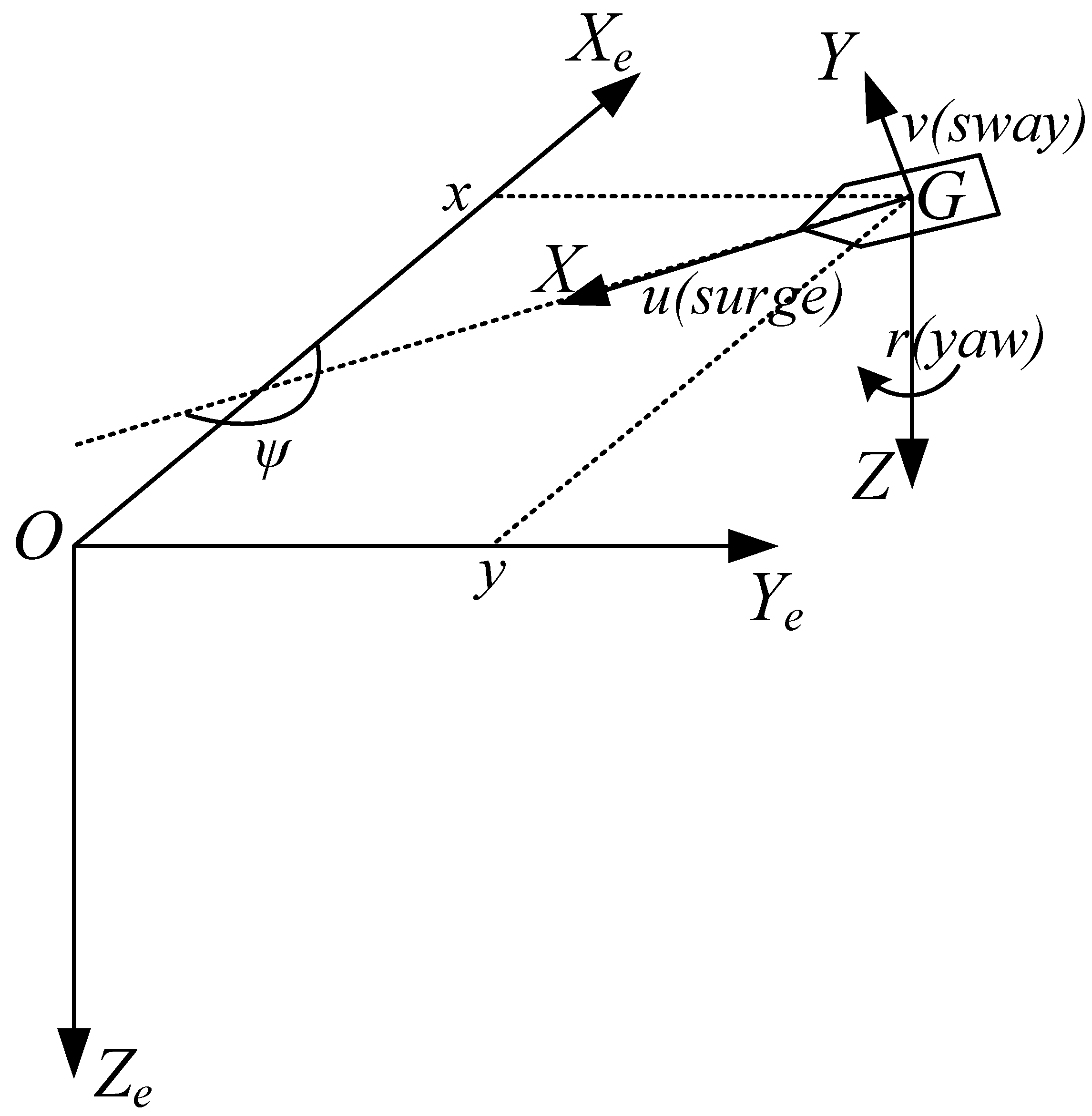
The earth-fixed coordinate system OX_eY_eZ_e and the body-fixed coordinate system GXYZ must be introduced to establish the mathematical model of ship motions. These two systems are shown in Figure 1. The origin O of the Earth-fixed coordinate system is any point on the earth’s surface. The axes of OX_e, OY_e, and OZ_e point to the north, east, and spherical center of the earth, respectively. The body-fixed coordinate system adheres to the ship with its origin G set at the center of gravity. The GX axis points to the ship’s bow direction, the GY axis is perpendicular to the GX axis and points to the ship’s starboard, and the GZ axis points to the spherical center of the earth.

Figure 1. Earth-Fixed Coordinate System and Body-Fixed Coordinate System.

When the DP ship performs the trajectory tracking task, ship motion generally consists of the surge, sway, and yaw (seen in Figure 1). Consequently, the ship’s motion can be deemed as 3-DOF (degree-of-freedom) motion. The 3-DOF kinematics model of the DP ship is defined as [1]:

$$\dot{\eta }=R(\psi )$$

(1)

where $\eta ={\left[\begin{array}{ccc}x& y& \psi \end{array}\right]}^T$ refers to the ship attitude vector in the earth-fixed coordinate system, in which (x,y) is ship position and ψ is the heading of the ship; $v={\left[\begin{array}{ccc}u& v& r\end{array}\right]}^T$ denotes the ship speed vector in the body-fixed coordinate system, in which u is surge speed, v is sway speed, and r is yaw rate; R(ψ) is the rotation matrix described by

$$R(\psi )=\left[\begin{array}{ccc}\cos \psi & -\sin \psi & 0\\ \sin \psi & \cos \psi & 0\\ 0& 0& 1\end{array}\right]$$

(2)

The dynamic model of the DP ship is defined below [1]:

$$M\dot{v}=-Dv+\tau +d$$

(3)

where $\tau ={\left[\begin{array}{ccc}{\tau }_x& {\tau }_y& {\tau }_N\end{array}\right]}^T$ is the control input vector expressed by force and torque generated by thrusters; $d={\left[\begin{array}{ccc}{d}_x& d_y& d_N\end{array}\right]}^T$ denotes the environmental disturbances; M is the inertia matrix presenting the sum of the ship’s mass and added mass; D indicates the damping coefficient matrix. These two matrices are written as

$$M=\left[\begin{array}{ccc}m-X_{\dot{u}}& 0& 0\\ 0& m-Y_{\dot{v}}& -Y_{\dot{r}}\\ 0& -N_{\dot{v}}& I_z-N_{\dot{r}}\end{array}\right]$$

(4)

$$D=\left[\begin{array}{ccc}-X_u& 0& 0\\ 0& -Y_v& -Y_r\\ 0& -N_v& -N_r\end{array}\right]$$

(5)

Remark 1: This paper focuses on low-speed trajectory tracking, so each hydrodynamic derivate in matrix D is linear. Additionally, the DP ship is fully actuated, for which τ_y may not be zero.

To facilitate the subsequent controller design, we can describe the mathematical model of the DP ship at low speed by combining Equations (1) and (3)

$$\dot{\zeta }=\left[\begin{array}{cc}{0}_{3\times 3}& R(\psi )\\ 0_{3\times 3}& -M^{-1}D\end{array}\right]\zeta +\left[\begin{array}{c}{0}_{3\times 3}\\ M^{-1}\end{array}\right]\tau +\left[\begin{array}{c}{0}_{3\times 3}\\ M^{-1}\end{array}\right]d=f(\zeta ,\tau ,d)$$

(6)

where the state variable is $\zeta ={\left[\begin{array}{llllll}x\hfill & y\hfill & \psi \hfill & u\hfill & v\hfill & r\hfill \end{array}\right]}^T$.

2.2. Problem Formulation

Consider a reference trajectory $p_d(t)={\left[\begin{array}{llllll}{x}_d(t)\hfill & y_d(t)\hfill & {\psi }_d(t)\hfill & u_d(t)\hfill & v_d(t)\hfill & r_d(t)\hfill \end{array}\right]}^T$, and the tracking error ζ_e is described as ${\zeta }_e=\zeta -p_d={\left[\begin{array}{llllll}{x}_e\hfill & y_e\hfill & {\psi }_e\hfill & u_e\hfill & v_e\hfill & r_e\hfill \end{array}\right]}^T$. The control objective in this paper is to design an anti-disturbance controller for the perturbed DP ship (Equation (6)) with control input constraints and speed state (u, v, and r) constraints such that the DP ship can accomplish the trajectory tracking task accurately. In other words, trajectory tracking error ζ_e should converge to a neighborhood of the origin.

Commonly, the control input constraints include two aspects: saturation of control inputs and saturation of the rate of change in control inputs. These two kinds of saturation are caused by the physical limits of ship thrusters. As this paper focuses on low-speed trajectory tracking, the speed state constraints have to be considered. These constraints can be set based on the suggestions of DP operators and general knowledge about DP ships.

To facilitate the controller design, some assumptions are considered as follows:

Assumption 1: p_d(t) and time derivatives of p_d(t) are smooth and bounded.

Assumption 2: Environmental disturbances have limited energies and generally vary slowly over time. As such, values of disturbances and time derivatives of disturbances are bounded..

3. ADLMPC of Low-Speed Trajectory Tracking Based on ESO

An MPC controller is a natural choice for the objective above due to its capability to handle constraints. Considering its recursive feasibility, closed-loop stability, and anti-disturbance ability, a novel ADLMPC scheme of low-speed trajectory tracking is developed by integrating LMPC with ESO. Figure 2 shows the architecture of the novel trajectory tracking control scheme.

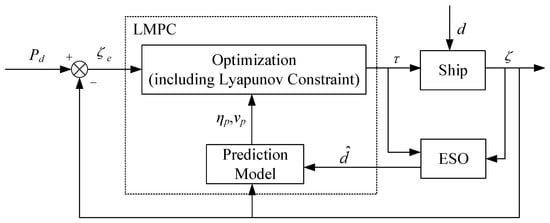
Figure 2. ADLMPC Scheme of Trajectory Tracking.

In the ADLMPC scheme, ESO can estimate environmental disturbances d. The prediction model can provide predictive state ${\zeta }_p={\left[\begin{array}{ll}{\eta }_p^T\hfill & v_p^T\hfill \end{array}\right]}^T$ over the prediction horizon and be updated online through estimated environmental disturbances $\widehat{d}$, improving the prediction capability and control performance. The optimization module can determine the control input τ based on tracking error ζ_e and predictive state ζ_P. Moreover, the Lyapunov contraction constraint is added to the optimization module to guarantee closed-loop stability.

3.1. ESO Design

To facilitate the design of the ESO, Equation (3) can be rewritten as

$$\dot{v}=-M^{-1}Dv+M^{-1}\tau +M^{-1}d$$

(7)

The ESO can be developed for Equation (7) as

$$\{\begin{array}{l}\dot{\widehat{v}}=-M^{-1}Dv+M^{-1}\widehat{d}+M^{-1}\tau -{\beta }_1(\widehat{v}-v)\hfill \\ \dot{\widehat{d}}=-{\beta }_2(\widehat{v}-v)\hfill \end{array}$$

(8)

where $\widehat{v}$ and $\widehat{d}$ are estimations of v and d, respectively; ${\beta }_1\in R^{3\times 3}$ and ${\beta }_2\in R^{3\times 3}$ are observer gain matrices that can be designed. Let the speed estimation error and the disturbance estimation error be $\tilde{v}=v-\widehat{v}$ and $\tilde{d}=d-\widehat{d}$, respectively. Considering Assumption 2, the estimation errors above can converge to a neighborhood of the origin by determining appropriate β₁ and β₂. Details of the proof can be seen in [33].

3.2. ADLMPC Controller Design

Based on the ESO and the control objective in Section 2, the optimization problem at time t₀ can be defined by

$$\underset{{\tau }_{mpc}}{\min }J={\displaystyle {\int }_{t_0}^{t_0+N}({\Vert {\zeta }_e(t)\Vert }_Q^2+{\Vert {\tau }_{mpc}(t)\Vert }_R^2)dt}$$

(9a)

$$\mathrm{s}.\mathrm{t}. \dot{\zeta }(t)=f(\zeta (t),{\tau }_{mpc}(t),\widehat{d}(t))$$

(9b)

$${\tau }_{\min }\le {\tau }_{mpc}\le {\tau }_{\max }$$

(9c)

$${\dot{\tau }}_{\min }\le {\dot{\tau }}_{mpc}\le {\dot{\tau }}_{\max }$$

(9d)

$$v_{\min }\le v\le v_{\max }$$

(9e)

$$\dot{V}(\zeta (t_0),{\tau }_{mpc}(t_0),\widehat{d}(t_0))\le \dot{V}(\zeta (t_0),{\tau }_{vir}(t_0),\widehat{d}(t_0))$$

(9f)

where N denotes the prediction horizon and Q and R represent weighting matrices which are diagonal and positive-definite. In detail, Q can be adjusted to specify the emphasis placed on the trajectory tracking error of particular states, while R can be tuned to describe the energy cost of the control inputs. For example, if a high precision of trajectory tracking is needed, the values of elements in Q can be set large. Additionally, if energy consumption is limited in some cases, the values of elements in R can be set large. τ_mpc is the control input produced by the ADLMPC controller; τ_max and τ_min are the maximum and minimum τ_mpc; ${\dot{\tau }}_{\max }$ and ${\dot{\tau }}_{\min }$ are the maximum and minimum change rates of τ_mpc. Equation (9e) means the constraints of ship speed states u, v, and r, due to the DP ship, are tracking trajectory at low speed. Equation (9f) is the Lyapunov contraction constraint which exploits a virtual Lyapunov-based trajectory tracking control law τ_vir. It should be noted that τ_vir does not actually control the DP ship but only guarantees closed-loop stability. V(·) is the corresponding Lyapunov function candidate for Equation (6).

Remark 2: Equation (9a–9f) has to be discretized first to solve the optimization problem numerically.

Then, we need to design τ_vir and V properly. Many techniques, such as sliding mode control, backstepping, and dynamic surface control, can be utilized to develop τ_vir. Considering the complexity of the controlled system and input constraints, we incorporate the auxiliary dynamic system into the backstepping technique to develop τ_vir.

Define the following variables:

$$e=\eta -{\eta }_d$$

(10)

$$\delta =v-v_d$$

(11)

where $e\in R^3$ and $\delta \in R^3$ are position error and speed error, respectively; ${\eta }_d={\left[\begin{array}{ccc}{x}_d& y_d& {\psi }_d\end{array}\right]}^T$ denotes reference position; and $v_d\in R^3$ is intermediate control.

By differentiating both sides of Equation (10), we can obtain

$$\dot{e}=R(\psi )(v_d+\delta )-{\dot{\eta }}_d$$

(12)

In order to stabilize Equation (10), v_d can be designed as follows:

$$v_d=R^{-1}(\psi )({\dot{\eta }}_d-K_{1}e)$$

(13)

where $K_1\in R^{3\times 3}$ is a specified control gain matrix that is positive-definite and diagonal.

From Equations (7) and (10), the time derivative of δ is

$$\dot{\delta }=M^{-1}(-Dv+d+{\tau }_c+\Delta \tau )-{\dot{v}}_d$$

(14)

where τ_c denotes the command control input without consideration of input constraints; $\Delta \tau ={\tau }_{vir}-{\tau }_c$ is the error between command control law and virtual control law which satisfies input constraints. To weaken the impact of Δτ on control performance, we introduce the following auxiliary dynamic system [34]:

$$M\dot{\xi }=-K_2\xi +\Delta \tau$$

(15)

where $K_2\in R^{3\times 3}$ is a specified control gain matrix which is positive-definite and diagonal; $\xi \in R^3$ is the state of the auxiliary dynamic system.

Based on ξ, the new speed error $\overline{\delta }$ considering input constraints is defined as

$$\overline{\delta }=\delta -\xi$$

(16)

Considering Equations (14) and (15), the time derivative of $\overline{\delta }$ becomes

$$\dot{\overline{\delta }}=M^{-1}(-Dv+d+{\tau }_c+K_2\xi )-{\dot{v}}_d$$

(17)

In order to stabilize Equation (17), τ_c can be designed below

$${\tau }_c=Dv-\widehat{d}+M{\dot{v}}_d-K_2\xi -K_3\overline{\delta }-R^T(\psi )e$$

(18)

where $K_3\in R^{3\times 3}$ is a specified control gain matrix that is positive-definite and diagonal.

According to Equations (9c), (9d) and (18), τ_vir can be presented as

$${\tau }_{vir}(t)=sa{t}_M({\tau }_{vir}(t-h)+h\times sa{t}_R(({\tau }_c(t)-{\tau }_{vir}(t-h))/h))$$

(19)

where h denotes the sampling period; $sa{t}_M(\tau (t))=\{\begin{array}{l}{\tau }_{\max },\tau (t)>{\tau }_{\max }\hfill \\ \tau (t),{\tau }_{\min }<\tau (t)<{\tau }_{\max }\hfill \\ {\tau }_{\min },\tau (t)<{\tau }_{\min }\hfill \end{array}$ is the saturation function of the control input, and $sa{t}_R(\tau (t))=\{\begin{array}{l}{\dot{\tau }}_{\max },\dot{\tau }(t)>{\dot{\tau }}_{\max }\hfill \\ \dot{\tau }(t),{\dot{\tau }}_{\min }<\dot{\tau }(t)<{\dot{\tau }}_{\max }\hfill \\ {\dot{\tau }}_{\min },\dot{\tau }(t)<{\dot{\tau }}_{\min }\hfill \end{array}$ is the saturation function of the change rate of the control input.

The Lyapunov function candidate V for Equation (6) is designed below:

$$V=\frac{1}{2}{e}^{T}e+\frac{1}{2}{\overline{\delta }}^{T}M\overline{\delta }+\frac{1}{2}{\xi }^{T}M\xi$$

(20)

By differentiating both sides of Equation (20), the following equation can be obtained:

$$\dot{V}=e^T\dot{e}+{\overline{\delta }}^{T}M\dot{\overline{\delta }}+{\xi }^{T}M\dot{\xi }$$

(21)

Based on Equations (12), (13), (15), (17), (18) and (21), the right-hand side of Equation (9f) can be modified to

$$\begin{array}{cc}\dot{V}(\zeta (t_0),{\tau }_{vir}(t_0),\widehat{d}(t_0))& =-e^T{K}_{1}e-{(\delta -{\xi }_{vir})}^T{K}_3(\delta -{\xi }_{vir})\hfill \\ & -{\xi }_{vir}^T{K}_2{\xi }_{vir}+e^{T}R(\psi ){\xi }_{vir}+{\xi }_{\mathrm{vir}}^T({\tau }_{vir}-{\tau }_c)\hfill \end{array}$$

(22)

where ξ_vir is the state of the auxiliary dynamic system affected by τ_vir.

According to Equations (7), (12), (15), (17) and (21), the left-hand side of Equation (9f) can be described as

$$\begin{array}{cc}\dot{V}(\zeta (t_0),{\tau }_{mpc}(t_0),\widehat{d}(t_0))=& e{(t_0)}^T(R(\psi (t_0))v(t_0)-{\dot{\eta }}_d(t_0))\hfill \\ & +{(\delta (t_0)-{\xi }_{mpc}(t_0))}^T(-Dv(t_0)+\widehat{d}(t_0)+{\tau }_c(t_0)-M{\dot{v}}_d(t_0)\hfill \\ & +K_2{\xi }_{mpc}(t_0))+{\xi }_{mpc}{(t_0)}^{T}M{\dot{\xi }}_{mpc}(t_0)\hfill \end{array}$$

(23)

where ξ_mpc is the state of the auxiliary dynamic system affected by τ_mpc.

Therefore, the expression of Equation (9e) is

$$\begin{array}{l}e{(t_0)}^T(R(\psi (t_0))v(t_0)-{\dot{\eta }}_d(t_0))\\ +{(\delta (t_0)-{\xi }_{mpc}(t_0))}^T(-Dv(t_0)+\widehat{d}(t_0)+{\tau }_c(t_0)-M{\dot{v}}_d(t_0)\\ +K_2{\xi }_{mpc}(t_0))+{\xi }_{mpc}{(t_0)}^{T}M{\dot{\xi }}_{mpc}(t_0)\\ \le -e{(t_0)}^T{K}_{1}e(t_0)-{(\delta (t_0)-{\xi }_{vir}(t_0))}^T{K}_3(\delta (t_0)-{\xi }_{vir}(t_0))\\ -{\xi }_{vir}^T(t_0)K_2{\xi }_{\mathrm{vir}}(t_0)+e{(t_0)}^{T}R(\psi (t_0)){\xi }_{vir}(t_0)\\ +{\xi }_{vir}^T(t_0)({\tau }_{vir}(t_0)-{\tau }_c(t_0))\end{array}$$

(24)

3.3. Stability Analysis

In the last section, the Lyapunov contraction constraint (Equation (24)) is established, but the choice of control gain matrices K₁, K₂, and K₃ is not discussed. To satisfy the recursive feasibility of ADLMPC and closed-loop stability, we analyze the selection guidelines of K₁, K₂, and K₃ in this section.

Theorem 1.

Provided that control gain matrices K₁, K₂, and K₃ ensure ${\lambda }_{\min }\left(K_1\right)>\frac{1}{2}$, ${\lambda }_{\min }\left(K_2\right)>1$, and ${\lambda }_{\min }\left(K_3\right)>0$, the command control input τ_c (Equation (18)) designed for the mathematical model of the DP ship (Equation (6)) can guarantee the uniform ultimate boundedness of all signals in the trajectory tracking control system under virtual control law τ_vir.

Proof .

According to Young’s inequality and Equation (22), the following inequality can be obtained:

$$\begin{array}{c}\dot{V}\le -e^T{K}_{1}e-{\overline{\delta }}^T{K}_3\overline{\delta }-{\xi }^T{K}_2\xi +\frac{1}{2}{e}^{T}e+\frac{1}{2}{\xi }^T\xi +\frac{1}{2}{\xi }^T\xi +\frac{1}{2}\Delta {\tau }^T\Delta \tau \hfill \\ =-e^T(K_1-\frac{1}{2}{I}_{3\times 3})e-{\overline{\delta }}^T{K}_3\overline{\delta }-{\xi }^T(K_2-I_{3\times 3})\xi +\frac{1}{2}{\Vert \Delta \tau \Vert }^2\hfill \\ \le -({\lambda }_{\min }(K_1)-\frac{1}{2})e^{T}e-{\lambda }_{\min }(K_3){\overline{\delta }}^T\overline{\delta }-({\lambda }_{\min }(K_2)-1){\xi }^T\xi +\frac{1}{2}{\Vert \Delta \tau \Vert }^2\hfill \\ \le -2\mu V+C\hfill \end{array}$$

(25)

where $\mu =\min \left\{{\lambda }_{\min }(K_1)-\frac{1}{2},{\lambda }_{\min }(K_3)/{\lambda }_{\max }(M),({\lambda }_{\min }(K_2)-1)/{\lambda }_{\max }(M)\right\}$ and $C=\frac{1}{2}{\Vert \Delta \tau \Vert }^2$. □

To solve Equation (25), we can obtain

$$0\le V(t)\le \frac{C}{2\mu }+(V(t_0)-\frac{C}{2\mu })e^{-2\mu t}$$

(26)

Equation (26) indicates that if $\mu >0$ then ${\lambda }_{\min }(K_1)>\frac{1}{2}$, ${\lambda }_{\min }(K_2)>1$, and ${\lambda }_{\min }(K_3)>0$, $\underset{t\to \infty }{\lim }V{(t)}_{\max }=\frac{C}{2\mu }$. Therefore, V(t) is uniformly ultimately bounded. In accordance with Equation (20), we can judge the uniform ultimate boundedness of e, $\overline{\delta }$, and ξ. Further consideration of Assumption 1 together with Equations (10), (11), (13) and (16) concludes that the uniform ultimate boundedness of η, v, and v_d are all satisfied, which completes the proof.

Then, we analyze the recursive feasibility of ADLMPC and closed-loop stability of the system controlled by τ_mpc. Input constraints are considered in the design of virtual control law τ_vir(t) in ADLMPC. Therefore τ_vir(t) is always the feasible solution of Equation (9), which naturally satisfies the recursive feasibility. In terms of closed-loop stability, the following inequality can be obtained based on Equations (9f) and (25):

$$\dot{V}(\zeta (t_0),{\tau }_{mpc}(t_0),\widehat{d}(t_0))\le \dot{V}(\zeta (t_0),{\tau }_{vir}(t_0),\widehat{d}(t_0))\le -2\mu V+C$$

(27)

The solution of Equation (27) is similar to Equation (26), which means the uniform ultimate boundedness of all signals in the trajectory tracking control system are satisfied under the MPC control law τ_mpc.

4. Simulation Results

In this section, comparative simulations of the trajectory tracking of the model DP ship using Matlab are conducted to verify the efficacy and superiorities of the proposed ADLMPC scheme. The parameters for the model DP ship are taken from a supply vessel named Northern Clipper [35].

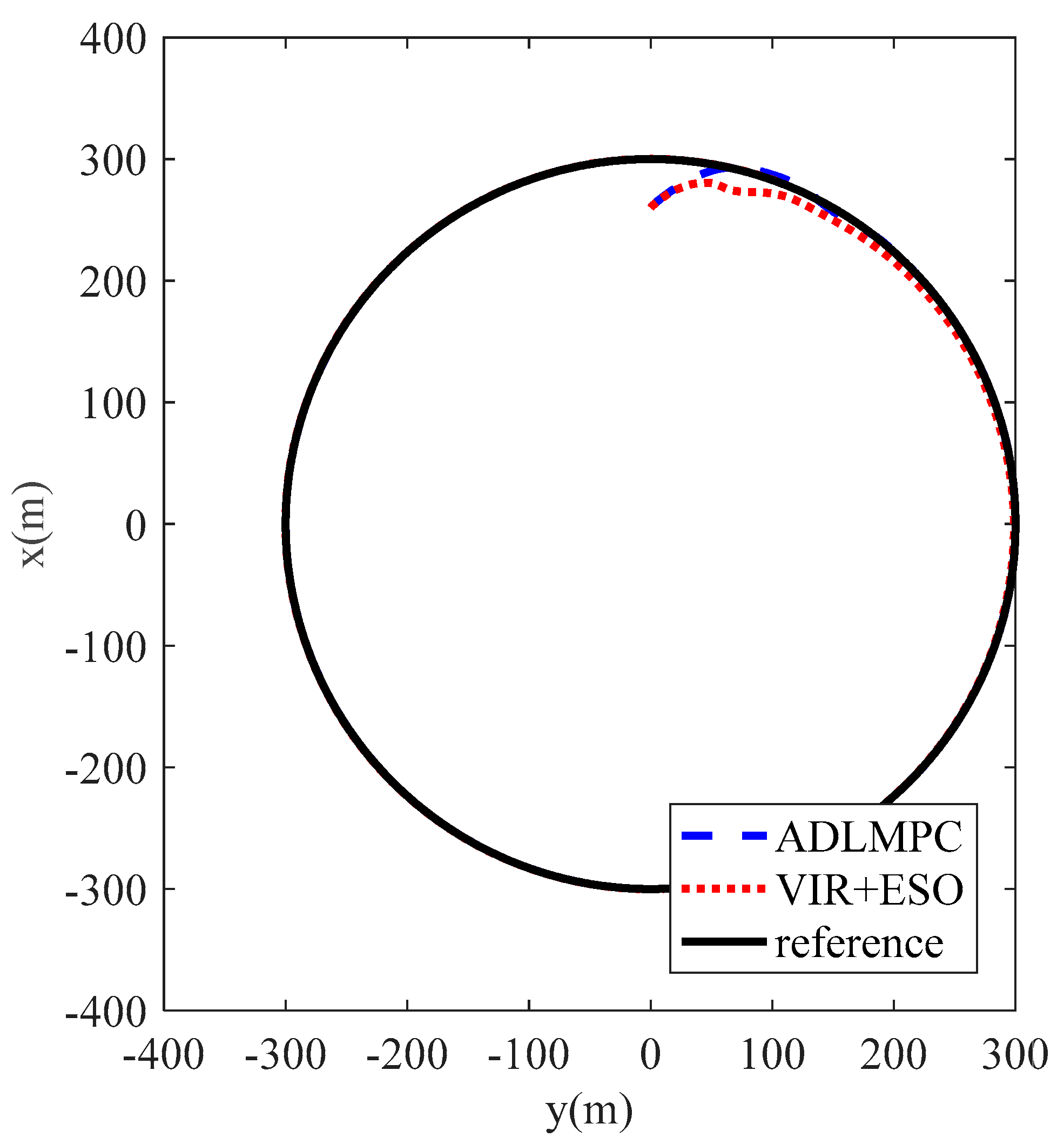
The reference trajectory adopted in simulation case 1 is a circular trajectory defined by

$$p_d(t)=\{\begin{array}{l}{x}_d=300\cos (0.0067t)\hfill \\ y_d=300\sin (0.0067t)\hfill \\ {\psi }_d=a\tan 2(3\cos (0.0067t),-3\sin (0.0067t))\hfill \\ u_d=2\hfill \\ v_d=0\hfill \\ r_d=0.0067\hfill \end{array}$$

(28)

The disturbance on the model ship in simulation case 1 is assumed to be $d(t)={\left[\begin{array}{ccc}6\times {10}^5\sin (0.05t)(N)& 1.8\times {10}^5\sin (0.05t)(N)& 4.4\times {10}^6\sin (0.05t)(N\cdot m)\end{array}\right]}^T$. The initial state of the model ship is $\zeta (0)={\left[\begin{array}{llllll}260(m)\hfill & 0(m)\hfill & 50\cdot \pi /180(rad)\hfill & 0(m/s)\hfill & 0(m/s)\hfill & 0(rad/s)\hfill \end{array}\right]}^T$. The upper bound and lower bound of speed states u, v, and r are set as ±3 m/s, ±2 m/s, and ±1°/s, respectively. The maximum and minimum force and torque generated by thrusters are ${\left[\begin{array}{ccc}-1\times {10}^{6}N& -3\times {10}^{5}N& -7.62\times {10}^{6}N\cdot m\end{array}\right]}^T$ and ${\left[\begin{array}{ccc}1\times {10}^{6}N& 3\times {10}^{5}N& 7.62\times {10}^{6}N\cdot m\end{array}\right]}^T$, respectively. The minimum and maximum change rates of force and torque are ${\left[\begin{array}{ccc}-2\times {10}^{5}N\cdot s^{-1}& -6\times {10}^{4}N\cdot s^{-1}& -1.524\times {10}^{6}N\cdot m\cdot s^{-1}\end{array}\right]}^T$ and ${\left[\begin{array}{ccc}2\times {10}^{5}N\cdot s^{-1}& 6\times {10}^{4}N\cdot s^{-1}& 1.524\times {10}^{6}N\cdot m\cdot s^{-1}\end{array}\right]}^T$.

For the ADLMPC controller in simulation case 1, the prediction horizon N and sampling period h are set to be 25 s and 0.5 s, respectively; weighting matrices are designed as $Q_1=diag\left\{3\times {10}^6,3\times {10}^6,5\times {10}^8,3\times {10}^6,3\times {10}^6,5\times {10}^{10}\right\}$ and $R_1=diag\left\{1\times {10}^{-10},1\times {10}^{-9},1\times {10}^{-11}\right\}$; control gain matrices are developed as $K_1=diag\left\{0.7,0.7,0.7\right\}$, $K_2=diag\left\{1\times {10}^5,1\times {10}^5,1\times {10}^8\right\}$ and $K_3=diag\left\{1\times {10}^7,1\times {10}^7,1\times {10}^{10}\right\}$; observer gain matrices in ESO are chosen as ${\beta }_1=diag\{0.4,1.6,1.2\}$ and ${\beta }_2=diag\{0.12,0.7,0.5\}$. The virtual controller developed through backstepping and an auxiliary dynamic system in ADLMPC is the comparative controller. The choices of control gain matrices are the same as those in the ADLMPC controller. Moreover, the ESO should be incorporated into the virtual controller to estimate and compensate for disturbances. The main reason for choosing the virtual controller as the comparative controller is that the control law generated by the virtual controller not only can make the ship track the reference trajectory, but also satisfies the control inputs constraints.

To solve the optimization control problem Equation (9) numerically, the software package called CasADi is selected. This package is developed to assist rapid and efficient implementation of different methods for numerical optimal control [36]. Due to Equation (9) being a quadratic programming problem, this package solves the problem using the sequential quadratic programming (SQP) method, using the IPOPT solver.

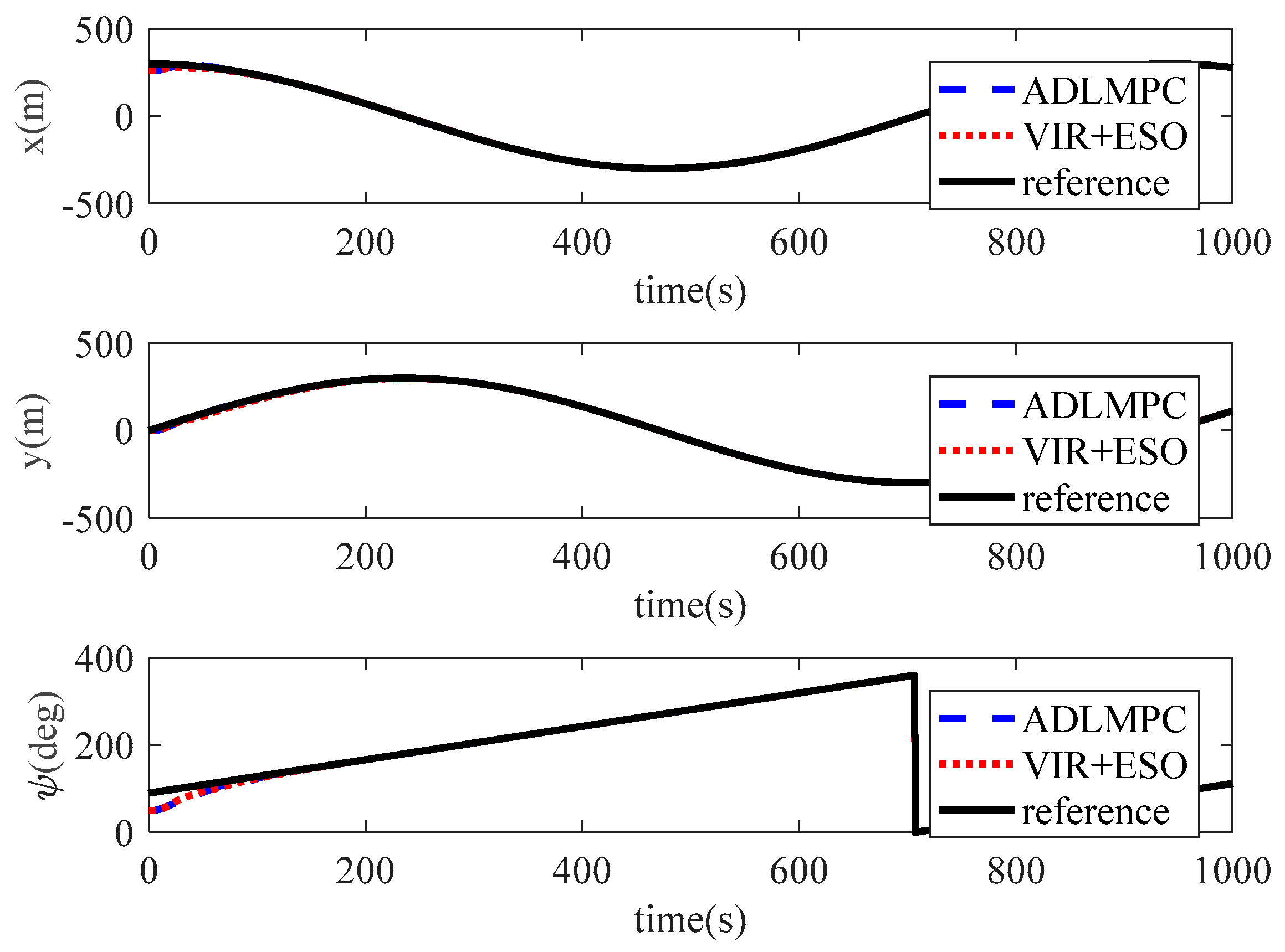
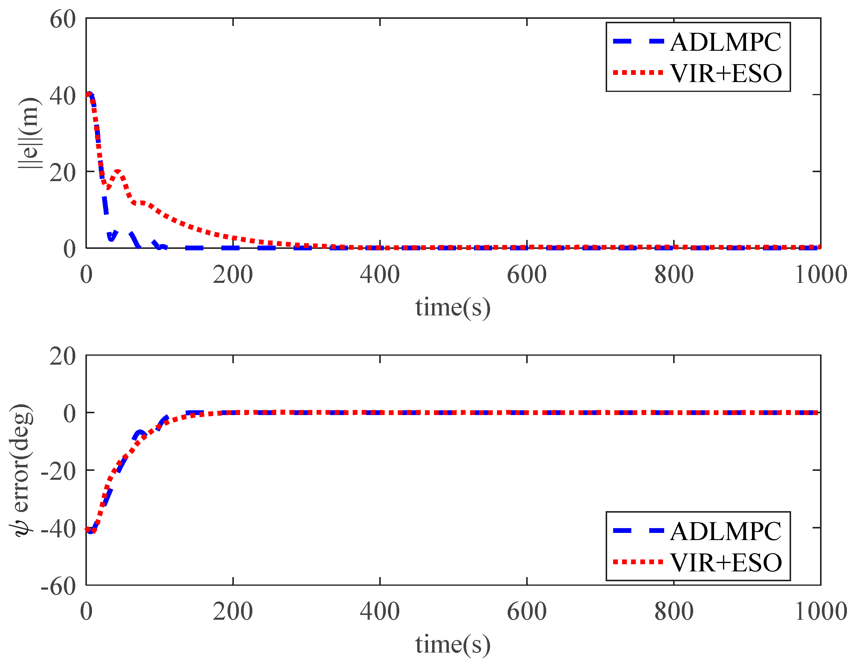
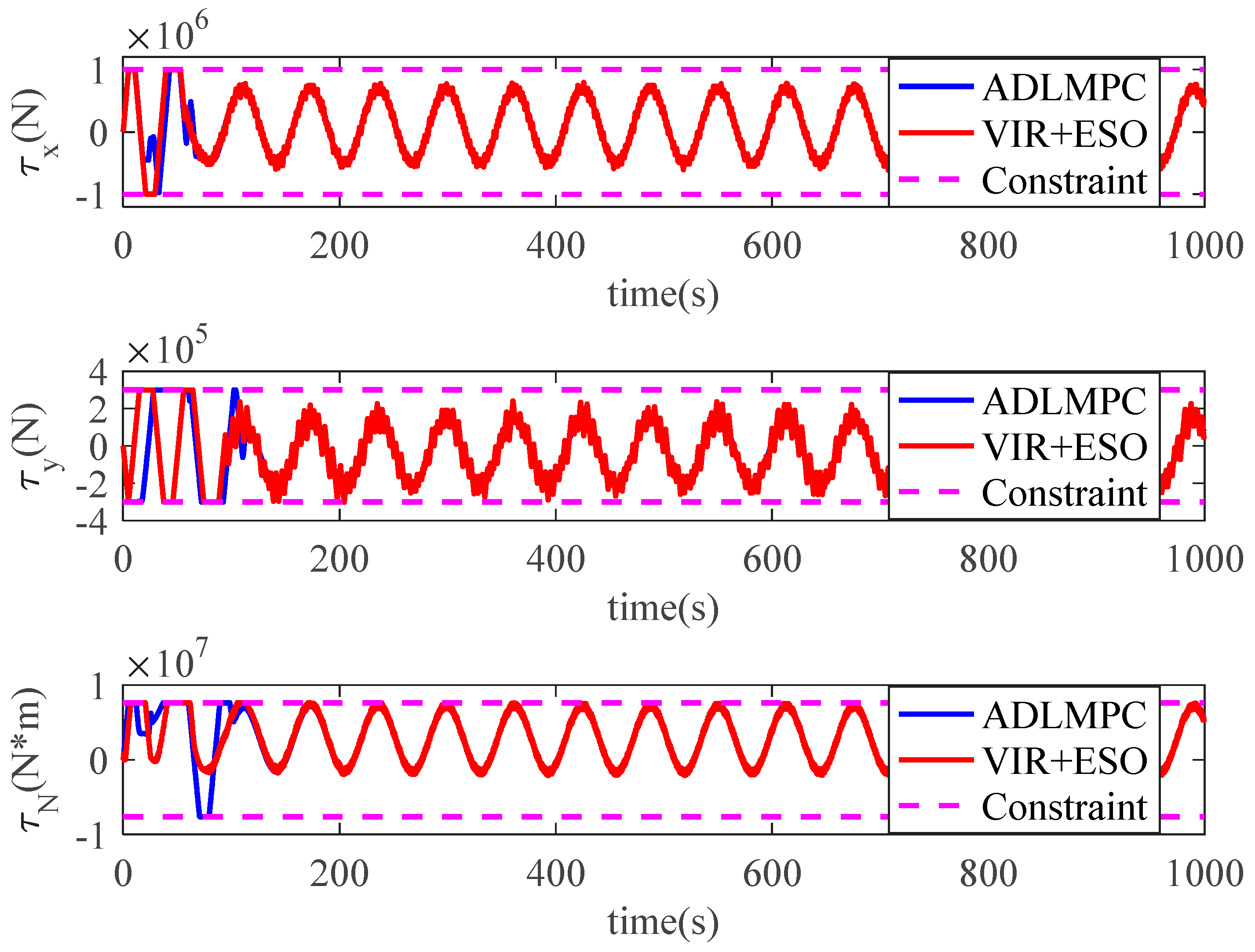
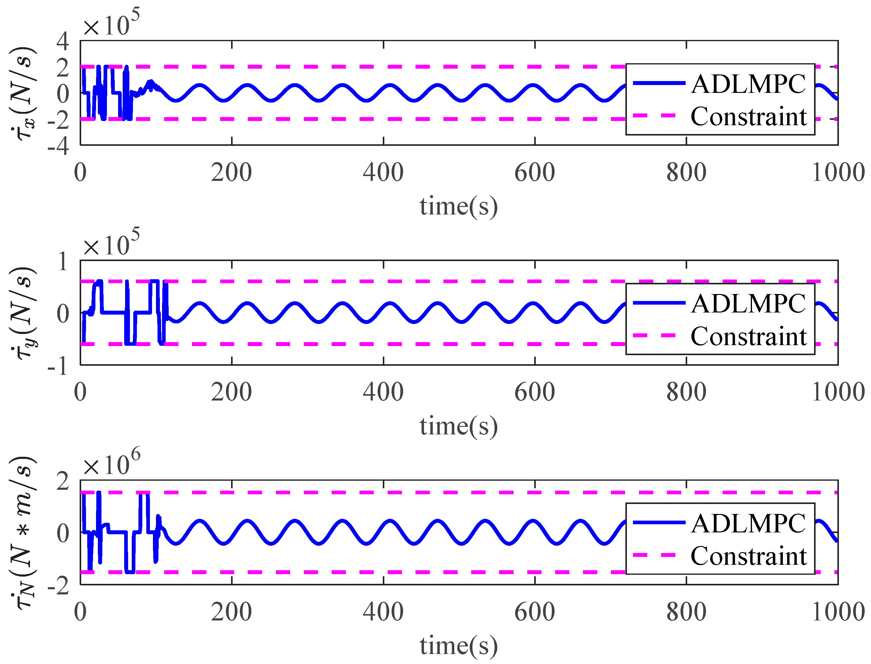
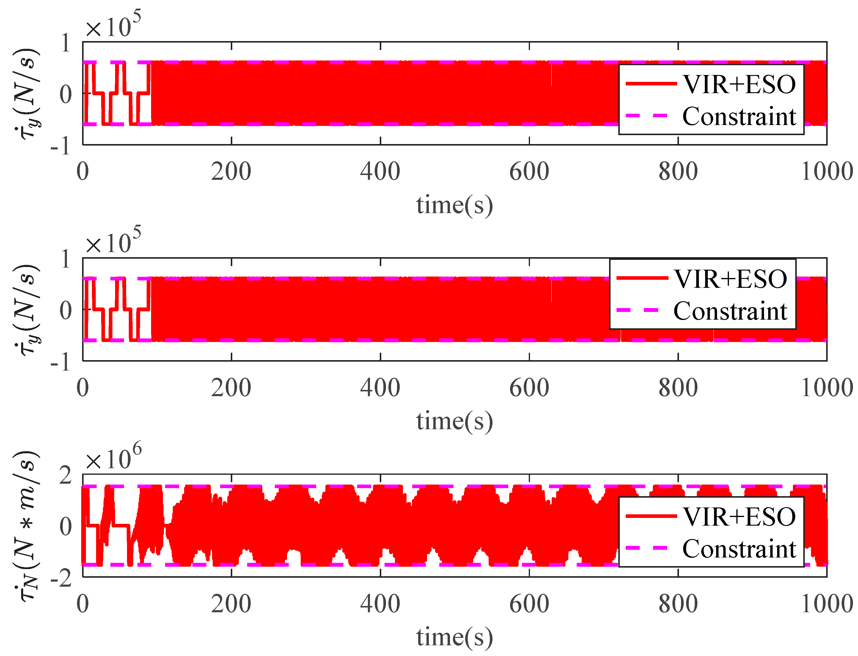
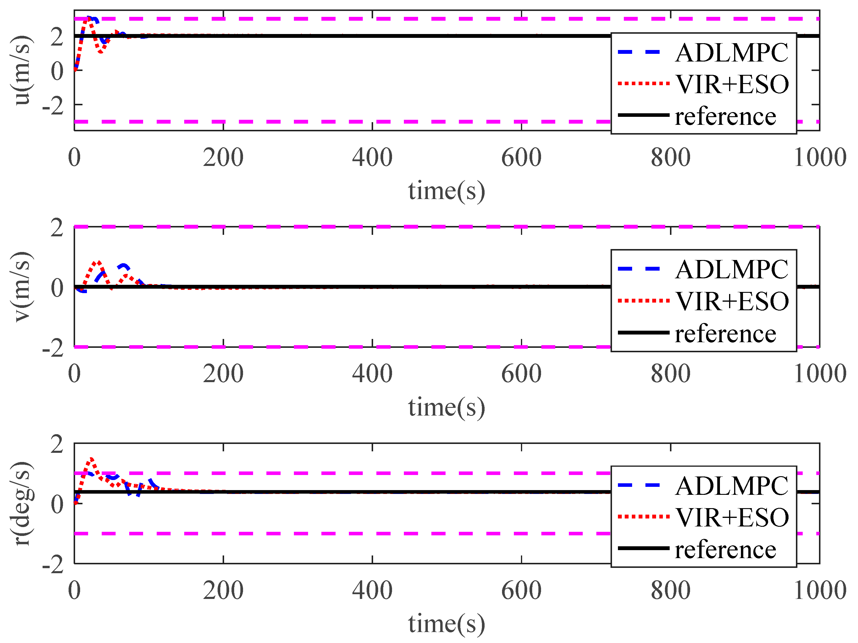
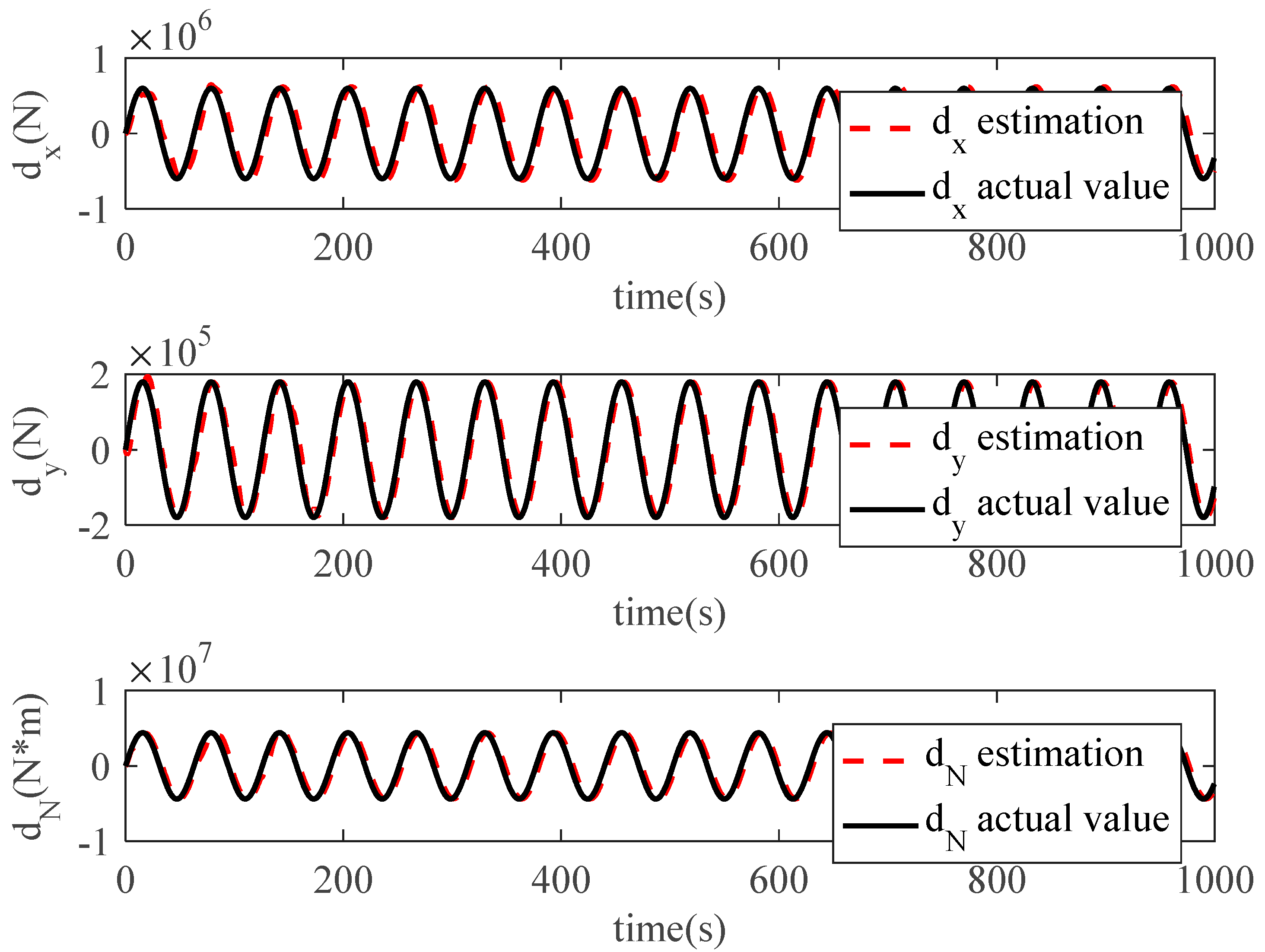
Simulation results of case 1 are presented in Figure 3, Figure 4, Figure 5, Figure 6, Figure 7, Figure 8, Figure 9 and Figure 10. Specifically, the ship trajectories controlled by the ADLMPC controller and comparative virtual controller with ESO (VIR+ESO) are illustrated in Figure 3 and Figure 4. As we can see, both controllers show high qualities of control performance, which can accurately control the model ship perturbed by environmental disturbances to track reference trajectory. However, Figure 3 illustrates that the model ship can track the reference trajectory more rapidly with the proposed ADLMPC controller. Meanwhile, Figure 4 demonstrates more detailed information. The position tracking error $e={\left[\begin{array}{cc}x-x_d& y-y_d\end{array}\right]}^T$ and the heading tracking error of both controllers are presented in Figure 5, which indicates that tracking errors resulting from both controllers converge to a small neighborhood of the origin. The efficacy and closed-loop stability of both controllers are verified. In detail, by the effect of ADLMPC and the virtual controller, the position tracking error achieves convergence in about 100 s and 300 s, and the corresponding steady-state error is near 0 and about 0.5 m. Moreover, the mean square errors (MSE) for both controllers are listed in Table 1. It can be seen from Table 1 that compared with the VIR+ESO, the MSEs of position states (x and y) with the proposed ADLMPC controller appear to have different degrees of decline. The improvements in the MSEs of position states with the ADLMPC controller are 20.2% and 73.5%, respectively. This information shows that no matter the accuracy of tracking or the convergence time, the ADLMPC controller’s tracking performance is better than the virtual controller, which mainly results from the optimization module in ADLMPC. This module can provide optimal or sub-optimal control law by solving the optimization problem online, which means that thrusters can be utilized more efficiently. Figure 6 and Figure 7 describe the control inputs of both controllers, from which we can observe that control inputs do not violate the input constraints. Additionally, the torque generated by the ADLMPC controller in the first 100 s is more significant than that generated by the virtual controller. This means that the ADLMPC controller fully utilizes the thrusters to track the reference trajectory rapidly. The rates of change in control inputs produced by both controllers also satisfy the control input constraint in Figure 8. However, the rates of change in control inputs generated by the virtual controller are much more severe, aggravating the wear of thrusters and reducing their lifetime. It can also be understood that the virtual controller has to frequently change the thrust to achieve a similar tracking performance as the ADLMPC controller. Figure 9 illustrates the variation of speed states (u, v, and r) over time. Although both controllers can control the model ship to track reference speed, the state of r controlled by the virtual controller is out of the upper limit in 14–32 s. The main reason is that the speed state constraints are not considered when designing the virtual controller. This highlights the advantage of the ADLMPC controller in tackling system constraints explicitly. The estimation performance of the designed ESO is plotted in Figure 10. It reveals that the designed ESO can accurately estimate the actual disturbances. Regarding the computing burden of the ADLMPC controller, the average calculation period of the optimization control problem Equation (9) is around 70 ms, which means that the ADLMPC has positive real-time performance.

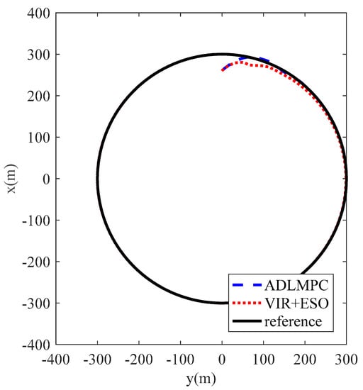
Figure 3. The trajectory of the DP ship controlled by ADLMPC and VIR+ESO.

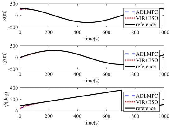
Figure 4. Position and heading variations of the DP ship controlled by ADLMPC and VIR+ESO.

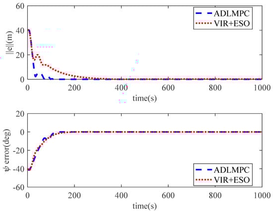
Figure 5. Tracking errors of position and heading controlled by ADLMPC and VIR+ESO.

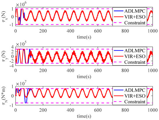
Figure 6. Control input generated by ADLMPC and VIR+ESO.

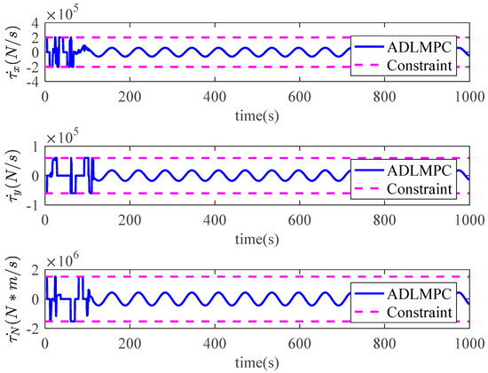
Figure 7. Rate of change in control input generated by ADLMPC.

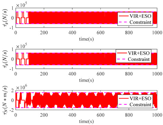
Figure 8. Rate of change in control input generated by VIR+ESO.

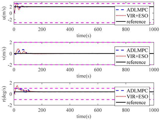
Figure 9. Speed states controlled by ADLMPC and VIR+ESO.

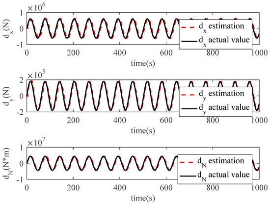
Figure 10. Estimations of environmental disturbances by ESO.

Table 1. Mean square errors of position states and heading state for case 1.

MSE	ADLMPC	VIR+ESO	Improvement
x (m2)	23.9584	30.0405	20.2%
y (m2)	4.1882	15.8001	73.5%
ψ (rad2)	0.0174	0.0175	0

To demonstrate the effects of the parameters for the ADLMPC controller on tracking performance, another simulation (simulation case 2) with a different set of parameters for the ADLMPC controller is performed. In this simulation case, the reference trajectory and environmental disturbances are the same as in case 1. However, the weighting matrices Q and R are changed to $Q_2=diag\left\{1\times {10}^2,1\times {10}^2,5\times {10}^5,1\times {10}^2,1\times {10}^2,5\times {10}^5\right\}$ and $R_2=diag\left\{1\times {10}^{-8},1\times {10}^{-7},1\times {10}^{-9}\right\}$. 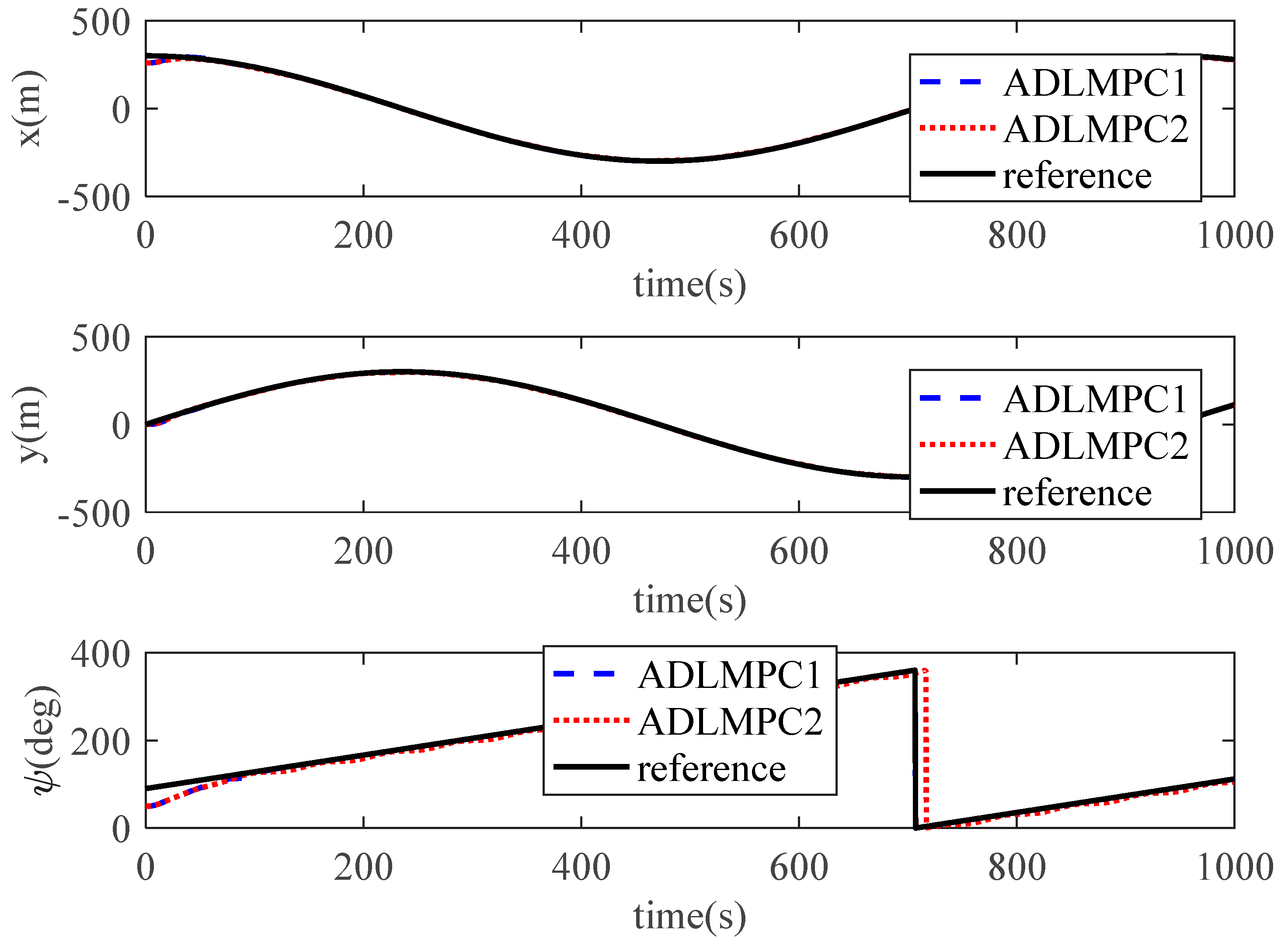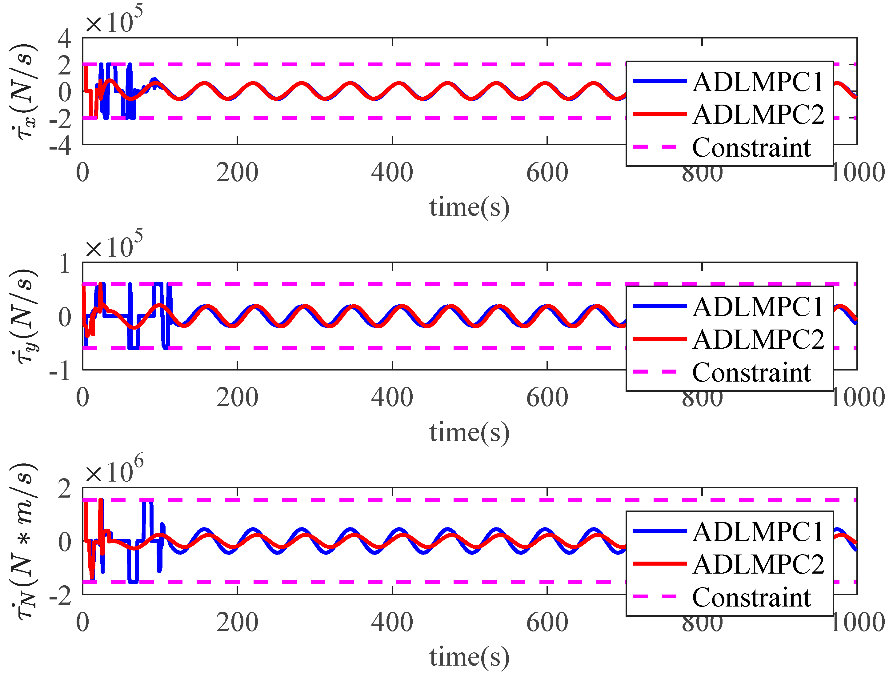The remaining parameters are maintained, including the prediction horizon, control gain matrices of the virtual controller, and observer gain matrices. The initial states of the model ship and environmental disturbances are also the same as those in case 1. Simulation results are shown in Figure 11, Figure 12, Figure 13, Figure 14, Figure 15 and Figure 16, and ‘ADLMPC1’ and ‘ADLMPC2’ in these figures mean the ADLMPC controller with weighting matrices Q₁, R₁, and with Q₂, R₁, respectively.

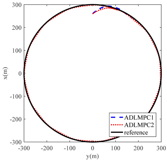
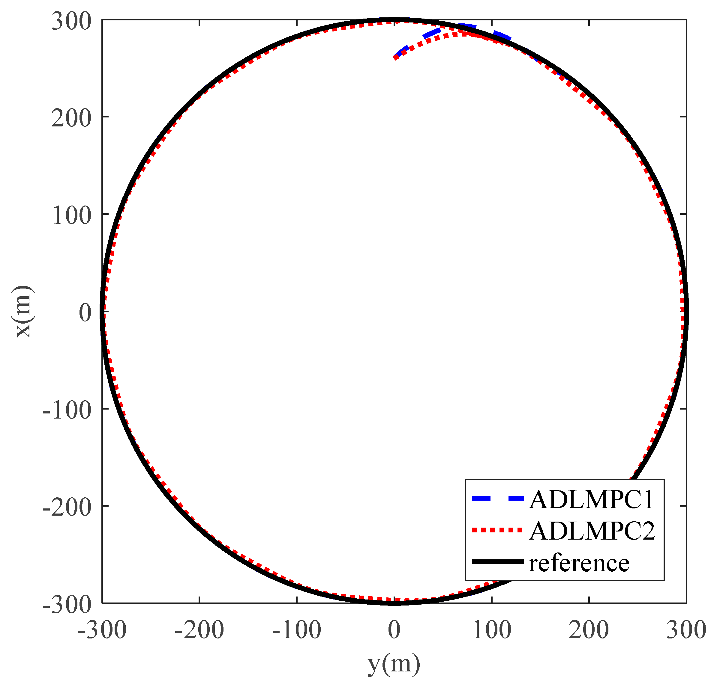
Figure 11. The trajectory of the DP ship controlled by ADLMPC1 and ADLMPC2.

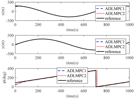
Figure 12. Position and heading variations of the DP ship controlled by ADLMPC1 and ADLMPC2.

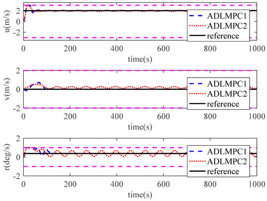
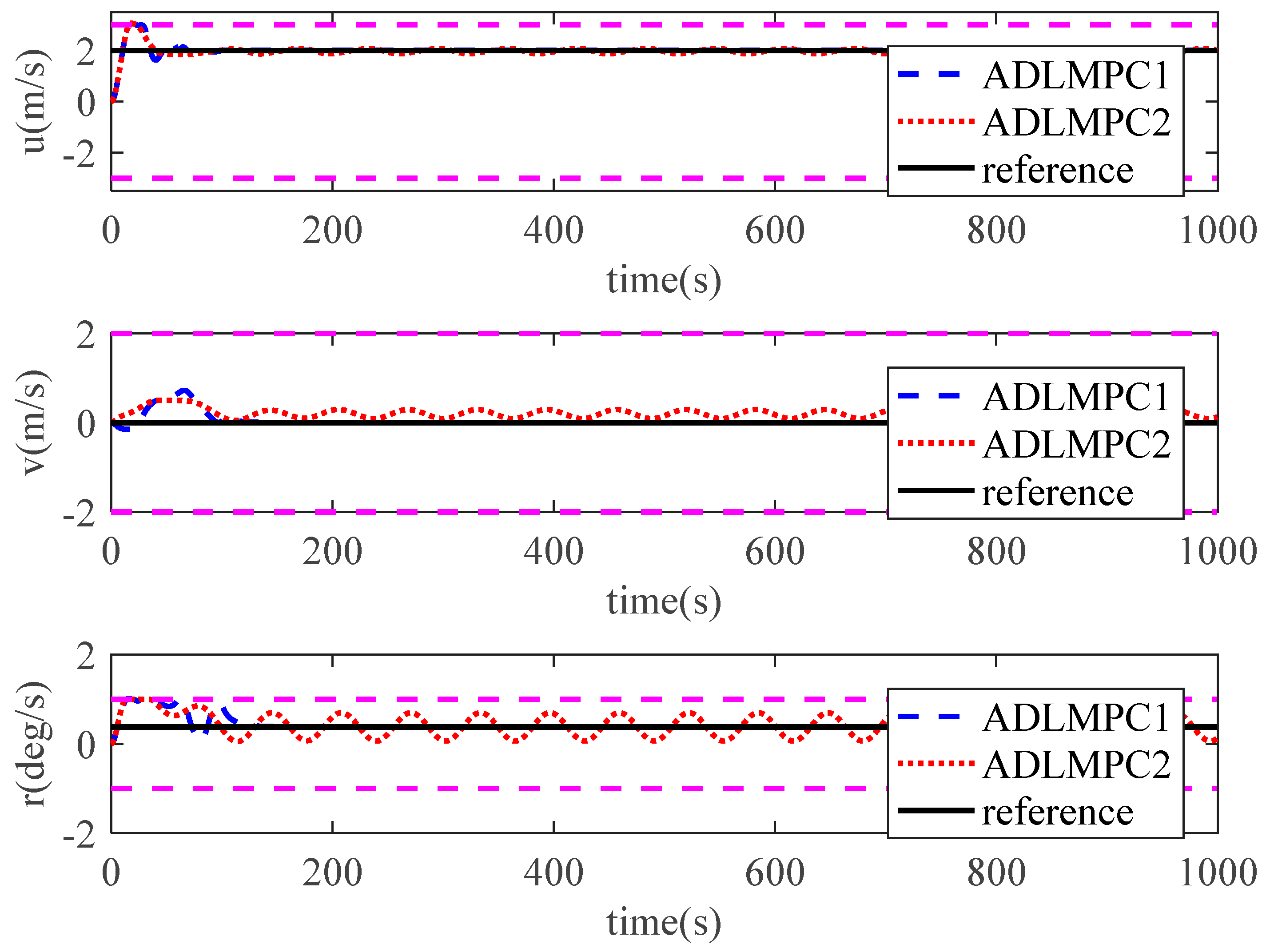
Figure 13. Speed states controlled by ADLMPC1 and ADLMPC2.

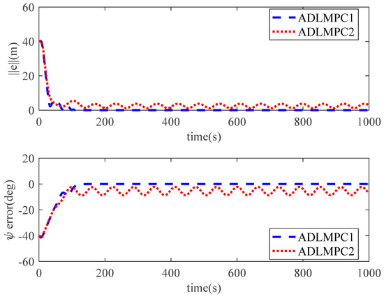
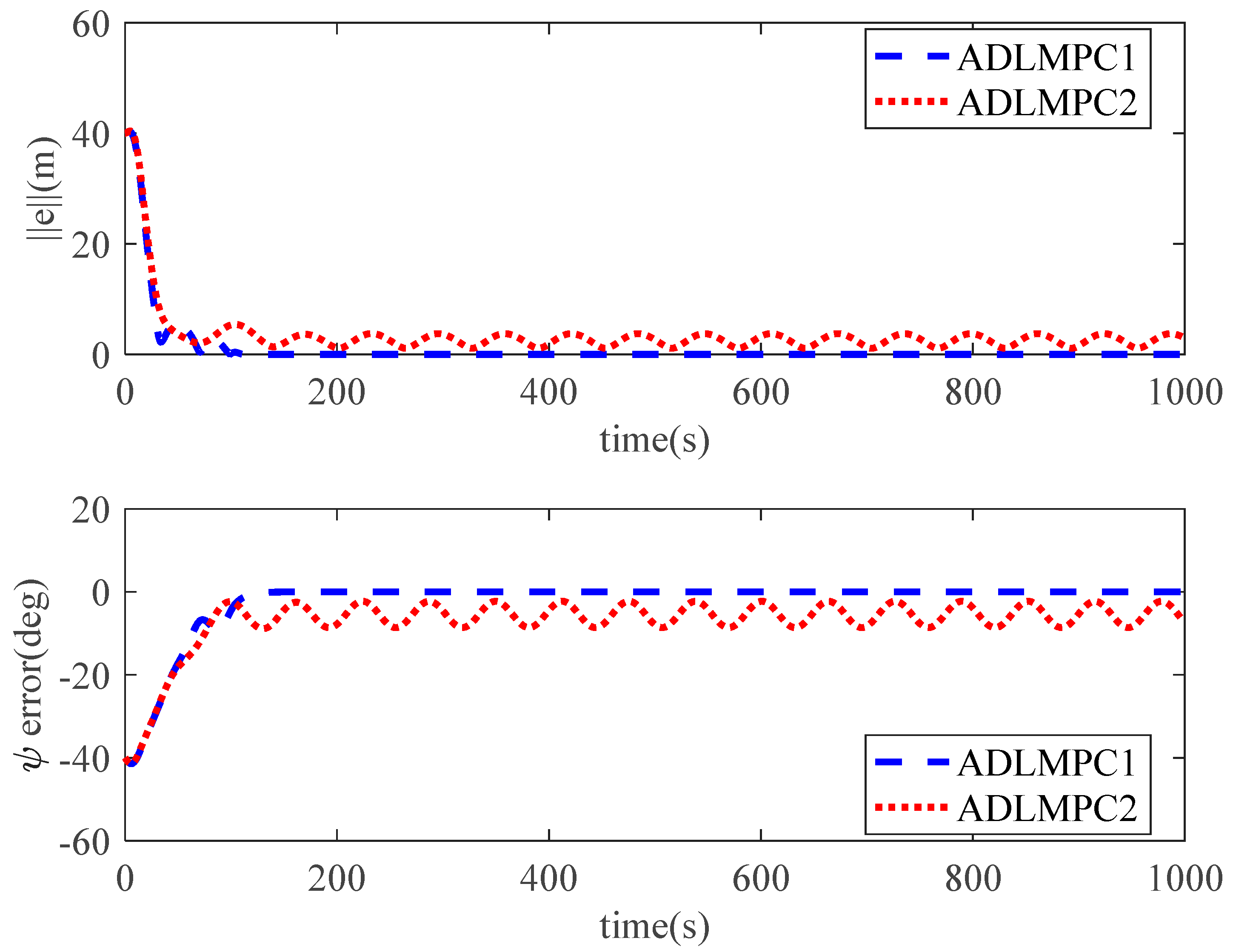
Figure 14. Tracking errors of position and heading controlled by ADLMPC1 and ADLMPC2.

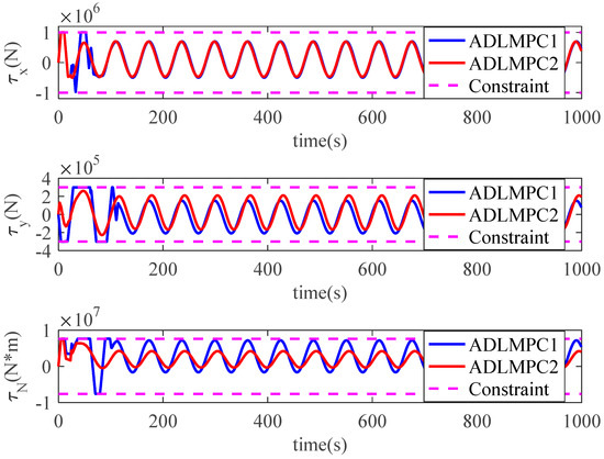
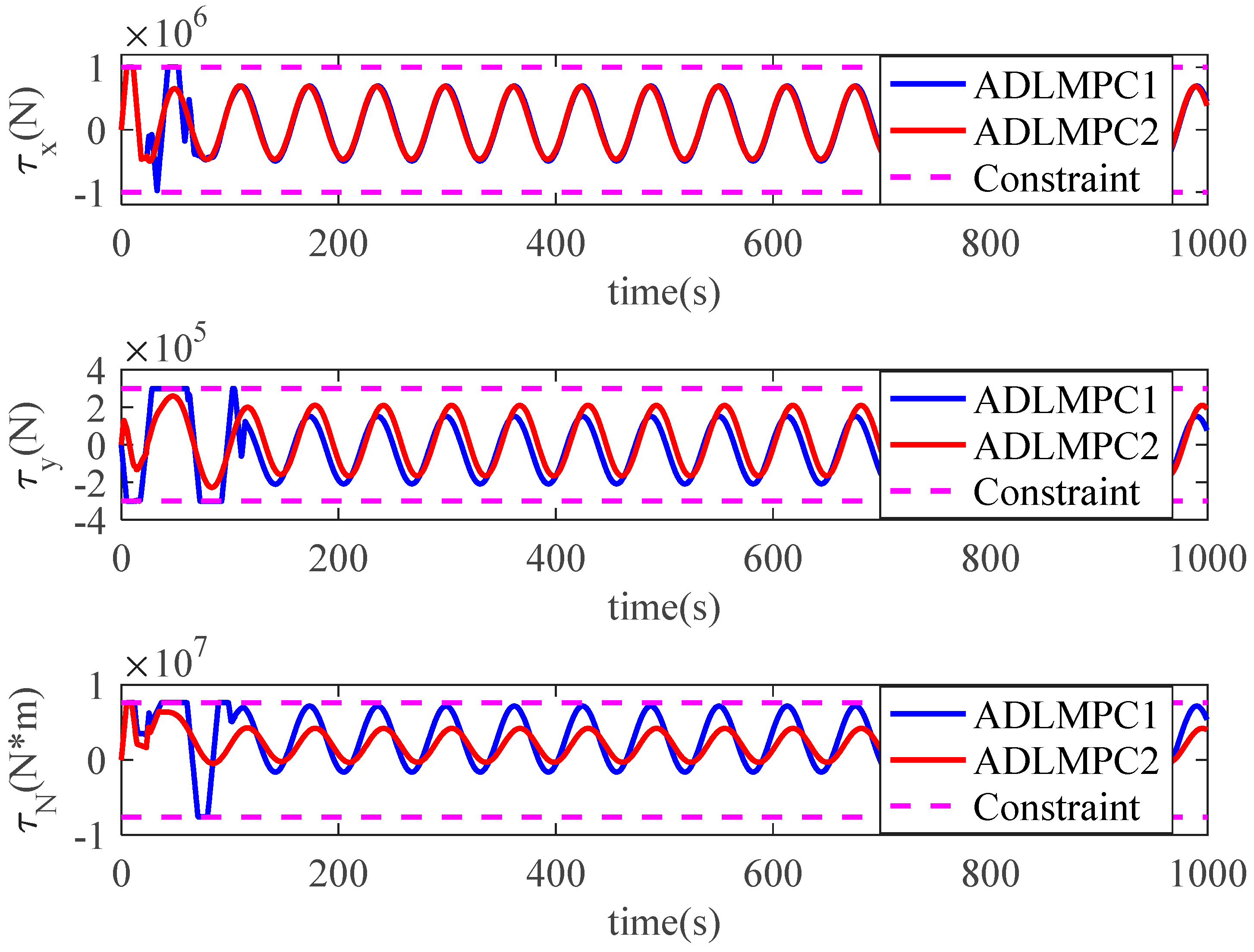
Figure 15. Control input generated by ADLMPC1 and ADLMPC2.

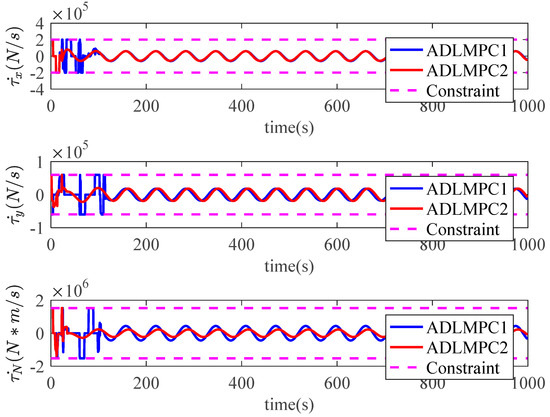
Figure 16. Rate of change in control input generated by ADLMPC1 and ADLMPC2.

The ship trajectories controlled by the ADLMPC1 controller and the ADLMPC2 controller are demonstrated in Figure 11, Figure 12, Figure 13 and Figure 14. The ADLMPC1 controller shows a high accuracy in tracking performance under the effects of environmental disturbances, whereas the quality of tracking by the ADLMPC2 controller deteriorates. Specifically, Figure 13 and Figure 14 illustrate that instead of maintaining the ship position and speed on the reference values, all these states fluctuate near the reference values. On the other hand, Figure 15 and Figure 16 show whether the magnitude of control inputs or rate of change in control inputs generated by the ADLMPC2 controller are smaller than those generated by the ADLMPC1 controller, especially in the first 100 s. The main reason for the phenomena above is that the values of elements in Q₁ are larger than those in Q₂, while the values of elements in R₁ are smaller than those in R₂. A decrease in Q and an increase in R mean that we pay more attention to the energy cost of thrusters rather than the accuracy in tracking. Therefore, the ADLMPC controller reduces the energy cost by degrading the tracking performance.

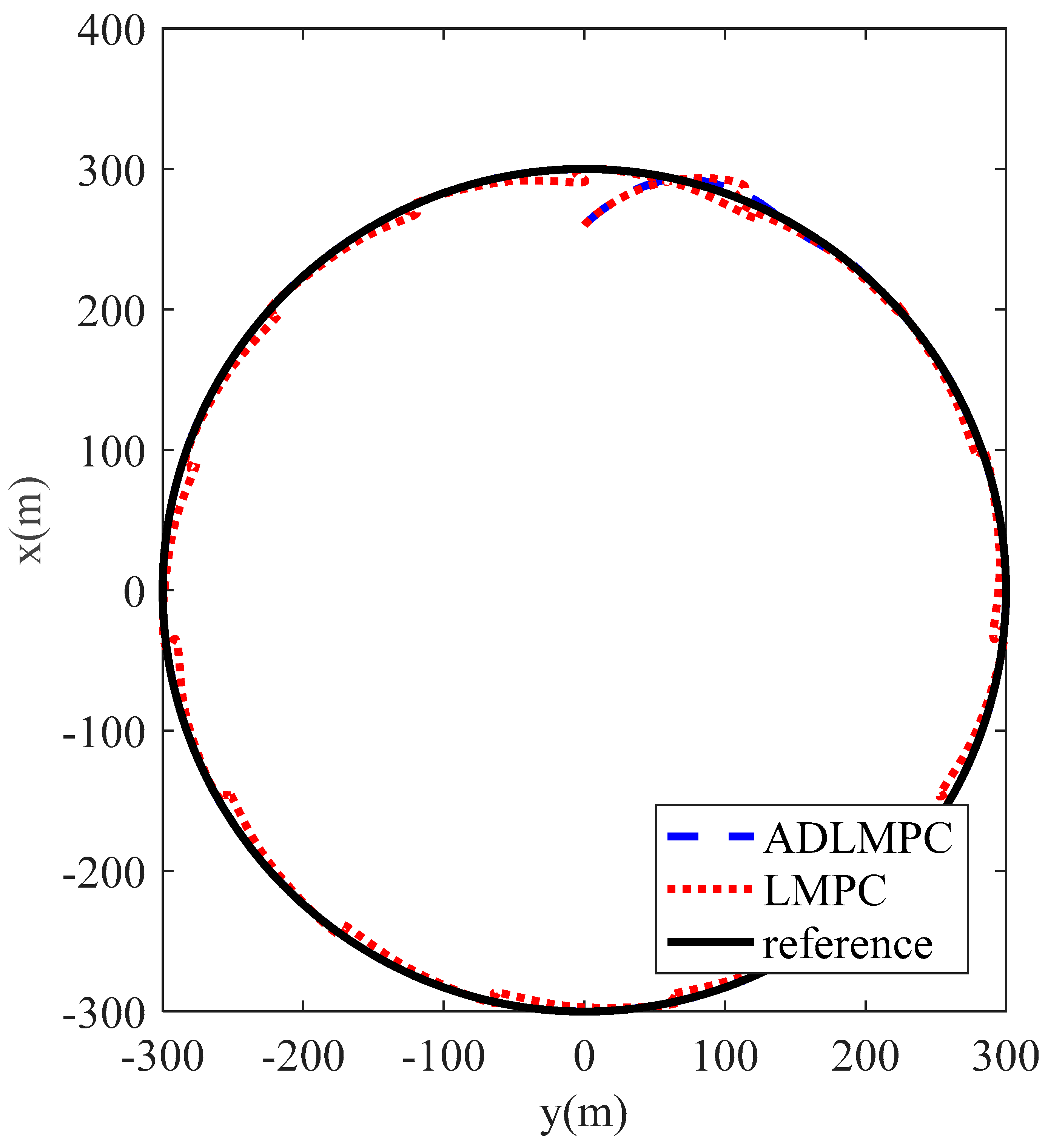
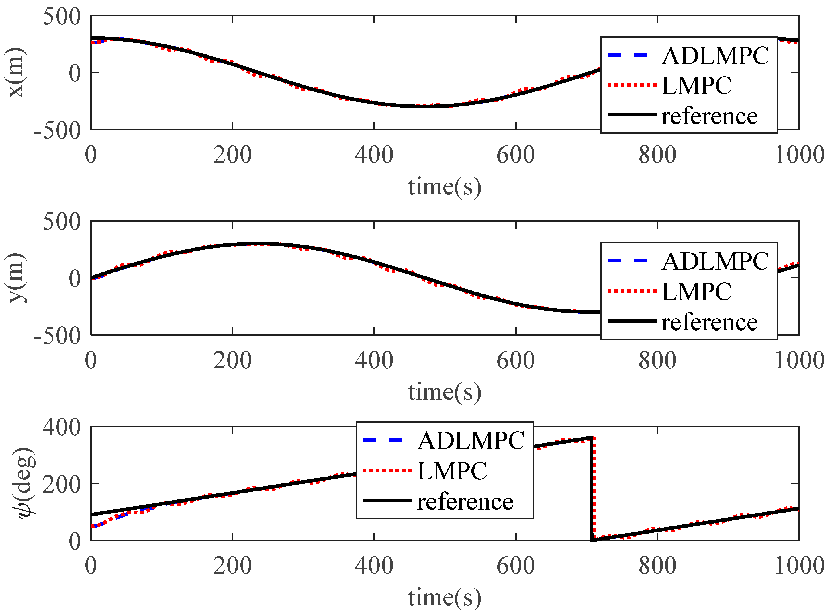
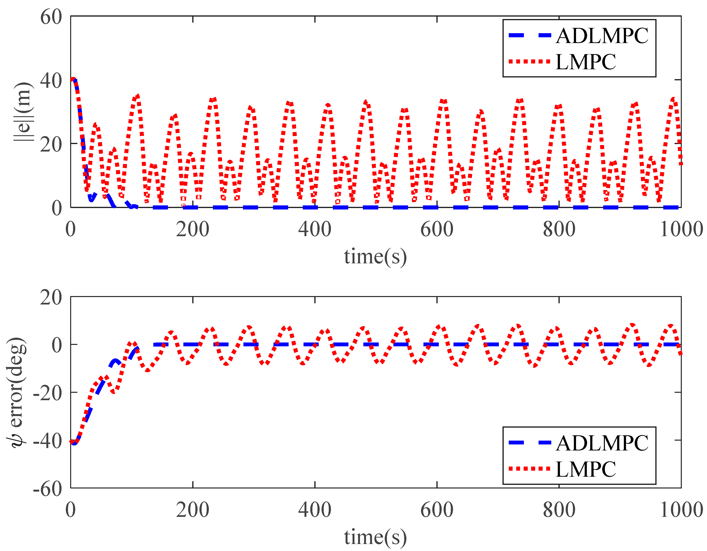
To investigate the advantage of anti-disturbance in the ADLMPC controller compared with the LMPC controller proposed in [25,26], we conduct the simulation (simulation case 3) under environmental disturbances. For effective comparison, the parameters for the LMPC controller and ADLMPC controller are set to the same values as those of the ADLMPC controller in case 1. The initial states of the model ship and environmental disturbances are also the same as those in case 1. Simulation results are shown in Figure 17, Figure 18 and Figure 19. These figures demonstrate that the accuracy of trajectory tracking in the effects of environmental disturbances in the ADLMPC controller is much higher than that of the LMPC controller. It can be seen from Table 2 that the MSEs of x, y, and ψ with the LMPC controller are more than 8 times, 20 times, and 10 times larger than those with the ADLMPC controller. These simulation results can illustrate the effectiveness of anti-disturbance with the ADLMPC controller.

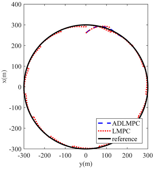
Figure 17. The trajectory of the DP ship controlled by ADLMPC and LMPC.

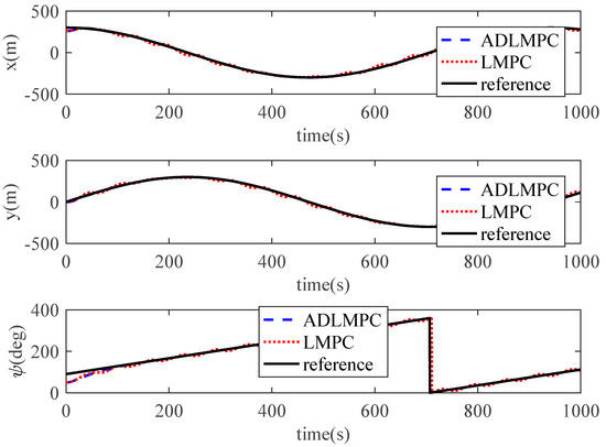
Figure 18. Position and heading variations of the DP ship controlled by ADLMPC and LMPC.

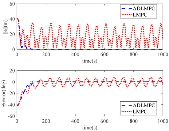
Figure 19. Tracking errors of position and heading controlled by ADLMPC and LMPC.

Table 2. Mean square errors of position states and heading state for case 3.

MSE	ADLMPC	LMPC	Improvement
x (m2)	23.9584	189.35	87.3%
y (m2)	4.1882	190.866	97.8%
ψ (rad2)	0.0174	0.1807	90.4%

5. Conclusions

In this paper, a novel ADLMPC scheme of low-speed trajectory tracking is proposed. With unknown environmental disturbances, the proposed ADLMPC scheme can accurately control the DP ship affected by constraints of control inputs and speed states to track reference trajectory optimally. By incorporating a tuned ESO to estimate disturbances, the estimations are exploited to update the predictive model in ADLMPC such that the control law generated by the ADLMPC controller can compensate for disturbances without violating control input constraints. A Lyapunov-based virtual control law that fulfills the requirements of the control inputs is designed and employed to establish the additional Lyapunov contraction constraint in ADLMPC, which naturally guarantees the recursive feasibility of ADLMPC and closed-loop stability. Furthermore, the range of parameters for the ADLMPC controller is wider than that of the LMPC controller proposed in [25,26], which means that the ADLMPC controller can control the DP ship to track reference trajectory more flexibly. Simulation results showed that, compared with the virtual controller combined with ESO and LMPC controller without ESO, the proposed ADLMPC control scheme could improve the accuracy of trajectory tracking and convergence time to reference trajectory under disturbances and constraints. The improvements in MSEs in position states with the virtual controller and LMPC controller are 20.2%, 73.5%, 0, and 87.3%, 97.8%, and 90.4%, respectively.

In the near future, the ship model test will be conducted to verify the proposed ADLMPC method. Furthermore, we notice that the current computing burden of the proposed ADLMPC is acceptable due to the optimization control problem and corresponding constraints being relatively simple in low-speed mode. When the DP ship navigates at high speed, this controlled system is underactuated and presents strong coupling and nonlinearity. In this situation, whether the real-time capability of ADLMPC can be guaranteed or not is unknown. Therefore, the extension of this work will focus on the implementation of ADLMPC on the trajectory tracking of the DP ship at high speed.

References

- Bian, X.Q.; Fu, M.Y.; Wang, Y.H. The Dynamic Positioning of The Ship, 1st ed.; Science Press: Beijing, China, 2011; pp. 5–9. [Google Scholar]
- Fossen, T.I.; Grovlen, A. Nonlinear Output Feedback Control of Dynamically Positioned Ships Using Vectorial Observer Back-Stepping. IEEE Trans. Control. Syst. Technol. 1998, 6, 121–128. [Google Scholar] [CrossRef]
- Wang, N.; Liu, Z.Z.; Zheng, Z.J.; Er, M.J. Global Exponential Trajectory Tracking Control of Underactuated Surface Vehicles Using Dynamic Surface Control Approach. In Proceedings of the 2018 International Conference on Intelligent Autonomous Systems, Singapore, Singapore, 1–3 March 2018. [Google Scholar]
- Vu, M.T.; Le, T.-H.; Thanh, H.L.N.N.; Huynh, T.-T.; Van, M.; Hoang, Q.-D.; Do, T.D. Robust Position Control of an Over-actuated Underwater Vehicle under Model Uncertainties and Ocean Current Effects Using Dynamic Sliding Mode Surface and Optimal Allocation Control. Sensors 2021, 21, 747. [Google Scholar] [CrossRef] [PubMed]
- Vu, M.T.; Thanh, H.L.N.N.; Huynh, T.-T.; Le Thanh, H.N.N.; Huynh, T.-T.; Thang, Q.; Duc, T.; Hoang, Q.-D.; Le, T.-H. Station-Keeping Control of a Hovering Over-Actuated Autonomous Underwater Vehicle Under Ocean Current Effects and Model Uncertainties in Horizontal Plane. IEEE Access 2021, 9, 6855–6867. [Google Scholar] [CrossRef]
- Yang, Y.; Du, J.L.; Guo, C.; Li, G. Trajectory tracking control of nonlinear full actuated ship with disturbances. In Proceedings of the 2011 International Conference of Soft Computing and Pattern Recognition, Dalian, China, 14–16 October 2011. [Google Scholar]
- Shen, Z.P.; Zhang, X.L.; Zhang, N. Recursive sliding mode dynamic surface output feedback control for ship trajectory tracking based on neural network observer. Control. Theory Appl. 2018, 35, 1092–1100. [Google Scholar]
- Fu, M.Y.; Xu, Y.J.; Zhou, L. Bio-inspired trajectory tracking algorithm for Dynamic Positioning ship with system uncertainties. In Proceedings of the 2016 Chinese Control Conference, Chengdu, China, 27–29 July 2016. [Google Scholar]
- Hu, C.D.; Wu, D.F.; Liao, Y.X.; Hu, X. Sliding mode control unified with the uncertainty and disturbance estimator for dynamically positioned vessels subjected to uncertainties and unknown disturbances. Appl. Ocean Res. 2021, 109, 102564. [Google Scholar] [CrossRef]
- Rojsiraphisal, T.; Mobayen, S.; Asad, J.H.; Vu, M.T.; Chang, A.; Puangmalai, J. Fast Terminal Sliding Control of Underactuated Robotic Systems Based on Disturbance Observer with Experimental Validation. Mathematics 2021, 9, 1935. [Google Scholar] [CrossRef]
- Thanh, H.L.N.N.; Vu, M.T.; Mung, N.X.; Nguyen, N.P.; Phuong, N.T. Perturbation Observer-Based Robust Control Using a Multiple Sliding Surfaces for Nonlinear Systems with Influences of Matched and Unmatched Uncertainties. Mathematics 2020, 8, 1371. [Google Scholar] [CrossRef]
- Wang, N.; Qian, C.J.; Sun, J.C.; Liu, Y.-C. Adaptive Robust Finite-Time Trajectory Tracking Control of Fully Actuated Marine Surface Vehicles. IEEE Trans. Control. Syst. Technol. 2016, 24, 1454–1462. [Google Scholar] [CrossRef]
- Wang, N.; Meng, J.E. Self-Constructing Adaptive Robust Fuzzy Neural Tracking Control of Surface Vehicles With Uncertainties and Unknown Disturbances. IEEE Trans. Control. Syst. Technol. 2015, 23, 991–1002. [Google Scholar] [CrossRef]
- Qiao, L.; Zhang, W.D. Adaptive non-singular integral terminal sliding mode tracking control for autonomous underwater vehicles. IET Control. Theory. Appl. 2017, 11, 1293–1306. [Google Scholar] [CrossRef]
- Alattas, K.A.; Mobayen, S.; Din, S.U.; Asad, J.H.; Fekih, A.; Assawinchaichote, W.; Vu, M.T. Design of a Non-Singular Adaptive Integral-Type Finite Time Tracking Control for Nonlinear Systems with External Disturbances. IEEE Access 2021, 9, 102091–102103. [Google Scholar] [CrossRef]
- Ghaffari, V.; Mobayen, S.; Din, S.U.; Rojsiraphisal, T.; Vu, M.T. Robust Tracking Composite Nonlinear Feedback Controller Design for Time-delay Uncertain Systems in The Presence of Input Saturation. ISA Trans. 2022, 129 Pt B, 88–99. [Google Scholar] [CrossRef]
- Mayne, D.Q. Model predictive control: Recent developments and future promise. Automatica 2014, 50, 2967–2986. [Google Scholar] [CrossRef]
- Xi, Y.G. Predictive Control, 2nd ed.; National Defense Industry Press: Beijing, China, 2013; pp. 192–195. [Google Scholar]
- Zhan, D.Z.; Zheng, H.R.; Xu, W. Tracking Control of Autonomous Underwater Vehicles with Acoustic Localization and Extended Kalman Filter. Appl. Sci. 2021, 11, 8038. [Google Scholar] [CrossRef]
- Gan, W.Y.; Zhu, D.Q.; Hu, Z.; Shi, X.; Yang, L.; Chen, Y. Model Predictive Adaptive Constraint Tracking Control for Underwater Vehicles. IEEE Trans. Ind. Electron. 2020, 67, 7829–7840. [Google Scholar] [CrossRef]
- Liu, C.; Sun, T.; Hu, Q.Z. Synchronization Control of Dynamic Positioning Ships Using Model Predictive Control. J. Mar. Sci. Eng. 2021, 9, 1239. [Google Scholar] [CrossRef]
- Zheng, Y.; Liu, Z.L.; Liu, L.T. Robust MPC-Based Fault-Tolerant Control for Trajectory Tracking of Surface Vessel. IEEE Access 2018, 6, 14755–14763. [Google Scholar] [CrossRef]
- Mhaskar, P.; El-Farra, N.H.; Christofides, P.D. Stabilization of nonlinear systems with state and control constraints using Lyapunov-based predictive control. In Proceedings of the 2005 American Control Conference, Portland, OG, USA, 8–10 June 2005. [Google Scholar]
- Shen, C. Motion Control of Autonomous Underwater Vehicles Using Advanced Model Predictive Control Strategy. Ph.D. Thesis, University of Victoria, Victoria, VIC, Canada, 2018. [Google Scholar]
- Shen, C.; Shi, Y.; Buckham, B. Trajectory Tracking Control of an Autonomous Underwater Vehicle Using Lyapunov-Based Model Predictive Control. IEEE Trans. Ind. Electron. 2018, 65, 5796–5805. [Google Scholar] [CrossRef]
- Gong, P.; Yan, Z.P.; Zhang, W.; Tang, J. Lyapunov-based model predictive control trajectory tracking for an autonomous underwater vehicle with external disturbances. Ocean Eng. 2021, 232, 109010. [Google Scholar] [CrossRef]
- Saback, R.M.; Conceicao, A.G.S.; Santos, T.L.M.; Albiez, J.; Reis, M. Nonlinear Model Predictive Control Applied to an Autonomous Underwater Vehicle. IEEE J. Ocean Eng. 2020, 45, 799–812. [Google Scholar] [CrossRef]
- Xue, R.C.; Dai, L.; Huo, D.; Xia, Y. Robust Model Predictive Control with ESO for Quadrotor Trajectory Tracking with Disturbances. In Proceedings of the 2022 IEEE 17th International Conference on Control & Automation, Naples, Italy, 27–30 June 2022. [Google Scholar]
- Lv, T.; Yang, Y.H.; Chai, L. Extended State Observer based MPC for a Quadrotor Helicopter Subject to Wind Disturbances. In Proceedings of the 2019 Chinese Control Conference, Guangzhou, China, 27–30 July 2019. [Google Scholar]
- Sun, Z.Q.; Xia, Y.Q.; Dai, L.; Liu, K.; Ma, D. Disturbance Rejection MPC for Tracking of Wheeled Mobile Robot. IEEE ASME Trans. Mechatron. 2017, 22, 2576–2587. [Google Scholar] [CrossRef]
- Alamdari, S.H.; Karras, G.C.; Marantos, P.; Kyriakopoulos, K.J. A Robust Predictive Control Approach for Underwater Robotic Vehicles. IEEE Trans. Control. Syst. Technol. 2020, 28, 2352–2363. [Google Scholar] [CrossRef]
- Alamdari, S.H.; Nikou, A.; Dimarogonas, D.V. Robust Trajectory Tracking Control for Underactuated Autonomous Underwater Vehicles in Uncertain Environments. IEEE Trans. Autom. Sci. Eng. 2021, 18, 1288–1301. [Google Scholar] [CrossRef]
- Liu, J.K. Sliding Mode Control Design and Matlab Simulation: The Basic Theory and Design Method, 3rd ed.; Tsinghua University Press: Beijing, China, 2015; pp. 237–239. [Google Scholar]
- Du, J.L.; Hu, X.; Sun, Y.Q. Adaptive Robust Nonlinear Control Design for Course Tracking of Ships Subject to External Disturbances and Input Saturation. IEEE Trans. Syst. Manag. Cybern. Syst. 2020, 50, 193–202. [Google Scholar] [CrossRef]
- Fossen, T.I.; Sagatun, S.I.; Sørensen, A.J. Identification of dynamically positioned ships. Control Eng. Pract. 1996, 4, 369–376. [Google Scholar] [CrossRef]
- Andersson, J.A.E.; Gillis, J.; Horn, G.; Rawlings, J.B.; Diehl, M. CasADi: A software framework for nonlinear optimization and optimal control. Math. Prog. Comp. 2019, 11, 1–36. [Google Scholar] [CrossRef]
Disclaimer/Publisher’s Note: The statements, opinions and data contained in all publications are solely those of the individual author(s) and contributor(s) and not of MDPI and/or the editor(s). MDPI and/or the editor(s) disclaim responsibility for any injury to people or property resulting from any ideas, methods, instructions or products referred to in the content. |
© 2023 by the authors. Licensee MDPI, Basel, Switzerland. This article is an open access article distributed under the terms and conditions of the Creative Commons Attribution (CC BY) license (https://creativecommons.org/licenses/by/4.0/).