Comparative Study on Numerical Simulation of Wave-Current Nonlinear Interaction Based on Improved Mass Source Function

Abstract

In coastal waters, wave propagation is often affected by rivers and tides. The wave current interaction increases the complexity of the wave propagation. In this study, we consider the Boussinesq type equation with an improved dispersion term as the governing equation and establish a numerical model of wave propagation in the coexistence of wave current environment. Firstly, we use the MIKE 21 BW model to simulate the propagation of dual-frequency waves. The Navier–Stokes equation wave model is used to verify the results and the Fourier transform is used to analyze and discuss the dual-frequency waves. Our findings show that the numerical model established by the Boussinesq equation can better describe the nonlinear interaction between waves more accurately at a much higher computational efficiency compared with the Navier–Stokes equation wave model. In addition, we set the constant current source point in the wave numerical model and conduct the numerical simulation of waves in the current environment, by improving the mass source wave generation method. The numerical simulation of wave-current interactions between uniform and variable water depths is performed, thus demonstrating its capability to describe accurately the influence of water flow on wave propagation.

1. Introduction

Rayleigh observed the interaction between waves and currents in tides in 1911. Longuet-Higgins and Stewart [1,2] proposed the energy balance equation in the wave-current coexistence environment and put forward the concept of radiation stress for the first time. Because of the existence of radiation stress, the wave height decreases, and the wavelength increases in the same flow direction; in the reverse flow cases, the wave height increases and the wavelength decreases. This phenomenon was verified by Hughes and Stewart [3]. The wave height change subject to the action of current can be calculated theoretically by calculating the wave radiation stress [4]. Jonsson [5,6] summarized the wave propagation deformation subject to the action of current in physical experiments and considered the effect of wave on current in gentle slope terrain. Brevik and Bjørn [7,8] conducted physical model experiments during the encounter process of regular waves and uniform flow in rough and smooth terrain models, respectively. Li and Herbich [9] calculated and analyzed the changing trend of wave height and wavelength of Stokes wave theory subject to the action of currents. Compared with linear wave theory, nonlinear wave theory has a broader scope of application in the current environment. Swan et al. [10] conducted a physical model experiment of wave propagation in the current environment where the velocity is not uniformly distributed with the water depth. Lian and Zhao [11] started from the Navier–Stokes equation, introduced the flow equation and wave equation of the corresponding turbulence model to close the wave current coexistence field and solved the velocity distribution in the full depth when wave current coexistence occurs. Alfonsi et al. introduced the diffraction of water waves induced by a large-diameter, surface-piercing, vertical circular cylinder based on the Navier-Stokes equations [12]. Different nonhydrostatic models were proposed and developed by Dong et al. [13] and Ai et al. [14] to simulate the propagation of nonlinear wave trains. Based on the incident wave conditions, Ruffini et al. established a hydrological and morphological dynamic model of bichromatic wave groups in the middle beach [15].

Following improvement in the ability to conduct numerical calculations, scholars have increasingly performed numerical simulations of wave-current interaction. Thomas [16,17] established a numerical model of waves in the current environment to simulate numerically the propagation of linear and nonlinear waves subject to the action of currents. Wolf and Prandle [18], Sørensen et al. [19], Baschek [20], and Yan Yixin [21] studied the interaction between variable currents and waves and established a numerical model of the interactions between waves and tides. Li Yucheng and Zhang Yonggang [22]; Chen et al. [23]; Zou et al. [24]; Wang Yaling and Zhang Hongsheng [25]; Zhang Hongsheng et al. [26], based on the Boussinesq equation, introduced the flow velocity, proposed a new Boussinesq equation considering wave-current interaction, and established a nonlinear wave propagation numerical model subject to the action of non-uniform flow. Hong Guangwen et al. [27] proposed a wave propagation model for water depth and slowly varying waters based on the gentle slope equation and conducted a numerical simulation of wave deformation in the Yangtze River estuary. The results showed that the model has good practical engineering value. Wu Yongsheng et al. [28]; Liu Yingzhong Clock [29] and Teles et al. [30] used the Navier–Stokes equation as the control equation and conducted a numerical simulation of wave and current to study the interaction between wave and current. Li et al. successfully simulated the bichromatic wave based on the push-plate wave-making system [31].

To generate a traveling wave, the mass source wave-generating method is usually used. The principle of this method includes the addition of a source term to the governing equation in the specific region of the wave numerical model that contains the motion characteristics of water quality points during wave propagation. Adding the source term to the continuity equation for wave-making is commonly referred to as mass-source wave-making. By contrast, waveform generation by adding a source term to the continuity equation is called mass source waveform generation. Brorsen and Larsen [32] proposed the mass source wave-generating method based on the potential flow theory. The wave source could be placed at any location in the wave numerical model, and the wave simulation is conducted by controlling the flow density in the source region. Lin [33] developed and improved the mass source wave-generating method to make it applicable to various wave types. The wave source is set below the water surface and will not be disturbed by water surface fluctuations. Thus, the mass source wave-generating method will not be affected by the reflected wave. Wei et al. [34] introduced the mass source wave-generating method into the Boussinesq-type equation and used 1D and 2D wave numerical models to simulate single-frequency and random waves. Chen et al. conducted a numerical simulation of nonlinear wave propagation based on the mass source wave-making method of the stokes equation, but the calculation efficiency was low [35].

In addition, many scholars (Ha et al. [36]; Li et al. [37]; Gao et al. [38]; Wang et al. [39]; Ning et al. [40]) have introduced the mass source wave-generating method into different wave numerical models. This emphasizes the strong applicability and versatility of this method. Furthermore, since the mass source wave-making method has the advantage of not being affected by reflected waves, it becomes very suitable for numerical wave simulations of nearshore complex terrain (Gobbi and Kirby [41]).

Regarding the solution and application of the Boussinesq equation, Andrzej [42] developed some numerical methods to solve non-Hamiltonian integrable simplified turbulence equations, Mohapatra [43] proposed an internal wave analysis model in the presence of interfacial tension between a rigid floating plate and a rigid bottom part in a two-layer fluid setup and compared the results of long nonlinear internal waves in shallow water analysis and numerical wave model by using the Korteweg-de Vries equation, which has the same properties as those of the Boussinesq equation in the shallow-water traveling-wave solution [44]. Dinvay [45] simulated the surface wave of an inviscid incompressible fluid layer by improving the equation, which can be regarded as the weak nonlocal dispersion perturbation system of the shallow water system. In turn, Karaagac et al. [46] established a technique for simulating water-wave problems in weakly dispersive media (such as surface or ionic acoustic waves in shallow water). Additionally, Yao et al. [47] introduced the analysis of parametric effects in the wave profile of the variant Boussinesq equation through two analytical approaches. Fang [48] improved the Boussinesq model and described the permanent solitary wave solution and the numerical performance of the model in describing the solitary waves over complex bathymetries.

In this study, Madsen et al. [49,50] improved the Boussinesq equation of the dispersion term as the control equation and improved the mass-source wave-making method. Its application range is $\mu \le 0.5$ (or $kh\approx 3.1$, where $kh$ is the relative wave number). The MIKE 21 BW model, based on the Boussinesq equation, and the wave propagation model, based on the Navier–Stokes equation, are compared, and the wave propagation numerical model in the wave-current coexistence environment is established. The calculation efficiency of the MIKE 21 BW model is much higher than that of the Navier–Stokes equation model, and according to the improvement of Madsen et al. [51,52] and Sørensen et al. [53,54], the Boussinesq equation can describe the wave breaking and moving shoreline, thus paving the way for the study of the interactions between waves and structures at a subsequent stage.

2. Numerical Models

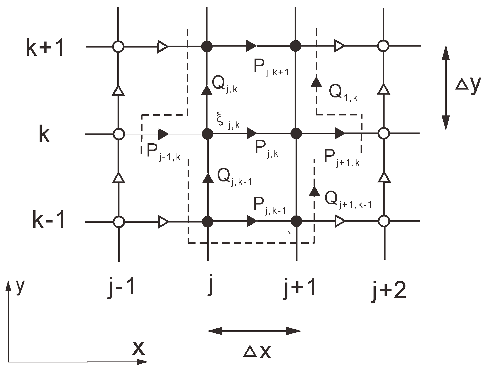
2.1. Control Equations and Solution Methods for the MIKE 21 BW Two-Dimensional Model

Continuity equation:

$$n\frac{\partial \eta }{\partial t}+\frac{\partial P}{\partial x}+\frac{\partial Q}{\partial y}=0$$

(1)

x-direction momentum equation:

$$\begin{array}{l}n\frac{\partial P}{\partial t}+\frac{\partial }{\partial x}\left(\frac{P^2}{d}\right)+\frac{\partial }{\partial y}\left(\frac{PQ}{d}\right)+\frac{\partial R_{xx}}{\partial x}+\frac{\partial R_{xy}}{\partial x}+F_x{n}^{2}gd\frac{\partial \eta }{\partial x}+\\ n^{2}P\left[\alpha +\beta \frac{\sqrt{P^2+Q^2}}{d}\right]+\frac{gP\sqrt{P^2+Q^2}}{d^2{C}^2}+n{\psi }_1=0\end{array}$$

(2)

y-direction momentum equation:

$$\begin{array}{l}n\frac{\partial Q}{\partial t}+\frac{\partial }{\partial y}\left(\frac{Q^2}{d}\right)+\frac{\partial }{\partial x}\left(\frac{PQ}{d}\right)+\frac{\partial R_{xx}}{\partial x}+\frac{\partial R_{xy}}{\partial x}+F_y{n}^{2}gd\frac{\partial \eta }{\partial y}+\\ n^{2}Q\left[\alpha +\beta \frac{\sqrt{P^2+Q^2}}{d}\right]+\frac{gP\sqrt{P^2+Q^2}}{h^2{C}^2}+n{\psi }_2=0\end{array}$$

(3)

where Boussinesq dispersion terms ${\psi }_1$ and ${\psi }_2$ are derived using the slow-varying water depth assumption of Madsen and Sørensen [49].

$$\begin{gathered} {\psi }_1=-\left(B+\frac{1}{3}\right)h^2\left(P_{xxt}+Q_{xyt}\right)-nBg{h}^3\left({\eta }_{xxx}+{\eta }_{xyy}\right) \\ -h{h}_x\left(\frac{1}{3}{P}_{xt}+\frac{1}{6}{Q}_{yt}+nBgh\left(2{\eta }_{xx}+{\eta }_{yy}\right)\right)-h{h}_y\left(\frac{1}{6}{Q}_{xt}+nBgh{\eta }_{xy}\right) \end{gathered}$$

(4)

$$\begin{gathered} {\psi }_2=-\left(B+\frac{1}{3}\right)h^2\left(Q_{yyt}+P_{xyt}\right)-nBg{h}^3\left({\eta }_{yyy}+{\eta }_{xxy}\right) \\ -h{h}_y\left(\frac{1}{3}{Q}_{yt}+\frac{1}{6}{P}_{xt}+nBgh\left(2{\eta }_{yy}+{\eta }_{xx}\right)\right)-h{h}_x\left(\frac{1}{6}{P}_{yt}+nBgh{\eta }_{xy}\right) \end{gathered}$$

(5)

where $\eta$ denotes the free-surface displacement, P and Q denote the cross-sectional flows in the x- and y-directions, respectively, $B$ denotes Boussinesq dispersion coefficient (when $B=1/15$ it can better reflect the dispersion characteristics of waves [42]); $F_x$ and $F_y$ denote the horizontal stress term in the x- and y-directions, respectively; $d$ denotes the total water depth; $h$ is the static water depth; n denotes the porosity; $C$ is the Chezy drag coefficient; $\alpha$ denotes the laminar drag coefficient in porous media, and $\beta$ denotes the turbulent drag coefficient in porous media.

The horizontal stress term in the equation can be derived from the gradient stress relationship as follows.

$$F_x=-\left\{\frac{\partial }{\partial x}\left(v_t\frac{\partial P}{\partial x}\right)+\frac{\partial }{\partial y}\left[v_t\left(\frac{\partial P}{\partial y}+\frac{\partial Q}{\partial x}\right)\right]\right\}$$

(6)

$$F_y=-\left\{\frac{\partial }{\partial y}\left(v_t\frac{\partial Q}{\partial y}\right)+\frac{\partial }{\partial x}\left[v_t\left(\frac{\partial Q}{\partial x}+\frac{\partial P}{\partial y}\right)\right]\right\}$$

(7)

where, $v_t$ is the vortex viscosity in the horizontal direction.

Solution method: The 2D model of MIKE 21 BW is discretized with a rectangular staggered grid, as shown in Figure 1. Scalar quantities, such as water surface elevation, are defined at the nodes of the grid, whereas the flow components in the corresponding directions are defined at the midpoints of the nodes’ connecting lines. The spatial derivative terms, other than the convective ones, are different centrally. The difference in time is in a central implicit format. The method uses a non-iterative alternating direction implicit (ADI) algorithm. The equations are discretized into the form of a tri-diagonal system of equations, for which the Double Sweep (DS) algorithm is used to solve.

2.2. Numerical Model and Solution of the Navier–Stokes Equation

The control equation uses the Navier–Stokes equation for incompressible fluids with velocity and pressure as variables.

Continuity equation:

$$\rho \left(\frac{\partial u}{\partial x}+\frac{\partial w}{\partial z}\right)=S_m$$

(8)

Momentum equation:

$$\rho \left(\frac{\partial u}{\partial t}+u\frac{\partial u}{\partial x}+w\frac{\partial u}{\partial z}\right)=-\frac{\partial p}{\partial x}+\mu \left(\frac{{\partial }^{2}u}{\partial x^2}+\frac{{\partial }^{2}u}{\partial z^2}\right)+S_x$$

(9)

$$\rho \left(\frac{\partial w}{\partial t}+u\frac{\partial w}{\partial x}+w\frac{\partial w}{\partial z}\right)=\rho g-\frac{\partial p}{\partial x}+\mu \left(\frac{{\partial }^{2}w}{\partial x^2}+\frac{{\partial }^{2}w}{\partial z^2}\right)+S_z.$$

(10)

where $\rho$ is the fluid density; $u$ is the x-direction velocity component; $w$ is the z-direction velocity component; $p$ is the pressure; $\mu$ is the dynamic viscosity coefficient; $S_m$ is the additional mass source term; $S_x$ is the x-direction additional momentum source term; $S_z$ is the z-direction additional momentum source term.

The VOF method is used to track the location of the free fluid surface. This method is currently a desirable treatment for problems with complex free surfaces. Defining ${\alpha }_q$ as the volume fraction occupied by the $q$ phase fluid in a cell, $q$ is taken as 1 or 2. Here, phase 1 is set to be air and phase 2 to be water.

• ${\alpha }_q$ has the following three values:
• ${\alpha }_q=0$: No phase $q$ fluid in the unit.
• ${\alpha }_q=1$: The unit is filled with phase $q$ fluid.
• $0<{\alpha }_q<1$: This unit is the intersection of phase $q$ liquid and other liquids.

Thus, for incompressible viscous fluids, the continuity equation for phase $q$ liquids:

$$\frac{\partial {\alpha }_q}{\partial t}+\frac{\partial \left(u{\alpha }_q\right)}{\partial x}+\frac{\partial \left(w{\alpha }_q\right)}{\partial z}=0 q=1,2$$

(11)

and

$${\displaystyle \sum _{q=1}^2{\alpha }_q}=1$$

(12)

Solution method:The software FLUENT uses the finite volume method to numerically solve the Navier–Stokes equation in the case of incompressible fluids. The finite volume method was used here, and the basic idea was to divide the computational region into a series of control volumes, where the nodes between the control volumes constituted the grid points. The ultimate goal was to determine the values of the variables at each grid point. The partial differential equation was integrated into the control volume to discretize the equation. An interpolation function was introduced between the grid points to calculate the integral of the control volume. Different interpolation functions can be used for different terms of the same equation. The discrete equations of the finite volume method have conservation properties in the control volume and can be directly physically interpreted. Therefore, the finite volume method has a more significant advantage in the numerical simulation of fluids.

The separation solution method is often used for the numerical simulation of low-speed flows with weak mutual dependence on density, power, energy, etc. Therefore, for the numerical simulation of waves, the separation solution method of pressure correction was adopted. It includes the solution of the variable separation in the control equation separately and the execution of multiple iterations of the discrete equation to prevent the results from being divergent. The multiple iteration solving of equations in these cases imposes the need for a higher memory compared to the case of the coupled method. Pressure correction means that the solved equation includes a pressure correction equation, derived from the continuity equation. In each time-step operation, the initial pressure field was assumed first, and the velocity field was solved accordingly. Then the pressure correction equation was solved, correcting both the pressure and velocity fields. In this manner, the convergence solution between the pressure and velocity fields was solved.

Secondary development: The numerical modeling of wave propagation using

FLUENT requires the use of its secondary development function in both the wave creation and wave extinction sections. User-defined functions (UDFs) were added to the wave propagation model to achieve specific purposes. This wave model uses the

DEFINE_SOURCE macro to implement the secondary development of FLUENT, which defines $S_m$, $S_x$, and $S_z$ in the control equations. This improves the original control equations and enables the source term wave generation and dissipation.

3. Research Methods

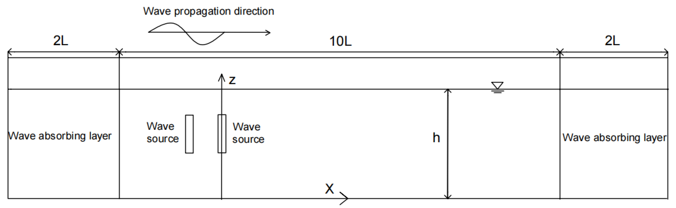
3.1. Mass Source Wave-Generation Method

The mass source wave generation method is only applicable to the numerical model of waves. Its principle is to add the wave generation source term function to the continuity equation and generate various wave patterns through different source term functions. The wave source is set in the model water area and can be either a point, line, or finite volume source (MIKE 21 BW model uses a line source whereas the Navier–Stokes equation wave model uses a finite volume source). This wave source is equivalent to a source-sink point with changing intensity. In the wave numerical model, it is necessary to set a wave elimination zone in the opposite direction of the wave propagation to eliminate the influence of reflected waves. See Figure 2 for details.

3.2. Single-Frequency Waveform Generation

The controlling equation in the wave-making region Ω is given by:

$$\rho \left(\frac{\partial u}{\partial x}+\frac{\partial w}{\partial z}\right)=S_m\left(t\right),$$

(13)

where $S_m\left(t\right)$ is the time-dependent mass source term function.

The wavefront equation for a single-frequency wave is:

$$\eta \left(x,t\right)=\frac{H}{2}\cos \left(kx-\omega t\right)$$

(14)

In the wave area $\mathsf{\Omega }$, the value $x=x_0$, where $x_0$ is the central point horizontal coordinate of the wave area $\mathsf{\Omega }$. If the mass source is a point or the source, $x_0$ is the horizontal coordinate of the mass source. The mass source term function and wave surface equation satisfy:

$${\displaystyle {\int }_0^t{\displaystyle {\int }_{\mathsf{\Omega }}{S}_m}}\left(t\right)d\mathsf{\Omega }dt=2\rho {\displaystyle {\int }_0^{t}C\eta \left(x_0,t\right)}dt$$

(15)

The integration yields:

$$S_m\left(t\right)=\frac{\rho CH}{A_{\mathsf{\Omega }}}\cos \left(\omega t\right),$$

(16)

where $C$ is the wave speed and $A_{\mathsf{\Omega }}$ is the total area of the grid covered by the wave-making region.

To ensure the stability of the calculation, the mass source function is written in the following form for the first three wave periods of the model calculation.

$$S_m\left(t\right)=\{\begin{array}{l}\frac{\rho CH}{A_{\mathsf{\Omega }}}\cos \left(\omega t\right)\left[1-\exp \left(-2.0t/T\right)\right]\\ \frac{\rho CH}{A_{\mathsf{\Omega }}}\cos \left(\omega t\right)\end{array}\begin{array}{l},t\le 3.0T\\ \\ ,others\end{array}$$

(17)

The position and size of the mass source wave has a significant influence on the wave-making effect. The width of the finite volume source should not exceed 5% of the effective wavelength. The height of the wave source shall be 1/5 to 1/4 of the water depth h, and the vertical distance from the center point of the wave source to the still water surface shall be 1/3 to 1/2 of the water depth h [32].

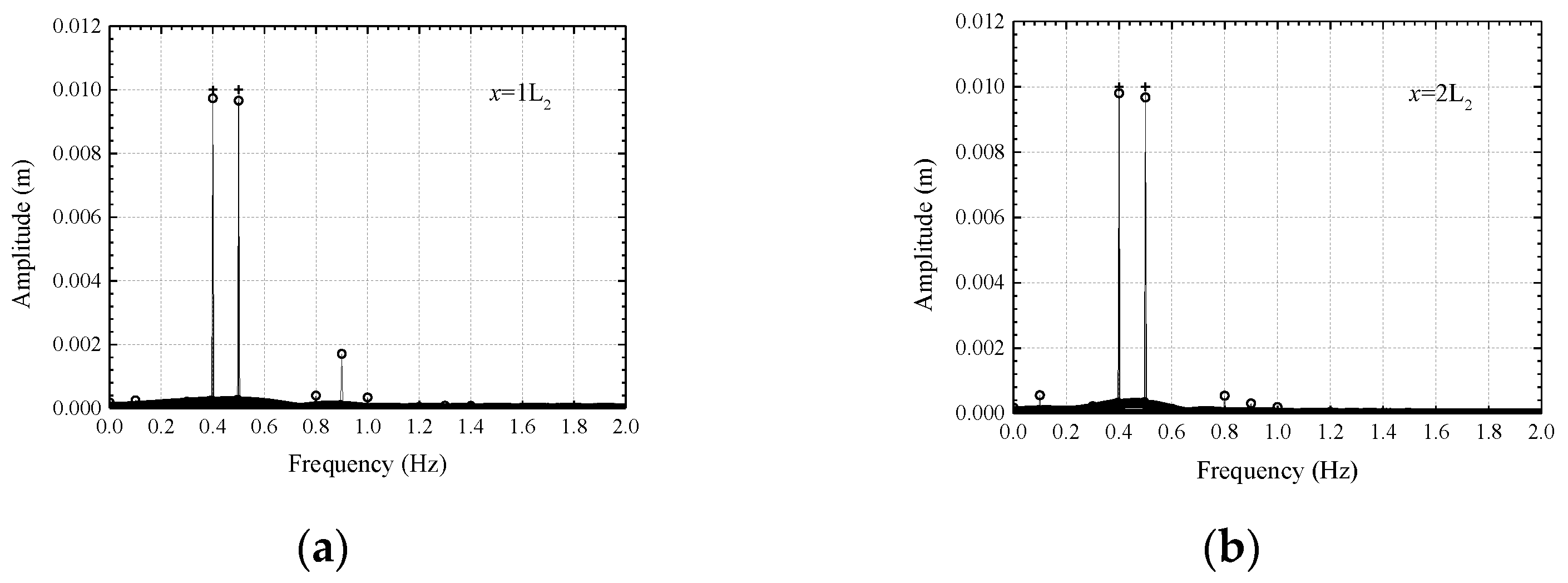
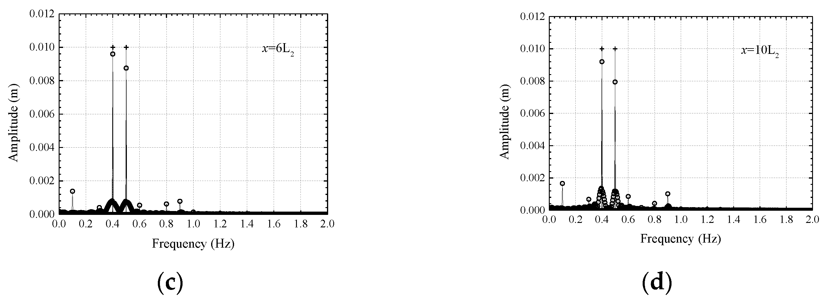
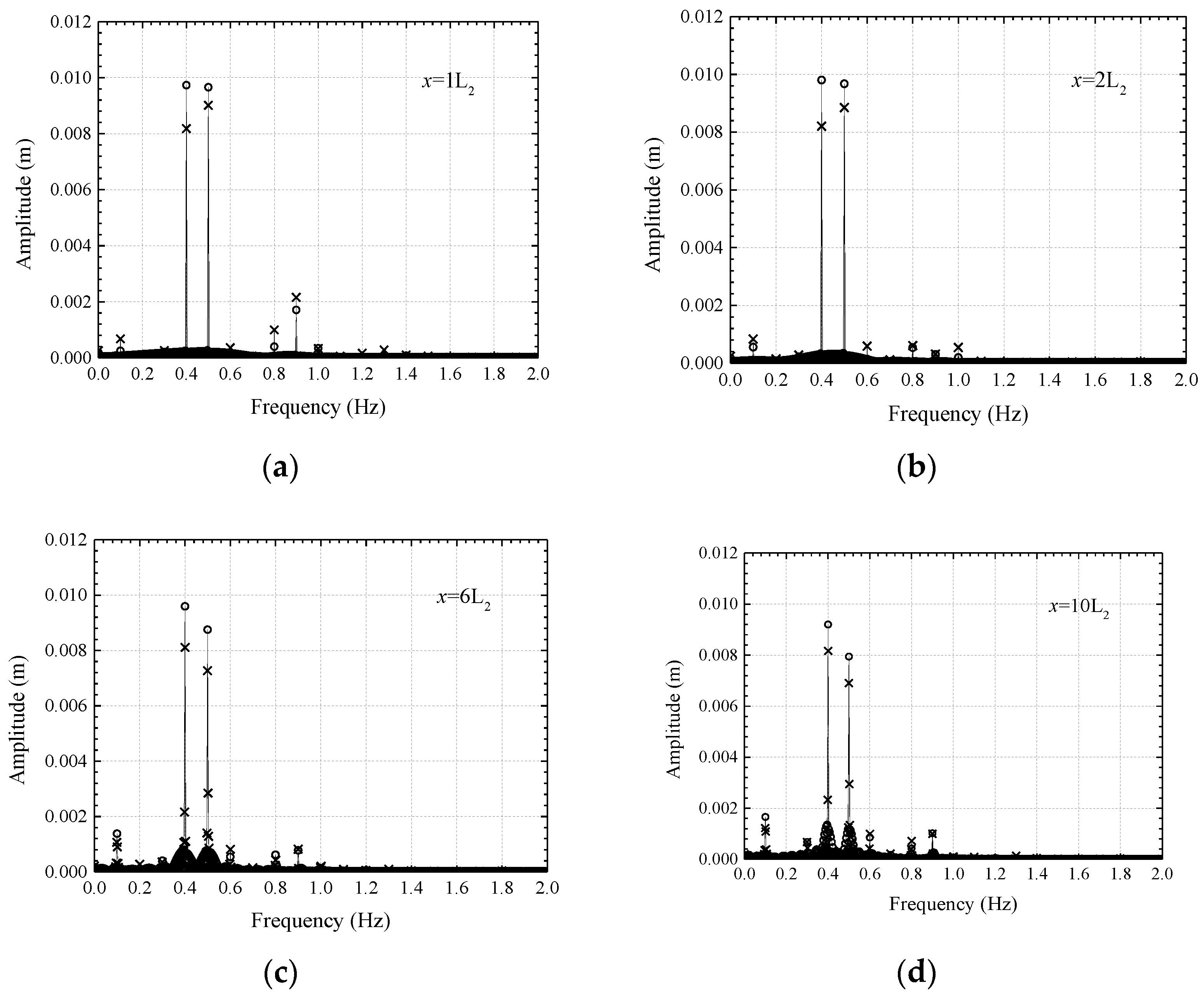
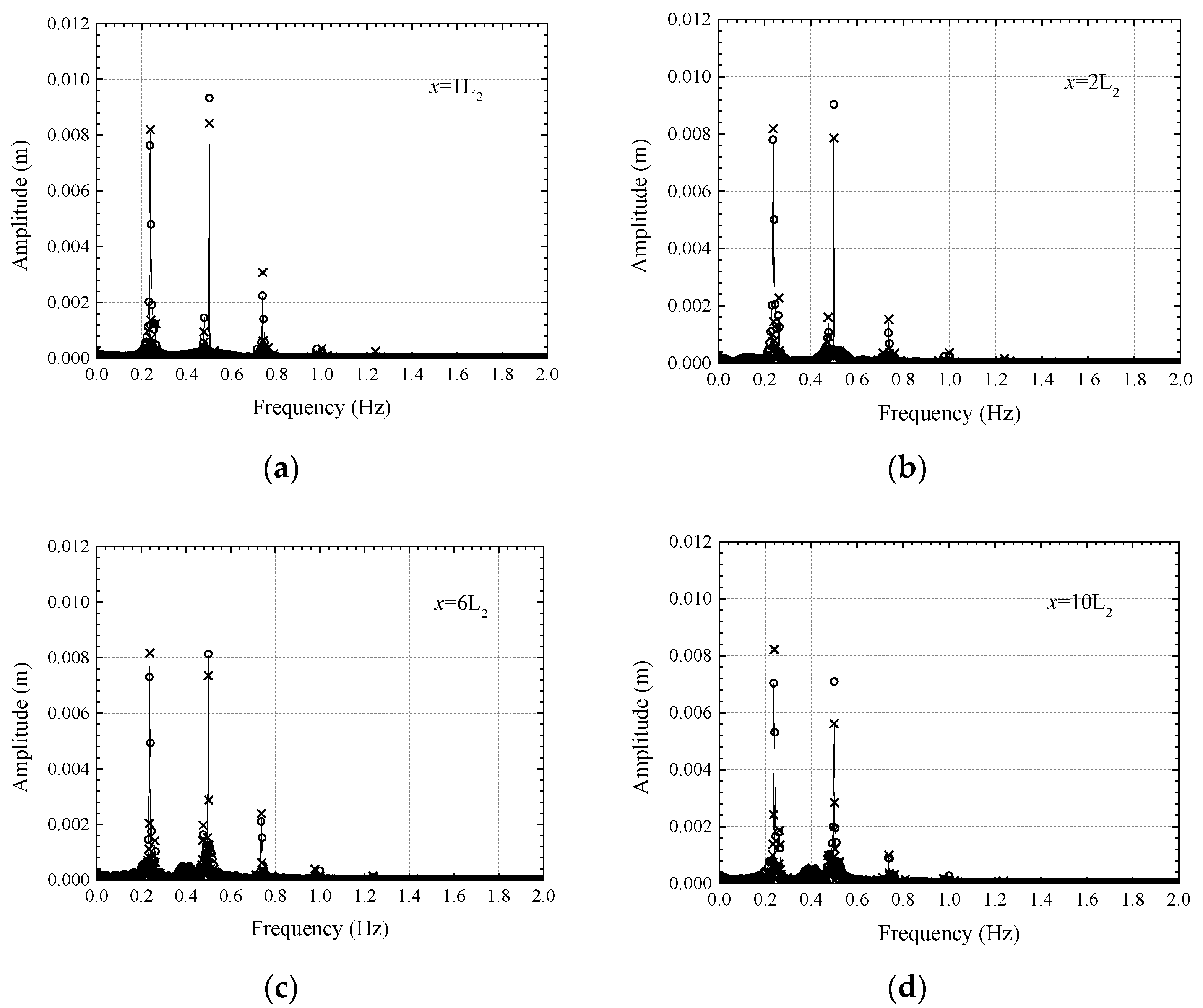
3.3. Interaction between Dual-Frequency Wave Generation and Wave-Current

The mass source wave generation method has the advantage of not being affected by the reflected wave or by other wave sources. Therefore, the mass source wave generation method is used for the numerical simulation of dual-frequency waves, where two wave sources are set in the wave numerical model. Their intensities do not mutually affect each other, whereas the interaction of the two columns of waves is represented in the rest of the calculated water (Figure 2) The horizontal distance between the centers of the two sources is considered five times the water depth h.

The mass source wave generation method is also naturally applicable to the numerical simulation of wave flow interaction. According to the formula, the mass source term function of the wave can be changed to the water flow mass source term function:

$$S_m\left(t\right)=\frac{2\rho U_c\left(t\right)}{A_{\mathsf{\Omega }}},$$

(18)

where $U_c\left(t\right)$ is the velocity function of the water flow.

The current source term is set at both ends of the wave model to obtain a stable current in the wave propagation numerical model. The wave source term is set between the two current source terms to establish the wave propagation model in the stable current and numerically simulate the propagation and deformation of waves in the current environment.

3.4. Numerical Wave Elimination Methods

In the numerical simulation of waves, the wave elimination treatment should be conducted at the boundary of the model. The wave-absorbing layer can absorb the excess wave energy, eliminate the influence of the reflected wave on the calculation results, and prevent the calculation divergence. The principle based on which the wave-absorbing layer simulated involves the addition of a damping coefficient to the variable of the wave numerical model. The value of the variable will thus decay during the wave propagation in the numerical solution, this achieves the purpose of numerical wave elimination. The artificial damping wave elimination area is set at the boundary of the numerical model. The wave elimination effect of the wave elimination layer is related to the width of the wave elimination layer, which is typically equal to 1–2 times its wavelength.

3.4.1. Numerical Extinction of the MIKE 21 BW Model

In the MIKE 21 BW model, the wave cancellation is achieved by using a damping coefficient in the variable about the x-partial differential in the type Boussinesq equation. In the fluctuation region, the variables $P$, $Q$ of the continuity equation and the variable $\eta$ of the momentum equation are multiplied by the damping coefficient $v\left(x\right)$:

$$v\left(x\right)=\alpha +\left(1-2\alpha \right)/\mu \left(x\right)+\alpha /{\mu }^2\left(x\right),$$

(19)

where $\mu \left(x\right)$ is the dissipation factor.

$$\mu \left(x\right)=\{\begin{array}{l}\exp \left[\left(2^{-x/\Delta x}-2^{-\left(x_{sr}-x_{sl}\right)/\Delta x}\right)\ln a\right]\\ 1\end{array}\begin{array}{l}{x}_{sl}\le x\le x_{sr}\\ x<x_{sr}\left(or\right)x>x_{sl}\end{array}$$

(20)

where $\alpha$ is the weighting factor, taken as 0.5; $\Delta x$ is the spatial step in the x-direction of the numerical wave model; $x_{sl}$ is the position of the beginning of the dissipation layer, $x_{sr}$ is the position of the end of the dissipation layer, the width of the dissipation layer is set to 1–2 times the wavelength; a is the dissipation factor at the end of the dissipation layer, taken as 10.

3.4.2. Numerical Wave Dissipation for the Navier–Stokes Equation Wave Model

In the Navier–Stokes equation wave model, wave cancellation is achieved by adding a cancellation source term to the momentum equation. The dissipation source term is as follows:

$$S_x=-\rho \xi \left(x\right)u$$

(21)

$$S_z=-\rho \xi \left(x\right)w$$

(22)

$$\xi \left(x\right)=\omega \frac{x-x_{sl}}{x_{sr}-x_{sl}}$$

(23)

where $\xi \left(x\right)$ denotes wave attenuation coefficient function; $\omega$ denotes frequency. Compared with the attenuation coefficient of the MIKE 21 BW model, the momentum source term of the Navier–Stokes equation wave model is simpler in form. When the width of the wave-absorbing layer is 1–2 times the wavelength, it also has a favorable wave-absorbing effect.

4. Numerical Simulation and Comparative Verification

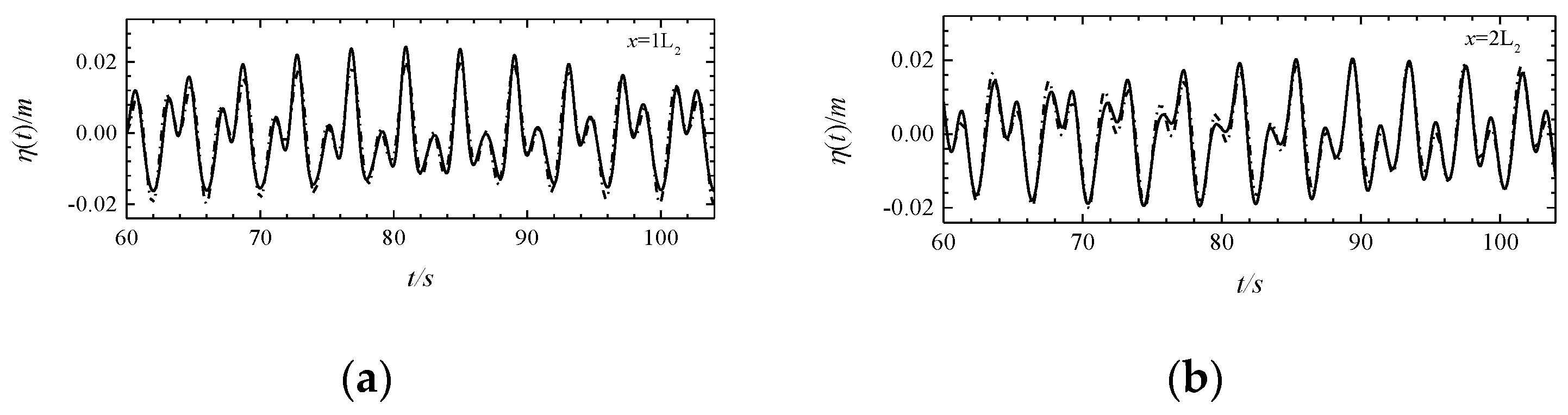
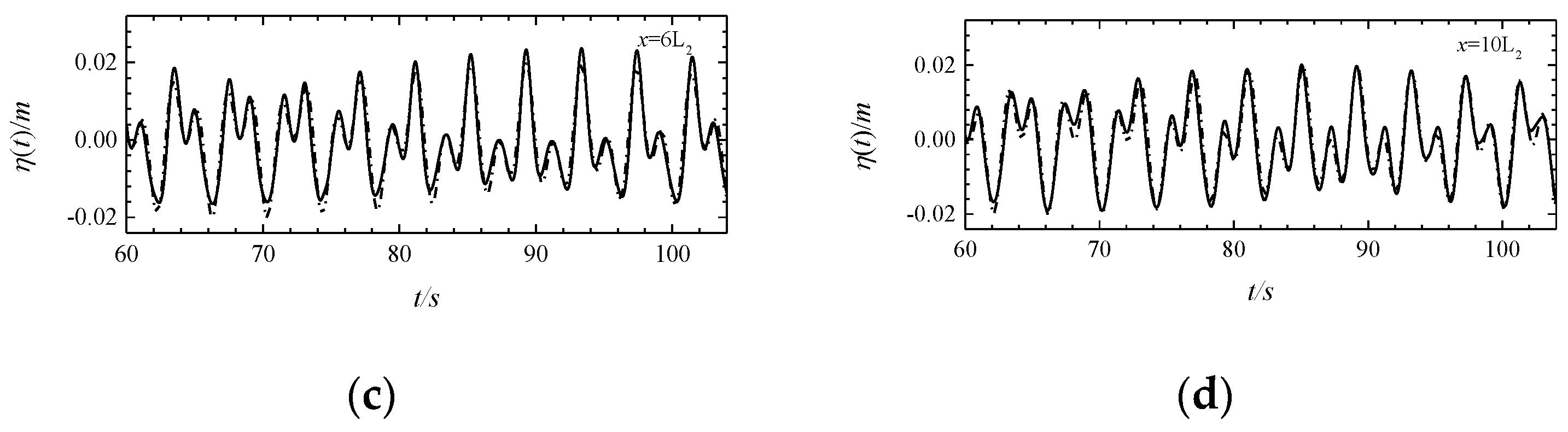
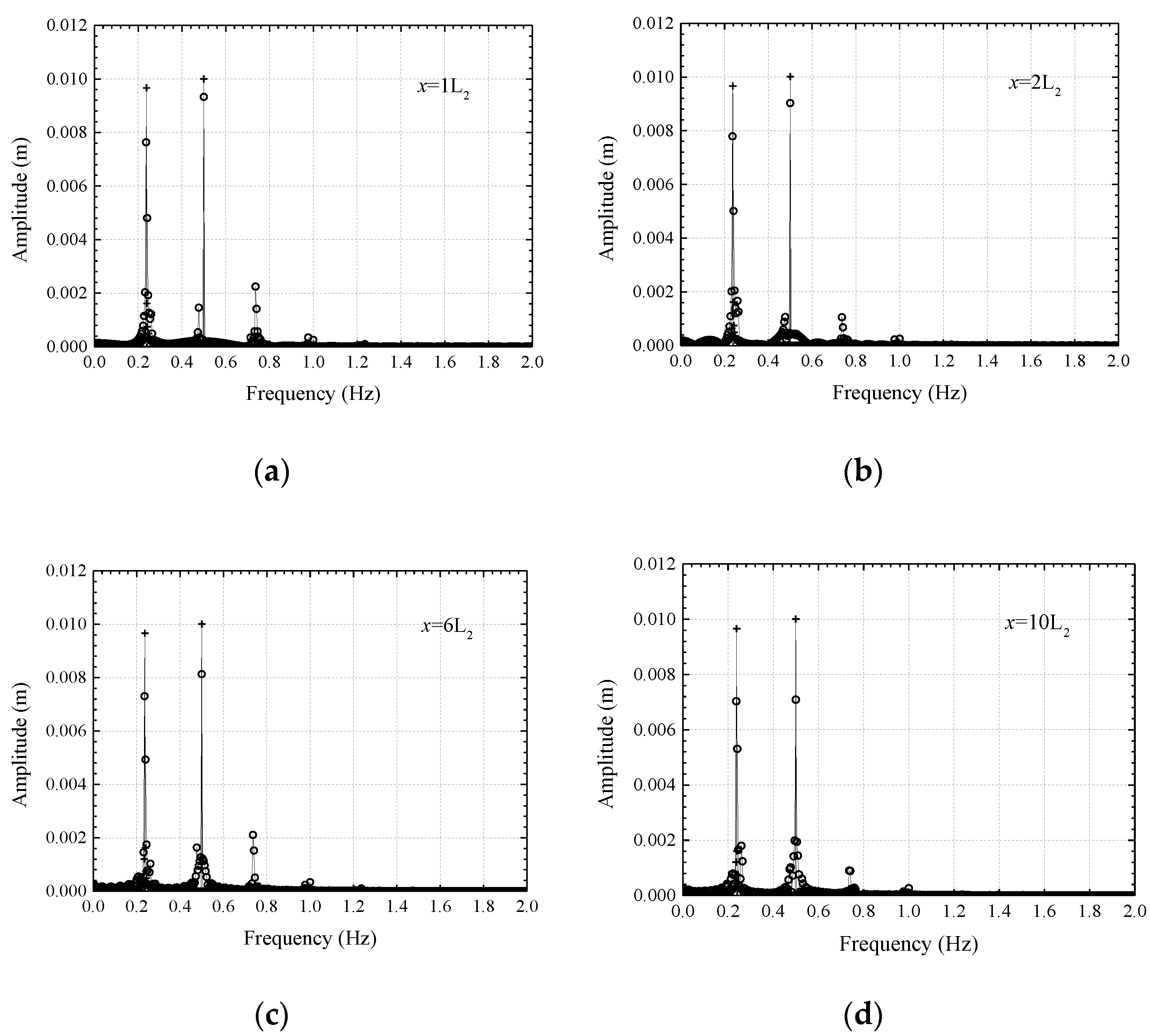
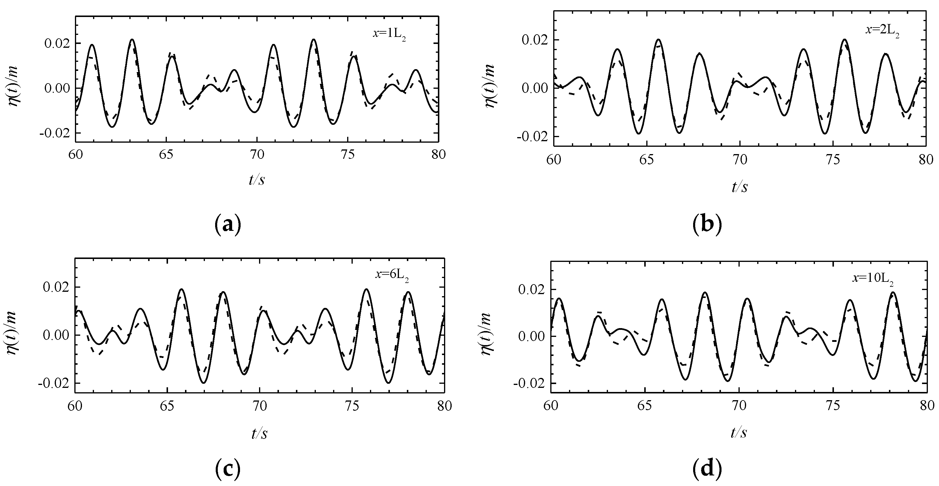
4.1. Wave-Wave Interactions

4.1.1. Numerical Extinction of the MIKE 21 BW Model

The periods of the simulated wave were set to 2.0 s, 2.5 s, 2.0 s, 4.2 s, respectively, and the amplitude is set to 0.01 m. The numerical sink length was set based on the maximum wavelength of the two waves. A uniform water depth flume with a length of 10 times the wavelength and a water depth of 0.45 m was set. The numerical models of the two wave-making methods adopt the same boundary conditions and grid size to compare and analyze the two numerical simulations results. The left, right, and bottom boundaries of the flume are all set as solid wall boundaries, whereas the top boundary is set as a pressure inlet. The grid size is taken as 0.08 m in the horizontal direction ($\Delta x$), 0.025 m in the vertical direction ($\Delta z$), and the time step was 0.01 s. The specific wave parameters are shown in conditions C1 and C2 in

Table 1. Simulated working conditions with two-color waves at a uniform water depth.

	Wave 1			Wave 2
	T1/s	L1/m	μ1	T2/s	L2/m	μ2
C1	2	3.88	0.12	2.5	5.00	0.090
C2	2	3.88	0.12	4.2	8.67	0.052

.

The frequencies of waves 1 and 2 are f₁ and f₂, respectively, and the nonlinear interaction between waves generates f₁ − f₂ subharmonic (differential frequency) and f₁ + f₂ superharmonic (sum frequency). The subharmonic wave and superharmonic wave also have wave interaction. The primary frequencies of spectral analysis are listed in

Table 2. Main frequencies of the C1 spectrum analysis under working conditions.

	f1	f2	2f1	2f2	f1 + f2	f1 + 2f2	2f1 + f2	2f1 + 2f2	f1 − f2	2f2 − f1	2f1 − f2	2f1 − 2f2
Frequency (Hz)	0.50	0.40	1.00	0.80	0.90	1.30	1.40	1.80	0.10	0.30	0.60	0.20

and

Table 3. Main frequencies of the C2 spectrum analysis under working conditions.

	f1	f2	2f1	2f2	f1 + f2	f1 + 2f2	2f1 + f2	2f1 + 2f2	f1 − f2	f1 − 2f2	2f1 − f2	2f1 − 2f2
Frequency (Hz)	0.50	0.24	1.00	0.48	0.74	0.98	1.24	1.48	0.26	0.02	0.76	0.52

.

As shown in Figure 3, wave surface attenuation exists in the mass source wave generation method. Similarly, when the wave propagates to the influence position far away from the wave source, the wave surface attenuation phenomenon is no longer obvious. It is challenging to analyze the nonlinear strength of the numerical results of dual-frequency waves only by comparing the time-domain changes of waves. The wave frequency domain diagram is used to analyze the nonlinear interaction of waves. Fourier analysis is a common method used to analyze these nonlinear characteristics. The frequency domain diagram of the waves is obtained via the Fourier analysis of the time-domain change data of wave surfaces at different positions (Figure 4).

It can be seen from Figure 3 that the amplitude of the mass source wave generation method at the harmonic frequency increases with an increase in the wave propagation distance. This changing trend is consistent with the principle of the wave-making method. The mass source wave generation method simulates the propagation of dual-frequency waves by directly setting two wave sources. The wave interaction is not complete at a distance from the wave source; thus, the amplitude of the second-order harmonic is not apparent. As the nonlinear interaction between waves increases with the propagation distance, the second-order harmonic and the third-order harmonic continue to grow.

Figure 3 and Figure 4 show the comparison of wave surface calculation results at different positions between the MIKE 21 BW model and the theoretical solution for the working condition C1. As shown in Figure 3, the numerical calculation results of the MIKE 21 BW model are consistent with the theoretical solution of dual-frequency waves. The model can simulate wave propagation in the coexistence environment of two trains of waves in a stable manner. Figure 4 shows that on the harmonic frequency of double frequency wave, the amplitude of the calculation result of the MIKE 21 BW model is much larger than the theoretical solution. The amplitude of the theoretical solution on the harmonic frequency cannot be easily distinguished. This is mainly because the theoretical solution of the dual-frequency wave is derived based on Stokes’ finite amplitude wave theory, and only contains the approximate, second-order solution. The nonlinearity of the theoretical solution of the dual-frequency wave is weak.

Figure 5 and Figure 6 show that the amplitude of the calculation result for the MIKE 21 BW model at the central frequency is significantly smaller than that of the theoretical solution at the corresponding frequency. From the perspective of wave energy conservation, the results are precise because the double-frequency wave numerically simulated by the Mike 21 BW model has strong nonlinearity. Subject to the nonlinear interaction between the two primary frequency waves, the wave energy is transferred from the central frequency wave to the harmonic wave, resulting in a reduction in the amplitude of the main frequency wave. The nonlinearity of the theoretical solution of dual-frequency waves is weak. The wave energy is mainly concentrated on the main frequency wave, whereas the harmonic amplitude is always tiny. Compared with the theoretical solution of wave interaction, the Mike 21 BW model can better describe the nonlinear interaction between waves and has a sound engineering application prospect.

4.1.2. Comparison of the MIKE21 BW and Navier–Stokes Models

According to the numerical double frequency wave-generation method of the Navier–Stokes equation wave model, the calculated results of the Navier–Stokes equation wave model based on FLUENT software were selected to verify the double frequency wave simulation of the Boussinesq equation model. Both Navier–Stokes equation wave model and Mike 21 BW model adopt the mass source wave generation method. Figure 7, Figure 8, Figure 9 and Figure 10 are the results of the double-frequency wave numerical simulations of working conditions C1 and C2. The boundaries on the left, right, and bottom parts of the tank are defined as solid-wall boundaries, and the top boundary is defined as the pressure inlet. The grid size was 0.08 m in the horizontal direction and 0.025 m in the vertical direction, and the time step was 0.01 s. Compared with the Navier–Stokes equation wave model, the numerical calculation results of the MIKE 21 BW model have a larger amplitude at the main frequency and a more minor harmonic frequency. Because the MIKE 21 BW model uses the weak nonlinear Boussinesq type equation as the governing equation, it is difficult to describe the nonlinear interaction among waves.

The Navier–Stokes equation wave model can describe accurately the nonlinear interaction between waves. Therefore, it is used to verify the simulation results of the MIKE 21 BW model. The wave propagation simulated by Mike 21 BW model is weakly nonlinear and cannot fully describe the nonlinear wave interaction. However, compared with the Navier–Stokes equation wave model, the computational efficiency is greatly improved. For example, when calculating the outcomes based on the working condition C2, the following computer parameters were used: random access memory is 16 GB, the central processing unit was Intel Core i5-3470 with a quad-core processor, no graphics processing unit was used (not affecting the calculation efficiency), the calculation time of Navier–Stokes equation wave model was ~31 h, and the calculation time of MIKE 21 BW model was 74.05 s, with a difference of ~1500 times. The MIKE 21 BW model has good engineering application prospects.

4.2. Wave-Current Interactions

The MIKE 21 BW model was used to simulate wave propagation in the wave–current coexistence environment. Based on the mass-source wave-generation method, the wave source was set as the flow source term with a constant flow to realize the simultaneous simulation of wave and current in the model. The numerical simulation of wave propagation was conducted for different flow environments. The wave deformations in the downstream and counter-current environment were compared to analyze the influence of water flow on wave propagation.

Furthermore, the numerical simulation of wave propagation in the submerged breakwater terrain wave-current coexistence environment was conducted to compare and analyze the influences of different velocities on wave propagation.

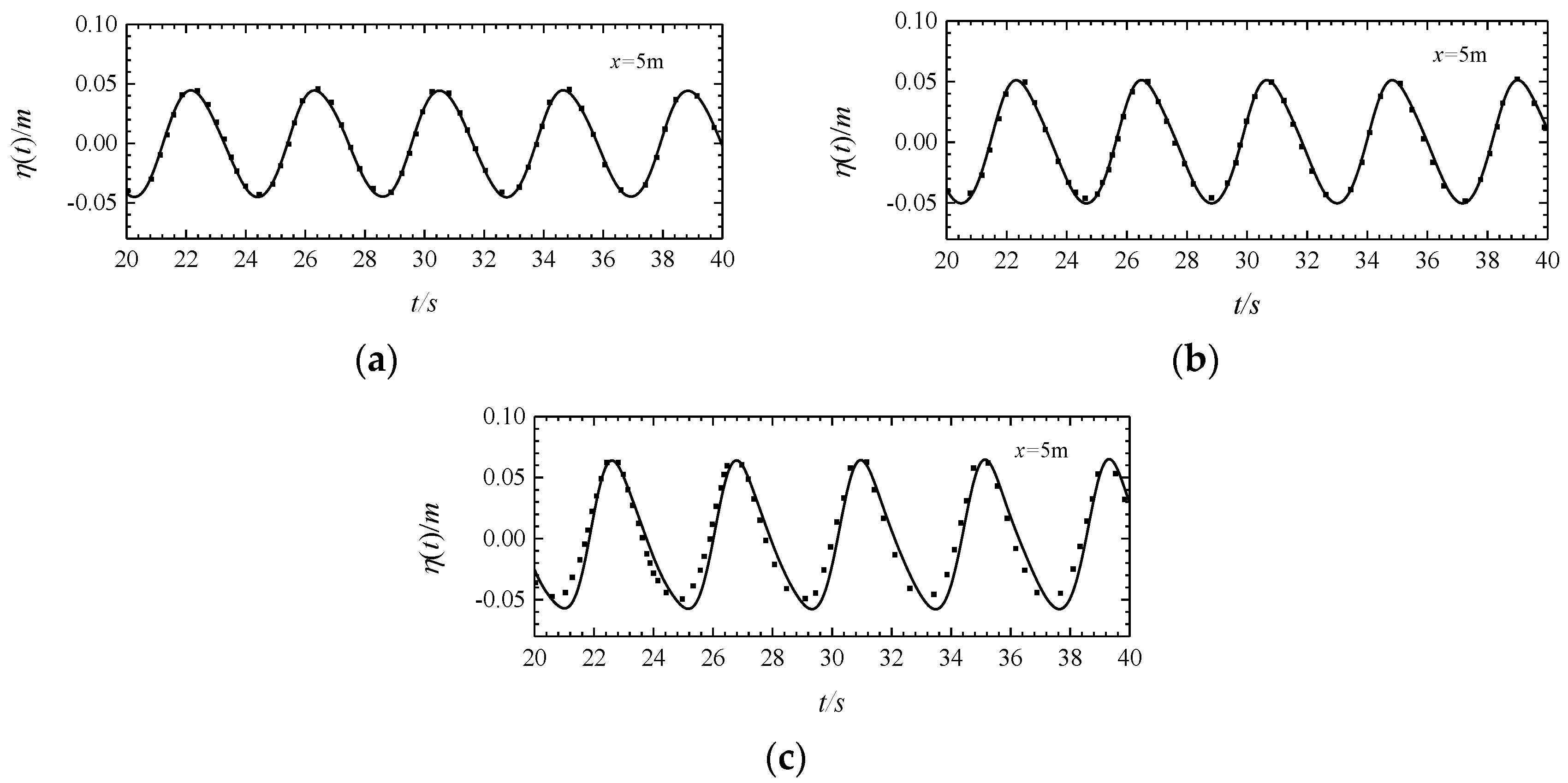
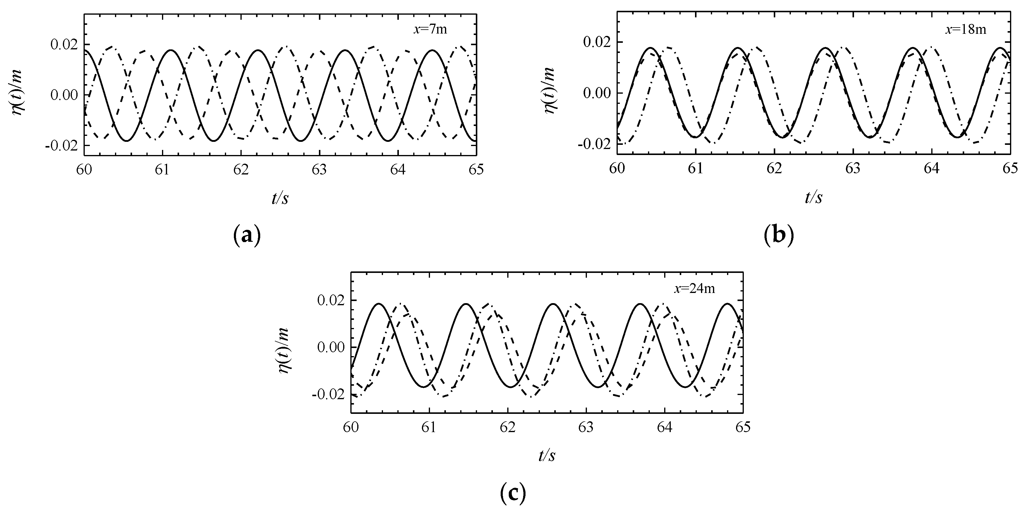
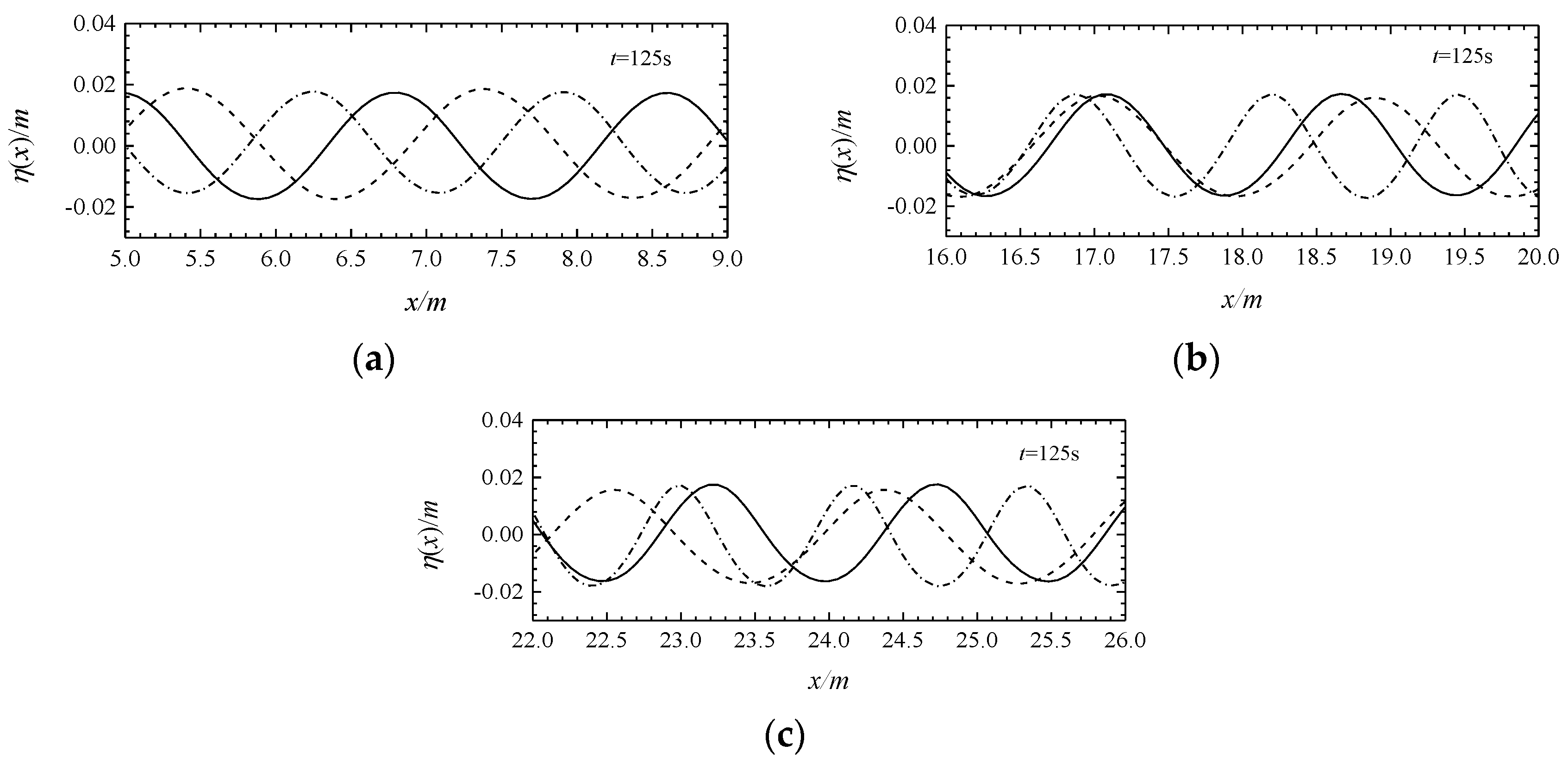
4.2.1. Numerical Simulation of Wave-Current Interactions at a Uniform Water Depth

Ning et al. [55] established a fully nonlinear numerical simulation of wave current coexistence using the time-domain, high-order, boundary-element method. They showed that the water surface satisfied the fully nonlinear free surface boundary condition. Therefore, their model can describe more accurately the nonlinear interactions between the wave and current.

The MIKE 21 BW model was used to simulate the wave-current interaction in uniform water depths. A numerical flume with a water depth of 1.0 m was set. The other parameters were as follows; the wave period was 4.17 s, the wave amplitude was 0.05 m, the wavelength was 12.55 m, the downstream flow velocity was 0.313 m/s, and the counter-current flow velocity was −0.313 m/s. The length of the flume was set to five times the wavelength. A wave-absorbing layer with a width equal to two times the wavelength was set at both ends of the flume. Space Δx = L/20 and time Δt = T/80 steps were used. The numerical simulation results of the MIKE 21 BW model were compared with those of the higher-order boundary element model.

Figure 11 shows the wave propagation simulation results in the cases along current, no-current, and counter-current conditions at x = 5 m. The numerical simulation results of the MIKE 21 BW model are consistent with the results of high-order boundary element simulation. It can be seen that Mike 21 BW model can better simulate the wave deformation under the influence of water flow. Figure 12 shows the wave propagation simulation results under the along current, no-current, and counter-current conditions at x = 10 m, respectively. Figure 11c and Figure 12c show that in the counter-current environment, the calculation results of the MIKE 21 BW model are slightly different from those of the higher-order boundary element simulations, with a maximum lag of ~9.5% wave period. Compared with the results in Figure 11c, the valley of Figure 12c is relatively flat, and there are small harmonics. It can be observed that as the distance from the wave source increases, the nonlinearity becomes stronger. The wave propagation in the countercurrent environment exhibits strong nonlinear characteristics. Although the MIKE 21 BW model exhibits weak nonlinearity characteristics, it can also describe the interactions between wave and countercurrent accurately.

Figure 13 shows that the wave deforms subject to the influence of the current. The wave amplitude decreases subject to the action of the downstream current and increases subject to the action of the counter current. The comparison of the numerical simulation results of the downstream, no-current, and countercurrent environments, shows that the wave exhibits an obvious phase deviation, which indicates that the wave speed changes subject to the action of the current. Thus, this indicates that the wavelength, respectively, increases and decreases subject to the downstream and countercurrent environments.

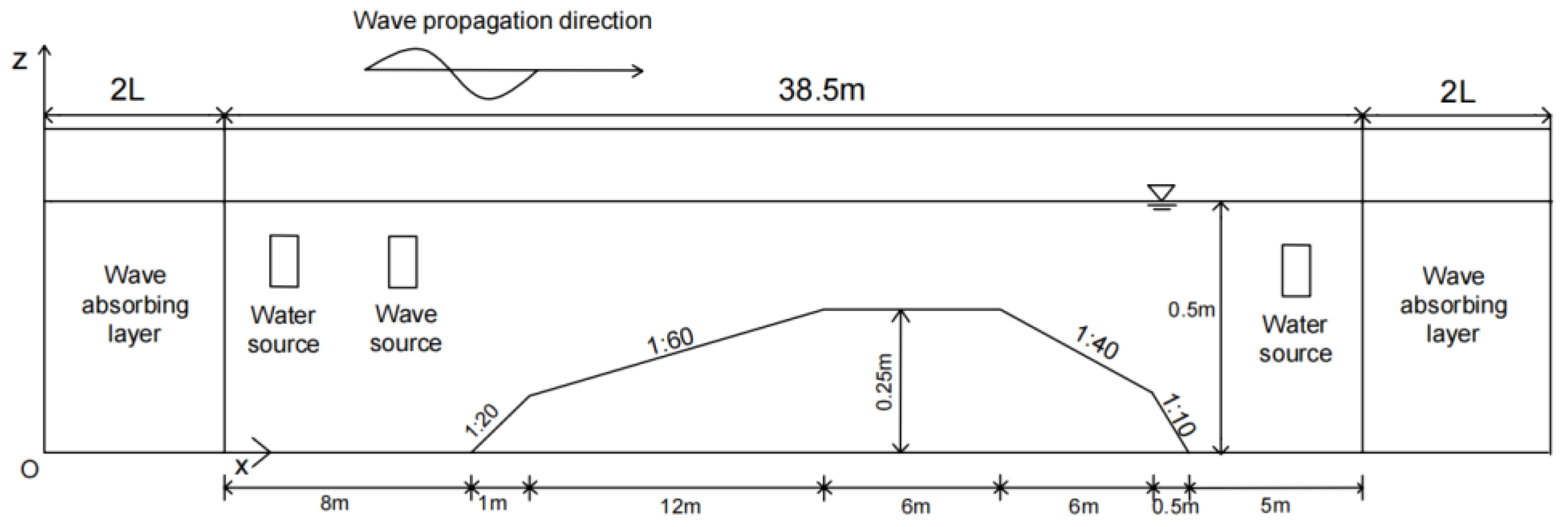
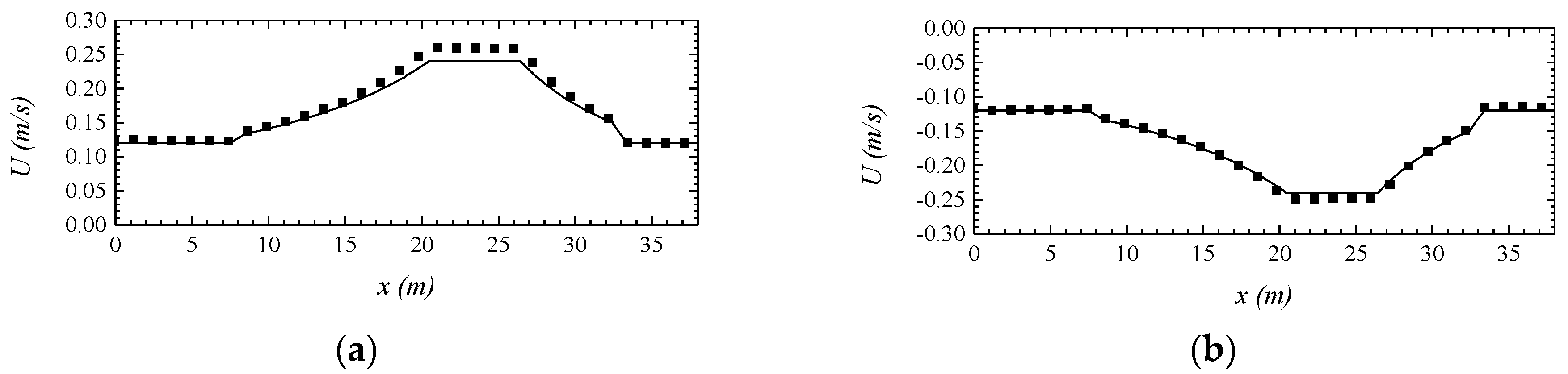
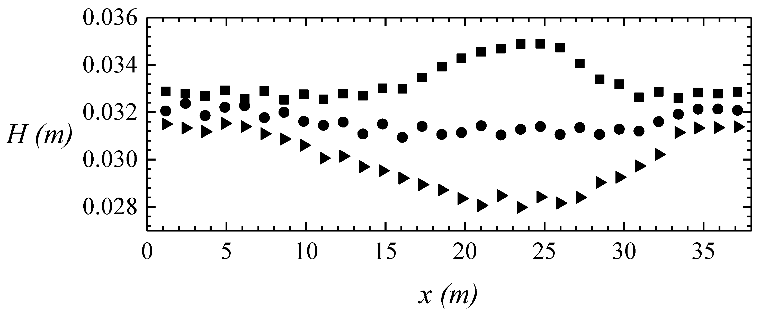
4.2.2. Numerical Simulation of Wave-Flow Interactions in Submerged Dike Topography

(1) Numerical simulation of single frequency wave interaction with water flow

The MIKE 21 BW model was used to simulate the interactions between a single-frequency wave and current in the submerged breakwater. The effects of different velocities on wave propagation were compared and analyzed. A numerical flume with a length of 38.5 m was established. The water depth in front of the submerged dike was 0.5 m, and the elevation of the top of the submerged dike was 0.25 m. The flume model is shown in Figure 14. The wave period was 1.1 s, amplitude was 0.0175 m, and the wavelength was 1.78 m. A wave-absorbing layer with a width equal to two times the wavelength was set at both ends of the water tank.

The theoretical values of the flow velocity distribution over the submerged dike topography:

$$U_c(x)=\frac{u_0{h}_0}{h(x)}$$

(24)

where μ₀ corresponds to the submerged dike before the uniform water depth flow rate; h₀ corresponds to the submerged dike before the water depth, and h(x) is the water depth change function.

For the wave numerical model of the downstream environment, the velocity of uniform water depth in front of the submerged breakwater is set at 0.12 m/s, whereas that in the wave numerical model of the counter-current environment is −0.12 m/s. It can be seen from Figure 15 that the velocity distribution calculated by MIKE 21 BW model is consistent with the theoretical value, which proves that it is feasible to simulate the water flow by setting the water flow quality source term in the model.

Figure 16 indicates that the waves have different wave heights at different flow velocities. Moreover, the wave heights change as a function of flow velocities. At the top of the submerged dike, the flow velocity and the influences of the current on the waves reach the maximum values. In the numerical model, three points (x = 7 m, 18 m, and 24 m) are used for analyses. Figure 17 shows that the wave propagates to the submerged dike and generates harmonics. The harmonic amplitude is also affected by the current. The harmonic amplitude decreases in the downstream environment and increases in the counter-current environment.

As shown in Figure 18, there are obvious phase differences among waves in different water flow conditions, which proves that the wavelength changes subject to the action of water flow. Especially when t = 125 s (Figure 19), the instantaneous wavefront diagram can visually compare the change in wavelength subject to the action of water flow. Specific values for wavelengths at different positions are listed in

Table 4. Variation of wavelength at different positions under the action of water currents.

x/m	Downstream	No-Current	Counter-Current
7	2.01	1.78	1.69
18	1.85	1.62	1.31
24	1.85	1.51	1.15

.

(2) Numerical simulation of the interaction among dual-frequency waves and water flow

Water flow also affects the generation and propagation of harmonics. Based on the numerical model of the interaction between a single-frequency wave and water flow, the simulation with double frequencies is carried out. The wave periods of the two waves are 0.9 s and 1.1 s, respectively, with a common wave amplitude of 0.0175 m.

Figure 20 shows a comparison of wave surface under the conditions of downstream, no-current, and counter-current with different flow velocities whereas Figure 21 shows the same comparison in a frequency domain diagram. The latter can intuitively compare the effect of water flow on wave harmonics.

As shown in Figure 21, in countercurrent conditions, the amplitude increase in the wave’s main frequency is marginal. However, the amplitude increase in the harmonic is larger than that of the wave without a current environment; this proves that in countercurrent conditions, the harmonic amplitude increases. When the wave is blocked by the current, the nonlinear interaction of the waves also increases.

By improving the wave source term in the mass source wave generation method to the current source term and by setting a constant current source point in the wave numerical model, the numerical simulation of waves in the current environment is realized. The MIKE 21 BW model was used to simulate the wave-current interaction between uniform water depth and submerged dike topography. The wave deformations in different directions, and for different velocities and currents were compared and analyzed. The numerical simulation results showed that the wave amplitude decreased, and the wavelength increased subject to the action of downstream flow. Subject to the action of the counter current, the amplitude increased, the wavelength decreased, and the influence of the current on the wave increased as a function of velocity. The numerical simulation results are consistent with real situations; this proves that the MIKE 21 BW model can effectively simulate wave propagation subject to the action of water flow. Furthermore, the Boussinesq equation has favorable engineering application prospects in environments with coexisting waves and currents in estuaries and bays.

5. Conclusions

In this study, the MIKE 21 BW model was used to simulate the propagation of dual-frequency waves. The theoretical solution and the Navier–Stokes equation wave model were used to verify the numerical simulation. Moreover, the Fourier transform was used to analyze and discuss dual-frequency waves. It is demonstrated that the numerical model established using the Boussinesq equation can describe more accurately the nonlinear interaction between waves. The computational efficiency of the Boussinesq equation numerical model is much higher than that of the Navier–Stokes equation wave model. Moreover, the mass source wave-making method was improved by changing the wave source term into the current source term, and a constant current source point is set in the wave numerical model to realize the numerical simulation of waves in the current environment. The numerical simulation of the wave-current interaction between uniform and variable water depths is carried out. The improved Boussinesq equation can be used to simulate the propagation of multidirectional waves from deep to shallow waters. The maximum water depth wavelength ratio reached $\mu \le 0.5$ (or $kh\approx 3.1$. Therefore, in shallow water environments, the model can describe accurately the influence of water flow on wave propagation in the coastal waters, and that has excellent engineering application prospects.

References

1. Longuet-Higgins, M.S.; Stewart, R.W. Changes in the form of short gravity waves on long waves and tidal currents. J. Fluid Mech. 1960, 8, 565–583. [Google Scholar] [CrossRef]
2. Longuet-Higgins, M.S.; Stewart, R.W. Radiation stresses in water wave; a physical discussion with application. Deep Sea Res. 1964, 4, 529–562. [Google Scholar] [CrossRef]
3. Hughes, B.A.; Stewart, R.W. Interaction between gravity waves and a shear flow. J. Fluid Mech. 1961, 10, 385–400. [Google Scholar] [CrossRef]
4. Tao, W.; Jiachun, L. Research progress of wave current interaction. Adv. Mech. 1999, 3, 331–343. [Google Scholar]
5. Jonsson, I.G. 3.2-Combinations of Waves and Currents. Dev. Geotech. Eng. 1978, 23, 162–203. [Google Scholar] [CrossRef]
6. Jonsson, I.G. Wave action flux: A physical interpretation. J. Fluid Mech. 1998, 368, 155–164. [Google Scholar] [CrossRef]
7. Brevik, I.; Bjørn, A. Flume experiment on waves and currents. I. Rippled bed. Coast. Eng. 1979, 3, 149–177. [Google Scholar] [CrossRef]
8. Brevik, I. Flume experiment on waves and currents II. Smooth bed. Coast. Eng. 1980, 4, 89–110. [Google Scholar] [CrossRef]
9. Li, Y.; Herbich, J.B. Effect of wave-current interaction on the wave parameter. In Proceedings of the 18th Conference on Coastal Engineering, Cape Town, South Africa, 14–19 November 1982. [Google Scholar] [CrossRef]
10. Swan, C.; Cummins, I.P.; James, R.L. An experimental study of two-dimensional surface water waves propagating on depth-varying currents. Part 1. Regular waves. J. Fluid Mech. 2001, 428, 273–304. [Google Scholar] [CrossRef]
11. Lian, J.J.; Zhao, Z.D. Velocity distribution of full depth water flow in wave current coexistence field. Mar. Bull. 1994, 3, 1–10. [Google Scholar]
12. Alfonsi, G.; Lauria, A.; Primavera, L. The field of flow structures generated by a wave of viscous fluid around vertical circular Cylinder Piercing the Free Surface. Process. Eng. 2015, 116, 103–110. [Google Scholar] [CrossRef] [Green Version]
13. Dong, G.; Fu, R.; Ma, Y.; Fang, K. Simulation of unidirectional propagating wave trains in deep water using a fully non-hydrostatic model. Ocean Eng. 2019, 180, 254–266. [Google Scholar] [CrossRef]
14. Ai, C.F.; Ma, Y.X.; Yuan, C.F.; Dong, G.H. Development and assessment of semi-implicit nonhydrostatic models for surface water waves. Ocean Modell. 2019, 144, 101489. [Google Scholar] [CrossRef]
15. Ruffini, G.; Briganti, R.; Alsina, J.M.; Brocchini, M.; Dodd, N.; McCall, R. Numerical modelling of flow and bed evolution of bichromatic wave groups on an intermediate beach using nonhydrostatic xbeach. J. Waterw. Port Coast. Ocean Eng. 2020, 146, 04019034. [Google Scholar] [CrossRef]
16. Thomas, G.P. Wave-current interactions: An experimental and numerical study. Part 1. Linear waves. J. Fluid Mech. 1981, 110, 457–474. [Google Scholar] [CrossRef]
17. Thomas, G.P. Wave-current interactions: An experimental and numerical study. Part 2. Nonlinear waves. J. Fluid Mech. 1990, 216, 505–536. [Google Scholar] [CrossRef]
18. Wolf, J.; Prandle, D. Some observations of wave–current interaction. Coast. Eng. 1999, 37, 471–485. [Google Scholar] [CrossRef]
19. Sørensen, O.R.; Kofoed-Hansen, H.; Jones, O.P. Numerical modeling of wave-current interaction in tidal areas using an unstructured finite volume technique. Coastal Eng. 2007, 1, 653. [Google Scholar] [CrossRef]
20. Baschek, B. Wave-current interaction in tidal fronts. In 14th ‘Aha Huliko’a Winter Workshop 2005: Rogue Waves; Muller, P., Garrett, C., Eds.; Honolulu, HI, USA, 2005; pp. 131–138. Available online: http://www.soest.hawaii.edu/PubServices/2005pdfs/Baschek.pdf (accessed on 22 November 2022).
21. Yan, Y.X. Mathematical model of wave current interaction in tidal estuary area. Ocean. Eng. 1989, 3, 47–56. [Google Scholar]
22. Li, Y.C.; Zhang, Y.G. Theoretical study of nonlinear wave current interaction using Boussinesq equation. Res. Dev. Hydrodyn. Part A 1996, 2, 205–211. [Google Scholar]
23. Chen, Q.; Madsen, P.A.; Schäffer, H.A.; Basco, D.R. Wave-current interaction based on an enhanced Boussinesq approach. Coast. Eng. 1998, 33, 11–39. [Google Scholar] [CrossRef]
24. Zou, Z.L.; Hu, P.C.; Fang, K.Z.; Liu, Z.B. Boussinesq-type equations for wave–current interaction. Wave Motion 2013, 50, 655–675. [Google Scholar] [CrossRef]
25. Wang, Y.L.; Zhang, H.S. Numerical simulation of nonlinear wave propagation in non-uniform flow. J. Mech. 2007, 6, 732–740. [Google Scholar]
26. Zhang, H.S.; Zhao, H.J.; Ding, P.X.; Miao, G.P. Wave propagation deformation in non-uniform flow waters. J. Mech. 2007, 3, 325–332. [Google Scholar]
27. Hong, G.W.; Feng, W.B.; Zhang, H.S. Numerical simulation of wave propagation in coastal and estuarine waters. J. Hohai Univ. Nat. Sci. Ed. 1999, 2, 4–12. [Google Scholar]
28. Wu, Y.S.; Lian, J.J.; Wang, Z.Y.; Zhang, Q.H. Wave current interaction model. Water Resour. 2002, 04, 13–17. [Google Scholar]
29. Liu, Y.Z.; Shi, Z. Mathematical model of wave current interaction in estuaries. Mar. Sci. 2001, 05, 42–46. [Google Scholar]
30. Teles, M.J.; Pires-Silva, A.A.; Benoit, M. Numerical modelling of wave current interactions at a local scale. Ocean Modell. 2013, 68, 72–87. [Google Scholar] [CrossRef]
31. Li, H.T.; Zhou, E.X.; Gou, J.F.; Ha, J.Q.; Liu, Y.F.; Wang, G.; Qin, L.R.; Li, H.H. Research on wave making method for numerical simulation of bichromatic wave. Water Conserv. Hydropower Technol. 2019, 50, 155–166. [Google Scholar]
32. Brorsen, M.; Larsen, J. Source generation of nonlinear gravity waves with the boundary integral equation method. Coast. Eng. 1987, 11, 93–113. [Google Scholar] [CrossRef]
33. Lin, P.; Liu, P.L.-F. Internal wave-maker for Navier–Stokes equations models. J. Waterw. Port Coastal Ocean Eng. 1999, 125, 207–215. [Google Scholar] [CrossRef]
34. Wei, G.; Kirby, J.T.; Sinha, A. Generation of waves in Boussinesq models using a source function method. Coast. Eng. 1999, 36, 271–299. [Google Scholar] [CrossRef]
35. Chen, M.Y.; Zhang, H.S.; Zhou, E.X.; Xu, D. Numerical bichromatic wave generation using designed mass source function. J. Math. 2021, 2021, 1–9. [Google Scholar] [CrossRef]
36. Ha, T.; Lin, P.; Cho, Y. Generation of 3D regular and irregular waves using Navier–Stokes equations model with an internal wave maker. Coast. Eng. 2013, 76, 55–67. [Google Scholar] [CrossRef]
37. Li, B.X.; Yu, L.X.; Zhang, N.C. Establishment and application of a numerical two-dimensional random wave flume. Mar. Bull. 2004, 5, 1–9. [Google Scholar]
38. Gao, X.P.; Zeng, G.D.; Zhang, Y. Wave creation and damped wave dissipation in irregular wave value flumes. J. Oceanogr. 2002, 2, 127–132. (In Chinese) [Google Scholar]
39. Wang, X.; Lin, Z.Y.; You, Y.X. Numerical wave generation methods for internally isolated wave mass sources in two-layer fluids. J. Shanghai Jiaotong Univ. 2014, 6, 850–855. [Google Scholar]
40. Ning, D.Z.; Teng, B.; Zhou, B.Z.; Liu, Z. Application of the source wave creation method to a three-dimensional fully non-linear numerical wave flume. J. Dalian Marit. Univ. 2008, 2, 1–5. [Google Scholar]
41. Gobbi, M.F.; Kirby, J.T. Wave evolution over submerged sills: Tests of a high-order Boussinesq model. Coast. Eng. 1999, 37, 57–96. [Google Scholar] [CrossRef]
42. Andrzej, M. Energy conserving numerical solutions of simplified turbulence equations. Math. Tech. Report. 1990, 1175–1180. [Google Scholar] [CrossRef]
43. Mohapatra, S.C.; Fonseca, R.B.; Guedes Soares, C. Comparison of analytical and numerical simulations of long no linear internal solitary waves in shallow water. J. Coastal. Res. 2018, 34, 928–938. [Google Scholar] [CrossRef]
44. Mohapatra, S.C.; Gadelho, J.F.M.; Guedes Soares, C. Effect of interfacial tension on internal waves based on Bousinesq equations in two-layer fluids. J. Coastal. Res. 2019, 35, 445–462. [Google Scholar] [CrossRef]
45. Dinvay, E. Well-posedness for a Whitham–Boussinesq system with surface tension. Math. Phys. Anal. Geom. 2020, 23, 1–27. [Google Scholar] [CrossRef]
46. Karaagac, B.; Ucar, Y.; Esen, A. Dynamics of modified improved Boussinesq equation via Galerkin finite element method. Math. Meth. Appl. Sci. 2020, 43, 1–17. [Google Scholar] [CrossRef]
47. Yao, S.W.; Islam, M.E.; Akbar, M.A.; Inc, M.; Adel, M.; Osman, M.S. Analysis of parametric effects in the wave profile of the variant Boussinesq equation through two analytical approaches. Open Phys. 2022, 20, 778–794. [Google Scholar] [CrossRef]
48. Fang, K.Z.; Liu, Z.B.; Wang, P.; Wu, H.; Sun, J.W.; Yin, J. Modeling solitary wave propagation and transformation over complex bathymetries using a two-layer Boussinesq model. Ocean. Eng. 2022, 265, 112549. [Google Scholar] [CrossRef]
49. Madsen, P.A.; Sørensen, O.R. A new form of the Boussinesq equations with improved linear dispersion characteristics. Part 2. A slowly-varying bathymetry. Coast. Eng. 1992, 18, 183–204. [Google Scholar] [CrossRef]
50. Madsen, P.A.; Murray, R.; Sørensen, O.R. A new form of the Boussinesq equations with improved linear dispersion characteristics. Coast. Eng. 1991, 15, 371–388. [Google Scholar] [CrossRef]
51. Madsen, P.A.; Sørensen, O.R.; Schäffer, H.A. Surf zone dynamics simulated by a Boussinesq type model. Part I: Model description and cross-shore motion of regular waves. Coast. Eng. 1997, 32, 255–288. [Google Scholar] [CrossRef]
52. Madsen, P.A.; Sørensen, O.R.; Schäffer, H.A. Surf zone dynamics simulated by a Boussinesq type model. Part II: Surf beat and swash zone oscillations for wave groups and irregular waves. Coast. Eng. 1997, 32, 289–320. [Google Scholar] [CrossRef]
53. Sørensen, O.R.; Schäffer, H.A.; Madsen, P.A. Surf zone dynamics simulated by a Boussinesq type model. Part III: Wave-induced horizontal nearshore circulations. Coast. Eng. 1998, 33, 155–176. [Google Scholar] [CrossRef]
54. Sørensen, O.R.; Schäffer, H.A.; Sørensen, L.S. Boussinesq-type modelling using an unstructured finite element technique. Coast. Eng. 2004, 50, 181–198. [Google Scholar] [CrossRef]
55. Ning, D.Z.; Chen, L.F.; Tian, H.G. Fully non-linear numerical flume model for wave-flow mixing action. J. Harbin Eng. Univ. 2010, 11, 1450–1455. [Google Scholar]
Figure 1. Schematic diagram of the MIKE 21 BW 2D model discrete method.
Jmse 11 00299 g001
Figure 2. Schematic diagram of the numerical model for the mass source wave-generating method.
Jmse 11 00299 g002
Figure 3. Comparison of the wavefront at x = 1L2 (a), x = 2L2 (b), x = 6L2 (c), x = 10L2 (d) of the MIKE 21 BW model (solid line) and the theoretical solution (dashed line) (operating condition C1).
Jmse 11 00299 g003
Figure 4. Frequency domain plots of wave simulation results at x = 1L2 (a), x = 2L2 (b), x = 6L2 (c), x = 10L2 (d) of the MIKE 21 BW model (○) and the theoretical solution (┼) (operating condition C1).
Jmse 11 00299 g004aJmse 11 00299 g004b
Figure 5. Comparison of the wavefront at x = 1L2 (a), x = 2L2 (b), x = 6L2 (c), x = 10L2 (d) of the MIKE 21 BW model (solid line) and the theoretical solution (dashed line) (operating condition C2).
Jmse 11 00299 g005aJmse 11 00299 g005b
Figure 6. Frequency domain plots of wave simulation results at x = 1L2 (a), x = 2L2 (b), x = 6L2 (c), x = 10L2 (d) of the MIKE 21 BW model (○) and the theoretical solution (┼) (operating condition C2).
Jmse 11 00299 g006
Figure 7. Comparison of wavefronts at x = 1L2 (a), x = 2L2 (b), x = 6L2 (c), x = 10L2 (d) in the MIKE 21 BW model (solid line) and the Navier–Stokes model (dashed line) (operating condition C1).
Jmse 11 00299 g007
Figure 8. Frequency domain plots of wave simulation results at x = 1L2 (a), x = 2L2 (b), x = 6L2 (c), x = 10L2 (d) for the MIKE 21 BW model (○) and the Navier–Stokes model (╳) (operating condition C1).
Jmse 11 00299 g008
Figure 9. Comparison of wavefronts at x = 1L2 (a), x = 2L2 (b), x = 6L2 (c), x = 10L2 (d) in the MIKE 21 BW model (solid line) and the Navier–Stokes model (dashed line) (operating condition C2).
Jmse 11 00299 g009
Figure 10. Frequency domain plots of wave simulation results at x = 1L2 (a), x = 2L2 (b), x = 6L2 (c), x = 10L2 (d) for the MIKE 21 BW model (○) and the Navier–Stokes model (╳) (operating condition C2).
Jmse 11 00299 g010
Figure 11. Wavefront ratio (at x = 5 m) of the MIKE 21 BW model (solid line) to the boundary element model (■) in downstream (a), no-current (b), counter current (c) environment.
Jmse 11 00299 g011
Figure 12. Wavefront ratio (at x = 10 m) of the MIKE 21 BW model (solid line) to the boundary element model (■) in downstream (a), no-current (b), counter-current (c) environment.
Jmse 11 00299 g012
Figure 13. Wavefront ratios at x = 5 m (a) and x = 10 m (b) for different flow conditions in the MIKE 21 BW model (solid line for no-current, dashed line for downstream, dotted line for counter-current).
Jmse 11 00299 g013
Figure 14. Schematic diagram of the submerged dike topographic wave flow interaction model.
Jmse 11 00299 g014
Figure 15. Velocity distribution of MIKE 21 BW model (■) and theoretical value (solid line) in submerged dike topography: (a) downstream, (b) counter current.
Jmse 11 00299 g015
Figure 16. Distribution of environmental wave heights along the downstream (▼), no-current (●), and counter-current (■) of MIKE 21 BW model.
Jmse 11 00299 g016
Figure 17. Frequency domain plots of wave simulation results at three points x = 7 m (a), 18 m (b), and 24 m (c) of MIKE 21 BW model. in downstream (╳), no-current (○), and counter-current (△).
Jmse 11 00299 g017
Figure 18. Comparison of wave surfaces at three points x = 7 m (a), 18 m (b), and 24 m (c) of downstream (dotted line), no-current (solid line), and counter-current (dotted line) of MIKE 21 BW model.
Jmse 11 00299 g018
Figure 19. MIKE 21 BW model downstream (dotted line), no-current (solid line), and counter-current (dotted line) simulated instantaneous wavefront in different positions such as (ac).
Jmse 11 00299 g019
Figure 20. Comparison of wave surfaces at three points x = 7 m (a), 18 m (b), and 24 m (c) of MIKE 21 BW model with dual-frequency waves in downstream (dotted line), no-current (solid line), and counter-current (dotted line).
Jmse 11 00299 g020
Figure 21. Frequency domain plots of wave simulation results at three points x = 7 m (a), 18 m (b), and 24 m (c) of MIKE 21 BW model with dual-frequency wave in downstream (╳) no-current (○) and counter-current (Δ).
Jmse 11 00299 g021