
Reconstruction Methods in Oceanographic Satellite Data Observation—A Survey

1
Environmental Data Analysis Laboratory, Faculty of Science, University of Split, 21000 Split, Croatia
2
University Department of Marine Studies, University of Split, 21000 Split, Croatia
*
Author to whom correspondence should be addressed.
J. Mar. Sci. Eng. 2023, 11(2), 340; https://doi.org/10.3390/jmse11020340
Submission received: 28 December 2022
/
Revised: 14 January 2023
/
Accepted: 30 January 2023
/
Published: 3 February 2023
(This article belongs to the Special Issue Recent Scientific Developments in Ocean Observation)
Abstract
:Oceanographic parameters, such as sea surface temperature, surface chlorophyll-a concentration, sea surface ice concentration, sea surface height, etc., are listed as Essential Climate Variables. Therefore, there is a crucial need for persistent and accurate measurements on a global scale. While in situ methods tend to be accurate and continuous, these qualities are difficult to scale spatially, leaving a significant portion of Earth’s oceans and seas unmonitored. To tackle this, various remote sensing techniques have been developed. One of the more prominent ways to measure the aforementioned parameters is via satellite spacecraft-mounted remote sensors. This way, spatial coverage is considerably increased while retaining significant accuracy and resolution. Unfortunately, due to the nature of electromagnetic signals, the atmosphere itself and its content (such as clouds, rain, etc.) frequently obstruct the signals, preventing the satellite-mounted sensors from measuring, resulting in gaps—missing data—in satellite recordings. One way to deal with these gaps is via various reconstruction methods developed through the past two decades. However, there seems to be a lack of review papers on reconstruction methods for satellite-derived oceanographic variables. To rectify the lack, this paper surveyed more than 130 articles dealing with the issue of data reconstruction. Articles were chosen according to two criteria: (a) the article has to feature satellite-derived oceanographic data (b) gaps in satellite data have to be reconstructed. As an additional result of the survey, a novel categorising system based on the type of input data and the usage of time series in reconstruction efforts is proposed.
1. Introduction
Oceanographic variables represent a significant subsection of Essential Climate Variables (ECV) [1,2,3]. Similar to all other ECVs, if oceanographic variables are to be used for analysis and forecasting purposes, persistent measuring and monitoring is required, both locally and globally. Generally, measuring methods can be divided into two distinct categories: in situ methods and remote sensing methods [4]. Depending on the specific measurement needs, one or the other method provides a better fit. For example, in situ methods, despite being difficult to perform accurately, are vastly superior compared to remote sensing methods when dealing with localised measurements, allowing for maximum accuracy and significantly higher spatial and temporal resolution [4]. However, scaling the in situ measurement coverage both spatially and temporally, in most cases, is exponentially difficult in regard to financial costs and logistical planning. This issue becomes even more prominent when one’s aim is to achieve global coverage. This issue can be rectified by implementing remote sensing methods. Remote sensing encompasses measuring techniques based on analysing the electromagnetic signal retrieved from a target location [5]. Remote sensors are particularly useful when mounted on satellites [4,6], allowing for vast spatial coverage with relatively high temporal resolution.
As mentioned, the crux of remote sensing is the analysis of the detected electromagnetic signal. Depending on the target variable, a certain range of the electromagnetic spectrum is considered [4,6]. Furthermore, depending on the mentioned range, the measurement is carried out either actively or passively. Active measurement implies emission of the signal and detection of the subsequent reflected signal. Examples of active measurement include sea surface height and sea roughness. When measuring the two, a signal from the microwave range of the spectrum is emitted. The travel time and strength of the backscattered are measured and used as a starting point for the derivation of the aforementioned variables [4,6].
Not all oceanographic variables can be detected using the active measurement. Some of them rely on passive measurements: meaning the detection of naturally emitted and/or reflected signals (sunlight) from the sea. This infers that different parts of the electromagnetic spectrum are considered: visible light for ocean colour (and subsequently the concentration of chlorophyll-a suspended particulate matter, organic and inorganic carbon, coloured dissolved matter, etc.) [7,8] and infrared for sea surface temperature [9,10]. This, however, poses a problem, especially when considering satellite-based remote sensing because not all parts of the electromagnetic spectrum contain the same penetrative properties [11]. While the Earth’s atmosphere is generally transparent for some wavelengths (such as microwaves), other parts of the spectrum can be significantly attenuated [11]. Due to non-penetrative nature of visible and infrared light cloud cover significantly diminished the area from which signals can be retrieved [12,13,14,15]. Other factors, such as unfavourable sun glint and high aerosol loading [16,17,18], further diminish spatial coverage. Even successful measurements are subject to removal in efforts of quality control [19,20,21,22,23]. All these negative influences result in gaps in satellite data, which hinders its usefulness.
Reducing the occurrences of gaps in satellite data are the next natural step. While improvements to the sensors [24,25] might reduce these gaps in future measurements, it will not help remove the gaps in already obtained data. Therefore, in the past two decades, significant efforts have been poured into various data-driven reconstruction techniques. By analysing existing available data, these techniques aim to infer the values of missing data in an effort to create complete, gap-free datasets. This paper provides a review of these methods when applied to oceanographic data. Among the data, sea surface temperature (SST) and surface chlorophyll-a concentration () are significantly more prominent than the rest. Because some reconstruction approaches may simultaneously utilise data at various processing stages, next, Section 2 introduces the handling and derivation of satellite data, from raw data to final product. Section 3 briefly summarises the most popular gap-filling techniques used in satellite oceanography. Finally, Section 4 showcases examples of those techniques being applied in literature throughout the years.
2. Satellite Data
This section will briefly guide the reader through the nuances of what satellite data actually represents, how it is gathered and processed—from raw electromagnetic signals to mapped geophysical variables. In order not to digress too far from the main idea of the paper, only and SST products will be explored and explained.
2.1. Levels of Data
Obtaining measurements via satellites is an expensive and complex process—from the initial measurements, through signal conversion to the final data acquisition. While the exact nuances of this process may differ from one organisation to the other [26,27], the backbone procedure is mostly the same. Specifically, this subsection will shed light on the process implemented by NASA [26]. Depending on the process steps applied to the satellite data, the data are separated into specific stages called levels.
The first stage, level 0, refers to the initial content and format of data retrieved from the satellite after downloading the files to data cloud; this includes anything and everything that the satellite generates. These data have not been altered in any way, shape or form. At this level, data are not usable for any scientific purposes, but the data are always saved as it can be used for recreating any subsequent data level in case of data loss. Additionally, the data are stored in specific packets, referred to as the Consultative Committee for Space Data Systems (CCSDS) packets [28].
Level 1 is usually subdivided into two sub-levels. Level 1A combines the CCSDS packets and restructures the data in units reflecting the way the sensor measures: for example, if the sensor in question is a scanner, then the unit of storage/structure is the set of pixels detected during that scan. Apart from measurement data, satellite navigation and other telemetry data are acquired. The final step of level 1A separates data into timed chunks (e.g., 5-min chunks), as a means of data size management [28]. Level 1B calibrates and geolocates level 1A data. Level 1A data comes in the form of integer counts. Calibration converts these counts into physical units, such as radiance/reflectance and brightness temperature. During calibration, instrument corrections are applied—nonlinear signal responses, temperature effects, sensor degradation and other instrument effects are all taken into account when considering instrument correction [4]. After the correction has been applied, navigation data of the spacecraft are combined with the geometry model of the instrument to determine the origin location of each measurement. This way, the data are geolocated [28]. Generally speaking, level 1 data are not an overly popular target for gap-filling [29,30,31,32].
Up to this point, satellite data can be viewed as “engineering data”—information on the spacecraft position and viewing angle, effects of instrument imperfections on data and so on. Level 2 data are the first instance of data being formatted into “scientific data”. Level 2 data are the output of various algorithms, some of which will be explored in Section 2.2 and Section 2.3, which take level 1B data as input. These algorithms may require ancillary data—data regarding different parameters, such as atmospheric water vapour, surface pressure, ozone layer thickness, etc., which are retrieved from sources outside the satellite in question itself. Level 2 data also contain quality flags—various parameters put in place to ensure data are within uncertainty standards set by the scientific community [28]. In the context of gap-filling, level 2 data are utilised for local/regional instances [33,34,35,36,37,38,39,40,41,42,43,44,45,46,47,48,49,50,51,52,53,54,55,56,57].
After level 2 data have been obtained, all instances of it from a single day can be combined spatially to create composites, creating level 3 data. While these composites usually contain a day’s worth of information, composition can be carried out along the time axis, combining progressively longer time periods (8 days, month, season, year and finally entire duration of the satellite mission) [28]. Naturally, since level 3 data do not have spatial constrains, unlike level 2 data, it should be obvious that it is the most popular choice when dealing with data reconstruction [58,59,60,61,62,63,64,65,66,67,68,69,70,71,72,73,74,75,76,77,78,79,80,81,82,83,84,85,86,87,88,89,90,91,92,93,94,95,96,97,98,99,100,101,102,103,104,105,106,107,108,109,110,111,112,113,114,115,116,117,118,119,120,121,122,123,124,125,126,127,128,129,130,131,132,133,134,135,136,137,138,139,140,141,142,143,144,145,146,147,148,149,150,151,152,153,154,155,156,157,158].
The final step in data processing is the optional level 4. Level 4 data are optional in a sense that level 3 data are already well-suited and are used as-is by the scientific community. This level represents either a new variable type of data that has been derived from previously obtained satellite data (e.g., ocean primary productivity data are derived from data [26]) or satellite data that have been augmented in some way [26]. This augmentation can be achieved via an increase in spatial resolution [155,159,160,161], or, more popularly as will be showcased in Section 4, via missing data reconstruction. Some of the reviewed articles utilised level 4 data for gap-filling proof-of-concept purposes [162,163,164].
2.2. Surface Chlorophyll—A Concentration
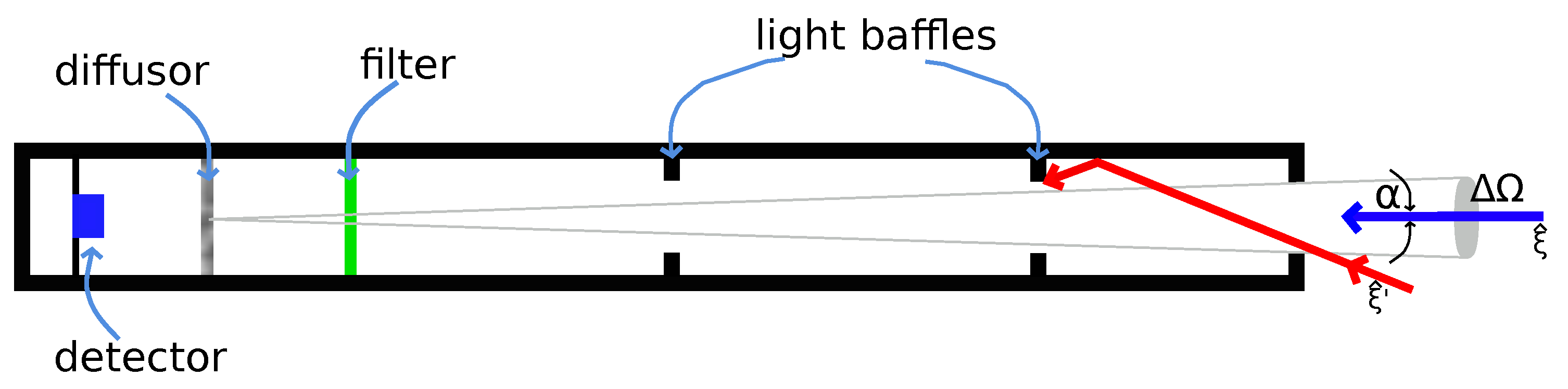
Radiance and reflectance were mentioned in previous the subsection. In order to better grasp the physical characteristics of these variables, they are best explained through the design behind their respective sensors. is derived from ocean colour—visible light being reflected from the sea towards the satellite. Measuring the intensity of this light can be carried out via a Gershun tube radiometer [165]. The design of the radiometer is displayed in Figure 1. On one end of the tube is a hole of a fixed size which allows light to enter the device. Entering the hole, the light passes through the collection tube, which has internal light baffles. By building the hole and the collection tube to be of specific proportions, along with the baffles, incoming light is filtered according to the incoming angle, denoted . This angle is usually to . If any light enters from an angle greater than , the light is blocked and does not affect the measurement. Knowing , the viewing solid angle of the detector is given by [165]. Passing through the collection tube, light is filtered according to wavelength . This filter allows for a certain bandwidth to pass through. In most cases today, the bandwidth is around 10 nm, while hyperspectral instruments may shrink this to just a few nanometers [24,25,165]. Before hitting the photo-sensitive detector located at the end of the tube, light is diffused over an area . Knowing the properties of the light that is landing on the detector, radiance L is defined as [165]:
Essentially radiance is the power of the light radiation at a specific wavelength per unit solid angle per unit area. Remove the collection tube dependence on the viewing angle and, instead of radiance, irradiance E is measured [165]:
Depending onthe orientation of the device, the irradiance measured is usually either downwelling or upwelling [165].
Figure 1.
Cross-section of the Gershun tube radiometer.

Unfortunately, property of both radiance and irradiance is sensitive to receiving radiation due to sea surface perturbations and, as such, they usually are not implemented individually. However, since they exhibit a certain degree of correlation, their ratio attenuates this sensitivity enough to be usable for scientific purposes [165]. This ratio can be defined in multiple ways [165], but the most used one in ocean colour sciences is the so-called remote-sensing reflectance [165]:
where the subscript denotes evaluation just above the sea surface, and subscript denotes water-leaving (or upwelling) radiance. Angles and denote the upward direction of the light exiting the water [165]. Combining this information with the level division provided in the previous subsection, it is prudent to note how raw radiance and raw irradiance are practically the only level 1 data available. Every variable derived henceforth, including water-leaving radiance and normalised water-leaving radiance , is considered to be at least level 2 data as some algorithms (e.g., the atmospheric correction) need be applied [26,165].
With radiances and reflectances explained, algorithms become much more comprehensible. Depending on the data provider, a variety of algorithms may be used, on both global and regional scales [156,166,167,168,169,170,171,172,173,174]. Most of these algorithms follow one of the two general formula shapes, depending on if they estimate in oligotrophic [168] or eutrophic [166] waters. For example, NASA [26] offers a global weighted blend of both algorithms. The oligotrophic algorithm [168] is given as:
where is the so-called colour-index, and , and are the sensor appropriate wavelengths. is then used to estimate :
For higher concentrations, the eutrophic (or the standard) algorithm is used [166]:
Here, denotes the maximum value of between several different wavelengths [166]. Exact values of depend on the scale and region where the algorithm is applied [166,170,171,172,174].
has been targeted for gap-filling via various methods since the early 2000s [84,131,137], but the popularity soared in the past several years [30,31,33,34,35,36,37,38,39,40,41,42,43,44,45,46,50,51,52,53,57,58,59,60,61,62,63,64,65,66,67,68,69,70,71,72,73,74,75,76,77,78,79,80,81,82,83,85,86,87,88,89,90,91,92,93,132,133,134,135,136,138,148,155,156,157].
2.3. Sea Surface Temperature
Measurement devices developed for SST measurements are similar in design to the ones developed for [4,6,175]. The only difference between the two is, whereas the first measures visible light and derives radiance (and related variables), SST measuring devices measure other parts of the electromagnetic spectrum and derive brightness temperature . Measuring SST using remote sensing methods is based on Planck’s law: every body emits a flux of energy, , proportional to the body’s temperature, T, at a given wavelength . The flux is given by:
where h is the Planck’s constant, c is the speed of light, and k is Boltzmann’s constant. Naturally, the spectrum of the flux is continuous regarding ; however, this does not mean that measuring of sea’s temperature can be achieved at any given wavelength. Generally, three conditions are considered when determining the target wavelength(s). Firstly, the sea should emit a detectable amount of energy given the usual temperature. Next, since the sensors are mounted on satellite flying above the atmosphere, the signal reaching the sensor should be as unaffected by the atmosphere as possible. Finally, measuring the flux at the given wavelength should be technologically possible, not to mention practical [4,175]. All things considered, SST can be measured in the infrared and microwave part of the spectrum [4,175,176]. Both wavelength choices have their advantages and disadvantages: while infrared measurements are more accurate and achieve higher resolution, microwave measurements are more robust in terms of measuring through cloud cover [177,178]. Generally, infrared measurements are more prominent [179,180,181,182,183,184,185,186]. However, the entire infrared spectrum not is used for SST measurement. Typically, infrared sensors are designed to measure between 3–5 and 8–12 [4,187]. These spectra are usually called channels [4]. Assuming sensors are well-calibrated, the next step in SST retrieval is removal of effects of the atmosphere and its contents have on the signal. Simplified, an assumption can be made that the difference between the energy fluxes detected between two wavelengths is related to the temperatures difference between them [4,175,187]:
where subscripts i and j refer to the sensor channels. Considering that the atmospheric effects are small in these particular channels, SST can be estimated by a simple linear function [4,180,182,184,185,187,188]:
where are coefficients derived by regression analysis or in situ comparisons [4,189]. Expanding upon this linear estimation, higher accuracy can be achieved if sensor viewing angle is considered [4,183,184,186,187]:
where are the new coefficients, is the basic linear estimation of SST, and is the sensor zenith angle. Further improvements of the algorithms are mostly derived from the presented ideas. Depending on the specific sensors and product suite, different algorithms may be utilised. For example, NASA’s ocean colour suite [190] offers a variety of SST products obtained by different algorithms [183,186].
In comparison to , SST received slightly less reconstruction attention [43,44,46,47,48,49,52,54,55,56,87,88,89,90,91,94,105,106,107,108,109,110,111,112,113,114,115,116,117,118,119,120,121,122,123,124,125,126,127,128,140,141,142,143,144,145,146,147,150,151,152,153,154,162,191,192,193,194]. However, examining the timeline of the development of reconstruction methods, one can notice that, in some cases, SST is the first variable to be targeted with novel methods, sort of as a proof-of-concept. This should not necessarily be surprising, as SST is slightly more trivial to derive than , is significantly less volatile than , and microwave SST is significantly more impervious to atmospherically-induced gaps.
2.4. Other Satellite Derived Oceanographic Variables
While and SST are the most popular oceanographic variables, other types of variables are also available and have also been targeted for reconstruction. These include, but are not limited to: sea surface height/sea level anomaly (SSH/SLA) [100,101,102,103,104,139,158] sea surface salinity (SSS) [29,33,54], total suspended matter/suspended particulate matter concentration (TSM/SPM) [45,52,130,148,195], photosynthetically active radiation (PAR) [86,87], diffuse attenuation coefficient () [30,40,148,149], phytoplankton and particulate concentration (, ) [53,83,136] and so on [31,32,41,42,96,99,129,163,164].
3. Reconstruction Methods
Before delving into the details of various reconstruction methods, it is prudent to define several categories of reconstruction approaches to better make sense of similarities and dissimilarities between the approaches. Our findings show that it is possible and practical to separate the methods (and the subsequent application of the respective methods in literature) regarding two criteria: type of data used and time-instances of data used. Type of data used refers to whether or not reconstruction of target data has been achieved using additional, relevant, non-target type of data. The additional, non-target type data are referred to as proxy data. Proxy data may improve reconstruction accuracy if there is significant correlation between the target and proxy data. Mathematically, let x be the target data. Then, in a single time-instance of satellite data (a single satellite image), let represent areas of the image containing available data and areas of the image with missing data, so that:
represents the entire area of the image, where ⊕ denotes the operation of spatial composition. Let f be some reconstruction function that, for a given input, outputs the value of the target data in missing areas. Finally, let y be a proxy data. Then, two approaches may be defined:
and
or
where ∨ denotes the logic operation “or”. Equation (12) represents the non-proxy approach, while both Equations (13) and (14) represent the proxy approach. These approaches may also be called the univariate and multivariate approaches. An example of this distinction between the two is illustrated in Figure 2. For clarity, these examples are limited to one proxy data, but no such limit need exist in reality.
Similarly, data can be reconstructed with or without drawing resources from time series. Let denote the targeted image time-instance. The single time-instance approach is virtually identical to the univariate approach from Equation (12):
However, the approach with multiple time-instances is then given by:
where and denote the number of considered time-instances prior and after the targeted time-instance. In practical terms, since most satellite data have a temporal resolution of a single day, time-instances usually refer to day; if is 15 July 2014, then denotes 14 July 2014, denotes 16 July 2014 and so forth. Distinction between the two latter approaches is depicted in Figure 3. If the reconstruction is completed using information from a time series, the reconstruction is simply referred to as multitemporal, but if it draws resources from only one time-instance, it is referred to as unitemporal.
It is important to note how the two criteria are not mutually exclusive: a method may be categorised as any one of the four possible combinations: e.g., simple spatial interpolation of a single swath would be placed in the Univariate/Unitemporal category, while spatio-temporal interpolation of combined and SST data would be played in the Multivariate/Multitemporal category. It is also important to point out that these categories are not always rigid. As will be seen in the following subsections, one method might be originally developed for univariate reconstruction and subsequently minimally modified to allow for multivariate reconstruction. Therefore, rather than putting emphasis on sorting the methods themselves into these categories, it is more sensible to focus on sorting the actual reconstruction approaches, meaning the combination of method and input data. To put this categorisation system in place, Table 1 has been added.
The remainder of this section briefly presents the main idea behind the most popular reconstruction methods presented in literature. Naturally, explaining every detail and modification of every existing variation would detract too much from the main idea of this paper. Thus, should the reader wish to inquire more about a particular reconstruction method, they should refer directly to source material.
3.1. EOF/DINEOF
Empirical orthogonal functions (EOF) have been hypothesised to be useful in data interpolation [151]. EOF are calculated using singular value decomposition (SVD) [196]. A matrix X containing observations so that represents the value of the field at location at the moment , i.e.:
can be written as a succession of n column vectors size of m at moment :
This matrix may represent a set of satellite images, among other types of data [151]. Then, applying SVD, the u and v eigenvectors (sizes of m and n) are obtained:
where is the singular value, and is the adjoint of X. The decomposition is equivalent to:
By decomposing this way, u and v can be thought of as the eigenvectors of time-averaged covariance matrix and the spatially-averaged covariance matrix [151]. Since the eigenvectors are normalised, initial matrix X can be decomposed into:
where U and V are the matrices composed of columns of and , and D is the diagonal matrix so that , where is the Kronecker symbol. SVD allows for accurate approximation of X by using just the first k dominant eigenvectors instead of the complete set of q eigenvectors [197]. SVD is only applicable on complete matrices—datasets that have no missing values. This, as stated before, is not a given in the domain of satellite oceanography. Since EOF aims to describe the signal, combinations of dominant EOF might be used to estimate missing values [151]. In order to apply EOF for this purpose, a certain setup is needed. Firstly, let I denote the set of missing data, containing missing data. is the reconstructed dataset, is the observed dataset with missing data, and is the dataset with missing data filled in. is obtained by setting the missing values of I to 0. After that, SVD is applied to , so that [151]:
Then, using the first N dominant eigenvectors, interpolated values of can be obtained [151]:
and consist of N first spatial and temporal EOF. Now, can be written as:
where is zero for all non-missing data points. This procedure can be repeated again:
where denotes filled data that have been subjected to mentioned estimation twice. Theoretically, this procedure can be repeated indefinitely. In practice, this procedure goes on until convergence of estimation error based on a cross-validation technique [193]. This method is more popularly known as Data INterpolating Empirical Orthogonal Functions (DINEOF) [193].
DINEOF, its variations and other EOF-based reconstruction methods are arguably the most popular reconstruction methods: its development sparked a boom in data reconstruction, and it has served in many instances as benchmark for reconstruction accuracy comparison [29,30,31,33,34,37,39,40,43,44,45,50,51,52,55,58,59,63,66,69,70,71,72,73,74,77,78,79,81,82,85,87,88,89,90,91,92,93,95,101,102,104,105,107,119,120,125,127,128,130,133,135,142,143,144,148,150,151,157,162,191,193,194,195].
3.2. Support Vector Regression
One of the older methods utilised for dealing with regression problems is Support Vector Regression (SVR) [198]. Support Vectors, as the name suggest, represent data points which serve as a basis for decisions implemented for the rest of the data: from classification to regression, etc. [198,199]. To explain this approach, let be a set of independent variables obtained during N measurements and let be a set of corresponding dependent (or target) variables. SVR then primarily aims to determine the function f which combines them. For a linear problem, this function is expressed as:
so that the error margin between the actual measurements and estimations is . Explicitly, let f be:
so that a, x and b represent vectors, and ⊙ represents scalar product. The secondary aim of SVR is to minimise the slope a. This can be achieved through minimising the norm , so that the optimal hyperplane between the data can be achieved [200]. With these two conditions in place, SVR is essentially an optimisation problem:
- s. t.;
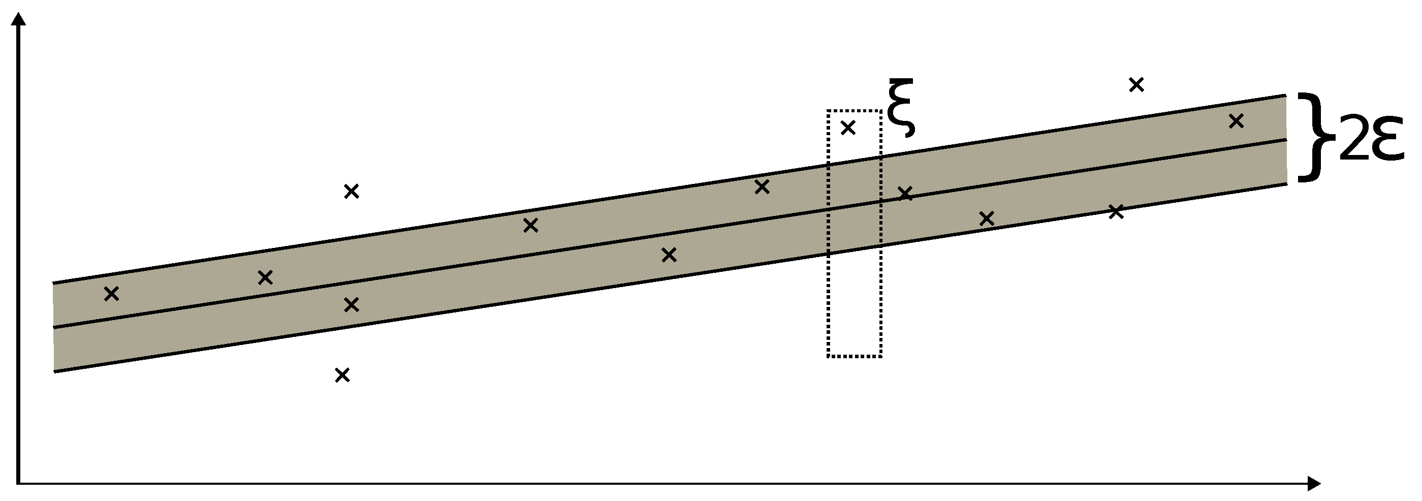
The formulation assumes both conditions can be fulfilled simultaneously, which may or may not be possible for a given problem [198]. To rectify this, slack variables and are introduced, practically making the error margin flexible [201]. Visualisation of and is presented in Figure 4. Optimisation problem now becomes:
- s. t.;
- and
- .
This is the backbone of SVR [201]. SVR can be applied to nonlinear problems; delinearisation is achieved via Lagrange multipliers [202] and by introducing kernels [198,203,204].
Figure 4.
Error margin in regard to a linear problem. The dotted box represents the slack variable , allowing data outside the grey error margin to influence the attributes of function f.
Figure 4.
Error margin in regard to a linear problem. The dotted box represents the slack variable , allowing data outside the grey error margin to influence the attributes of function f.

3.3. Kriging/Optimal Interpolation
Let X represent a random geophysical variable and its realisation at a random location . The space A contains N such realisations . Furthermore, let represent the value at a location within A that is not available, effectively a missing data point. Even though these variables may be random, there is some underlying geophysical correlation between them [205,206,207]. At this point, kriging (also known as Optimal interpolation OI) functions if two assumptions can be made [205,206,207]: stationarity and that the correlation between the two variables depends only on the distance between them and not on their actual location. Stationarity implies that any two subspaces of A contain the same statistics (i.e., mean and standard deviation). If those two assumptions are reasonable, then kriging can be written as [205,206,207]:
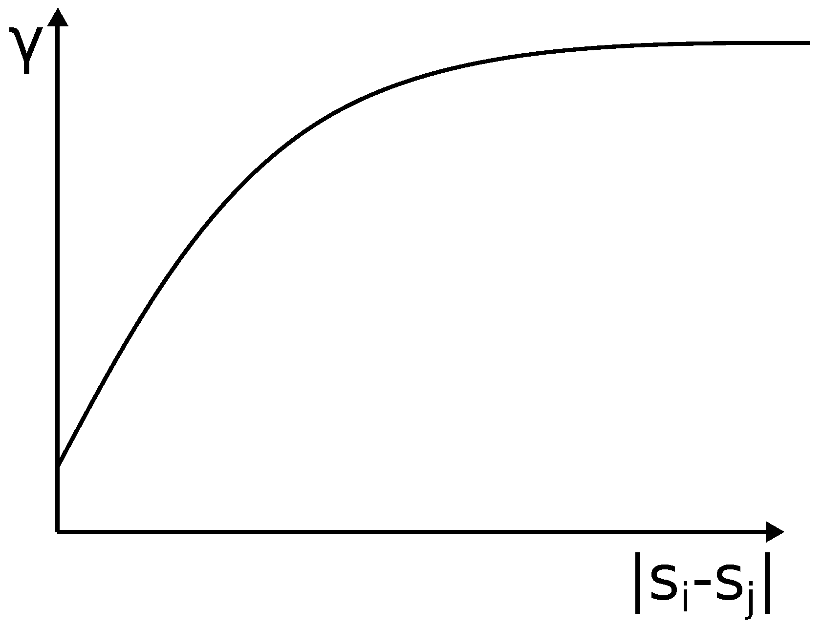
where is a weight corresponding to variable . To determine the , a function called variogram () is needed. One such variogram is depicted in Figure 5. Formally, variogram can be written as [205,206]:
Effectively, variogram indicates that the closer two points and are, the difference between their respective variables should be lower and vice versa. Using the variogram, weights can be determined by solving the matrix equation [207]:
or its transpose:
where w is the vector comprised of , T is the matrix comprised of and R is the matrix consisting of [207]. Naturally, the estimation may not only be carried out spatially but also temporally [205,206]. Interpolation-based methods are amongst the oldest methods to be utilised in gap-filling in satellite oceanography [100,109] and have remained somewhat popular throughout the years [38,47,54,57,60,64,67,73,76,83,86,99,108,110,111,112,113,117,120,121,132,140,152,153,154,157,158,162,163,164,191,193].
Figure 5.
A theoretical variogram. The further two points are, their correlation becomes less and less significant up until a final cutoff value.
Figure 5.
A theoretical variogram. The further two points are, their correlation becomes less and less significant up until a final cutoff value.
3.4. K-Nearest Neighbours
K-nearest neighbours (KNN) is a machine learning regression-solving method [208]. Regression takes form based on the sum of the K closest available data points. The sum can take many different forms, but it is most commonly expressed as a weighted function or as uniform [208]. In case of a weighted sum, increased distance equates to diminished influence. The distance is usually Euclidean, but if KNN is used in a geophysical domain, the distance may be the actual geographical distance [208]. Just like SVR, KNN is not overly popular [67,74,163,164], but as a part of machine-learning reconstruction, it is also noteworthy.
3.5. Random Forest/Decision Tree
Random Forest (RF) stems from the Decision Tree (DT) algorithm. Although primarily used for classification problems, RF exhibits a capacity for regression problems as well [209]. Starting with DT, let be a vector or a single point in data space. The vector components are then its features. DT functions by diving the data space into arbitrary classes according to various conditions based on the data features. With sufficiently enough conditions (so-called nodes), DT effectively divides the data space into enough classes so that each and every outcome of the nodes (so-called leaf) corresponds to an individual data point [209,210]. A simplified DT is depicted in Figure 6. RF is essentially made up of numerous DTs. Decisions made this way are the result of majority of decisions obtained from individual DTs. This improves stability and accuracy [209]. RF solves regression problems by first modelling a forest which accurately connects independent and target variables. Once the RF has been sufficiently trained, RF is provided with available independent variables and is tasked with determining the missing dependent variables [211].
3.6. Self-Organising Maps
Self-Organising Maps (SOM) is an unsupervised learning method typically used in classification problems [212]. However, it may be utilised for data reconstruction purposes [64]. SOM operates on neuron mesh, of a predetermined shape and structure [212]. The idea of SOM is as follows: let M denote a data manifold containing vectors v. This manifold can be described via the aforementioned mesh by moving the neurons (also known as Best Matching Units ), so that the distance between the individual BMUs and the vectors v is minimal [212]. Depending on the mesh, there are N available. Should the data vectors v be distributed by the probability distribution within the data manifold M, the reconstruction error L is given by:
Effectively, SOM functions by moving the BMUs through data space, reshaping the mesh to fit the manifold as closely as possible. However, since the BMUs are located on a “fixed” mesh, forming a strong correlation between individual s, so that moving one affects the neighbouring s [212]. The mesh often comes in a form of two-dimensional lattice [212]. Utilising this concept, SOM can be trained to describe typical oceanographic (or any other type of data) data manifolds by learning on complete datasets. Similarly to RF, once the model has been sufficiently trained, SOM can be used to predict the missing values based on available data [64,96,157], but unlike RF, SOM’s popularity is more akin to the popularity of SVR and KNN.
3.7. Neural Networks
Neural networks (NN) are a subsection of machine learning methods with wide applicability. Traditionally, NN are introduced by examining the perceptron model [213]. Perceptron is a function which intakes input variable x and outputs the output variable . One of the simpler transformations is:
where a is the weight, and b is bias [213]. After transformation, the output is compared to the desired output value y. Depending on this comparison, the weight is updated, and the process repeats itself until the error between and y is acceptable [213]. By combining these transformative functions in succession, deep neural networks are constructed [214,215]. The aforementioned functions now act as layers and can be grouped into the input layer, the output layer and the convoluted layer. The way the layers are ordered and organised is customisable, allowing for creation of various architectures of NN, such as Feed-forward NN [216] and Long Short-Term Memory [217]. Among these architectures are also the fairly new Generative Adversarial Networks (GAN) [218] and AutoEncoders (AE) [219].
3.7.1. Generative Adversarial Networks
GAN actually consists of two separate networks: a generating network, or the generator (G), and a discriminating network, or the discriminator (D). The aim of the generator is to generate a distribution to be as similar as possible to the distribution of real data x. For a given input z from distribution , the generator generates as output. Discriminator, on the other hand, has to determine whether originated from or . This decision comes in the form of scalar . Therefore, the discriminator aims to become as accurate as possible when discriminating between “real” and "generated" data, while the generator aims to generate data as similar as possible to “real” data [218]. Mathematically, this is a min-max optimisation of the so-called loss function [218]:
3.7.2. AutoEncoders
AE function on the principle of information bottleneck [219,220]. AE consists of three layers: the encoder, the bottleneck and the decoder. The idea behind AE is based on dimensionality reduction: reducing the number of features required for data description. The encoder e is tasked with determining the reduced dimensionality, so that [219,220]:
This way, point data x from n-dimensional data space is transcribed into m-dimensional latent data space . Effectively, the data are being encoded. Decoding of the data is achieved by the decoder d [219,220]:
which is nothing more than returning the data back into the original n-dimensional data space . Finally, the bottleneck is tasked with further reducing the dimension m, so that the final dimension of the latent data space is lower than needed for direct reconstruction. AE aims to reduce the difference [219,220]:
utilising the noise variable :
In terms of data reconstruction, takes shape of missing data. AutoEncoder is the basis of a popular reconstruction method called DINCAE: Data INterpolating Convolutional AutoEncoder [94,105]. Similarly to DINEOF, DINCAE effectively reduces dimensionality in the input data, but whereas DINEOF relied on EOF decomposition, DINCAE relies on the convolutional layers of the encoder and the bottleneck [105].
3.8. Data Merge and Other Reconstruction Methods
Apart from the listed methods, there are several other methods useful for reconstruction. Out of these, the most prominent is data merging—merging data from various sources [35,41,42,46,48,51,68,79,97,98,108,114,117,131,148,149,152,158]. Technically, this approach is better referred to as gap-filling, but for the purposes of this paper, data merging was still taken into consideration. The remainder of these methods refers to various numerical models, filters, composites, spatial scaling, etc. [29,32,36,53,80,103,116,118,126,129,136,138,141,145,155,156,157,192].
4. Summary Review of Reconstruction Methods in Literature
Presented in this section are more than 130 articles surveyed in preparation of this paper. During research, papers were selected by two criteria. The first criterion is that the paper has to feature any oceanographical satellite data. As mentioned earlier, these data mostly refer to and SST, but other types of oceanographic data are also considered. The second criterion is that the gaps in the obtained satellite data have to be filled using any viable method. This criterion includes articles that propose novel gap-filling methods—i.e., development articles, but also any article that fills gaps in the initially retrieved data before further analysing and processing the data in ways that do not necessarily have to deal with the issue of missing data reconstruction—i.e., application articles. Naturally, out of all the surveyed articles, more are classified as application articles than as development articles. The statistics of survey covering the source journals are presented in Appendix A. Considering the number of articles reviewed, it is impractical to thoroughly display all nuances of each and every one of them. Therefore, articles were surveyed in the most concise manner possible, extracting parameters relevant to the majority of the articles. Due to the sheer size of the findings, the resulting Table A1 is placed in Appendix B.
To illustrate the popularity of reconstruction methods throughout the years from Table A1, Figure 7a,b have been added. Methods have been grouped as defined in Section 2. While EOF-based methods are the most popular ones, during the past several years, NN-based (and machine-learning-based in general) methods started to be utilised more consistently and gained certain popularity.
Finally, to provide another useful point of view, surveyed articles have been cross-referenced against the three groups of data (, SST and other) and the nine groups of methods (EOF-based, SVR, interpolation-based, KNN, RF, SOM, NN, data merge and other). This cross-referencing is displayed in Table 2.
5. Discussion and Conclusions
Presented in this paper are more than 130 articles dealing with reconstruction of missing satellite oceanographic data. While this number of articles does not represent the entire effort of the scientific community, it does provide a representative insight into gap-filling methods. The survey provided several results. Firstly, seems to be the lead targeted type of variable in papers considered, with SST following. Other variables are of significantly lesser interest. From a data-level point of view, level 3 data are the most prominent, with individual swaths of data receiving some attention. Reconstruction at level 1 is significantly hindered as atmospheric correction plays a vital role in satellite observations. Regarding method popularity, DINEOF is undoubtedly the most popular reconstruction method: it is clear that reconstruction efforts in general started garnering ever-increasing attention only after the advent of DINEOF. While DINEOF has proven to be the gold standard, as demonstrated by the abundance in the univariate-time-series box of the novel approach categorisation system, the nearer future might witness a shift from EOF-based to machine-learning-based reconstructions. With the ever-growing and diverging sea of reconstruction methods, the proposed categorisation system might become an invaluable navigation tool amidst the chaos.
Author Contributions
Conceptualization, L.Ć., F.M. and H.K.; validation, L.Ć., F.M. and H.K.; formal analysis, L.Ć.; investigation, L.Ć.; resources, L.Ć.; writing—original draft preparation, L.Ć.; writing—review and editing, F.M. and H.K.; visualization, L.Ć.; supervision, F.M. and H.K; project administration, H.K.; funding acquisition, H.K. All authors have read and agreed to the published version of the manuscript.
Funding
This work has been supported in part by the Croatian Science Foundation under the project UIP-2019-04-1737.
Institutional Review Board Statement
Not applicable.
Informed Consent Statement
Not applicable.
Data Availability Statement
Not applicable.
Conflicts of Interest
The authors declare no conflict of interest. The funders had no role in the design of the study; in the collection, analyses, or interpretation of data; in the writing of the manuscript, or in the decision to publish the results.
Appendix A
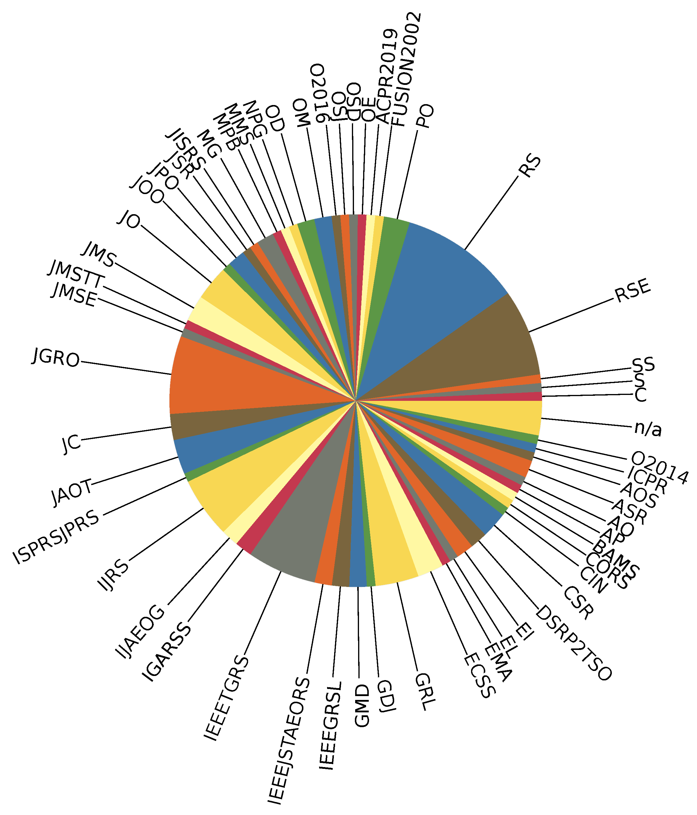
For the survey to be valid, the survey itself needs to be bias-free. Since the target of this survey are articles, it is prudent to verify two criteria: both publishing journals and years of publication must be represented as equally as possible. The inclusion of journals is represented in Figure A1, while the inclusion of publication years can be viewed in Figure 7a. Both statistics show that, in general, there is no strong bias towards any single journal or publication year; however, it can be noted that Remote Sensing and Remote Sensing Environment are slightly more popular than the rest of the journals, which should come as no surprise since they specialise in remote sensing and related issues. It is also clear that gap-filling interest rose sometime after 2005, coinciding with the development of DINEOF.
Figure A1.
Representation statistics regarding publishing journals of the surveyed articles. List of abbrevations: O2014—2014 Oceans St. John’s, OCEANS 2014, ICPR—2018 24th International Conference on Pattern Recognition, AOS—Acta Oceanologica Sinica, ASR—Advances in Space Research, AO—Applied Optics, AP—Aquatic Procedia, BAMS—Bulletin of the American Meteorological Society, CORS—Coastal Ocean Remote Sensing, CIN—Computational Intelligence and Neuroscience, CSR—Continental Shelf Research, DSRP2TSO—Deep Sea Research Part II: Topical Studies in Oceanography, EI—Ecological Indicators, EL—Ecology Letters, EMA—Environmental Monitoring and Assessment, ECSS—Estuarine, Coastal and Shelf Science, GRL—Geophysical Research Letters, GDJ—Geoscience Data Journal, GDM—Geoscientific Model Development, IEEEGRSL—IEEE Geoscience and Remote Sensing Letters, IEEEJSTAEORS—IEEE Journal of Selected Topics in Applied Earth Observations and Remote Sensing, IEEETGRS—Geoscience and Remote Sensing, IEEE Transactions, IGARSS—IGARSS 2019—2019 IEEE International Geoscience and Remote Sensing Symposium, IJAEOG—International Journal of Applied Earth Observation and Geoinformation, IJRS—International Journal of Remote Sensing, ISPRSJPRS—ISPRS Journal of Photogrammetry and Remote Sensing, JAOT—Journal of Atmospheric and Oceanic Technology, JC—Journal of Climate, JGRO—Journal of Geophysical Research: Oceans, JMSE—Journal of Marine Science and Engineering, JMSTT—Journal of Marine Science and Technology (Taiwan), JMS—Journal of Marine Systems, JO—Journal of Oceanography, JOO—Journal of Operational Oceanography, JPO—Journal of Physical Oceanography, JSR—Journal of Sea Research, JISRS—Journal of the Indian Society of Remote Sensing, MG—Marine Geodesy, MPB—Marine Pollution Bulletin, MMS—Mediter. Mar. Sci., NPG—Nonlinear Processes in Geophysics, OD—Ocean Dynamics, OM—Ocean Modelling, O2016—OCEANS 2016—Shanghai, OSJ—Ocean Science Journal, OSD—Ocean Science Discussions, OE—Opt. Express, ACPR2019—Pattern Recognition: 5th Asian Conference, ACPR 2019, FUSION2002—Proceedings of the Fifth International Conference on Information Fusion 2002, PO—Progress in Oceanography, RS—Remote Sensing, RSE—Remote Sensing of Environment, S—Science, SS—Spatial Statistics, C—The Cryosphere.

Appendix B
Presented in this Appendix is the Table A1 containing information obtained from over 130 surveyed articles. Information includes: reference, target data type, target data level, spatial and temporal resolution, reconstruction method, proxy data, reported accuracy of the reconstruction and the targeted region (If some information if not available or applicable for a given article, it will be displayed as n/a). Information in Table A1 is taken directly from the cite source. If the article provides multiple accuracies, the best accuracy has been selected. Accuracy measures are displayed as-is, and the definitions can be found in the cited article. Should the reader desire more details, they are referred directly to the source material.

Table A1.
Information obtained from the surveyed articles. Names are taken from references where applicable.
Table A1.
Information obtained from the surveyed articles. Names are taken from references where applicable.
| Target Data | Resolution | Proxy Data | Reported Accuracy | Area of Interest | ||||
|---|---|---|---|---|---|---|---|---|
| Ref. | Type | Level | Spat. | Temp. | Method | |||
| [59] | chla | L3 | n/a | 1 d | VConstruct DINEOF | n/a | VConstruct: DINEOF: | Georgia Strait |
| [72] | chla | L3 | 1 km | 8 d | DINEOF | n/a | seas around India | |
| [73] | chla | L3 | 4 km | 1 d | DINEOF spat.-temp. krig. | n/a | DINEOF: spatio-temporal kirging: | South China Sea |
| [74] | chla | L3 | 4 km | 8 d | KNN SVR RF NN DINEOF | n/a | KNN: SVR: RF: NN: DINEOF: | Caspian Sea |
| [70] | chla | L3 | 4 km | 1 d | DINCAE uni. DICAE multi. DINEOF uni. DINEOF multi. | SST | DINCAE uni.: DINCEA multi.: DINEOF uni.: DINEOF multi.: | Luzon Strait seas |
| [75] | chla | L3 | 9 km | 1 d | RF | SST SIC T2M PAR U-V wind bathymetry coord. time | Ross Sea | |
| [157] | chla | L3 | 4 km 4 km 9 km 9 km | 8 d 8 d 8 d 3 d | lin. temp. int. inv.-dist. weigh. int. ord. krig. spat.-temp. krig. DINEOF SOM ridge reg. (w/, w/o chla) RF (w/, w/o ) | SIC SST SLA cloud cover U-V wind | n/a | Beaufort Sea Chukchi Sea Tropical Atlantic Gulf of Mexico |
| [69] | chla | L3 | 4 km | 8 d | DINEOF | n/a | Arabian Sea | |
| [156] | chla | L3 | n/a | 1 d | coverage increase through algorithm refinement | Rrs(443) | n/a | global |
| [79] | L3 | 9 km | 1 d | DINEOF data merge | n/a | mean ratio reconstructed/original: | gobal oligothropic ocean global deep waters coastal and inland waters global ocean | |
| [62] | L3 | 1 km | 1 d | RF | CI Rrs(469) low-qlt |
RMSD = 12.98% | Yellow Sea East China Sea | |
| [50] |
chla | L2 | 1 km | 1 d | DINEOF VE-DINEOF | n/a | DINEOF: RMSE = 0.26 S-N = 7.1 DINEOF : RMSE = 0.008 S-N = 9.7 VE-DINEOF : RMSE = S-N = 1717 VE-DINEOF : RMSE = S-N = 137 | Bohai Bay |
| [81] | L3 | n/a | 1 d | DINEOF | n/a | RE = 0.54% | Arabian Sea | |
| [68] | L3 | 1 km 4 km | 1 d | data merge OI | in situ L | Atlantic merged: R2 = 0.82 Atlantic interpolated: Global merged: Global interpolated: | Atlantic global | |
| [46] | SST chla | L2 | 1 km | 1 d | data merge | num. model | SST: RMSE = 0.73 : | Baltic Sea |
| [67] | L3 | 4 km | 1 d | KNN lin. reg. log. reg. DT RF ET | SST SIC PAR T2M U-V wind bathymetry coord. time | poor acc. for the first 4 RF: R2 = 0.99 ET: | Ross Sea | |
| [134] | L3 | 4 km | 1 d | NN | SST atm. vapor wind rain rate cloud liquid | full model: R2 = 0.89 | Korean Peninsula | |
| [30] | chaa | L1 L3 | 9 km | 1 d | DINEOF | n/a | mean ratio reconstructed/original: daily: weekly: monthly: | global |
| [71] | L3 | 4 km | 8 d | DINEOF | n/a | RMSE = | Arabian Sea | |
| [135] | L3 | 1 km | 1 d 8 d | DINEOF | n/a | Year-to-year: daily: weekly: Complete span: daily: weekly: | Georgia Strait | |
| [85] | chla | L3 | 4.6 km | 8 d | DINEOF | n/a | n/a | SW Atlantic |
| [40] | L2 | 0.5 km | 1 d | DINEOF | n/a | mean ratio reconstructed/original: Bohai Sea: East China Sea: | Bohai Sea East China Sea | |
| [87] | chla SST PAR | L3 | 4 km | 8 d | DINEOF | n/a | Error: SST: < 1 PAR <2 chla < 0.2 | Iceland |
| [90] | chla SST | L3 | 4 km | 1 d | DINEOF multi. | SST | n/a | Gulf of Mexico |
| [65] | L3 | 9 km | 1 d | NN | SSH SSS SST ARGO S (salinity) ARGO T time coord. | RMSE = 0.091 | global | |
| [44] | chla SST | L2 | n/a | 1 d | DINEOF | n/a | n/a | Persian Gulf |
| [31] | L1 | 4 km (4 × 8 km) | 15" | DINEOF | n/a | n/a | North Sea | |
| [63] | L3 | 9 km | 1 w | DINEOF | n/a | Red Sea | ||
| [43] | chla SST | L2 | 1 km | 1 d | DINEOF | n/a | n/a | Peru/Chile |
| [88] | chla SST | L3 | 4 km | 1 d | DINEOF multi. | SST chla | RMSE = 0.157
seasonal cycle on/off | Georges Bank |
| [34] | L2 | 1 km | 1 d | DINEOF | n/a | n/a | South China Sea | |
| [36] | L2 | 4 km | 1 d | scale-changing climatology | low-qlt chla | n/a | N Atlantic | |
| [82] | L3 | 1 km | 1 d | DINEOF | n/a | n/a | Sicily Channel | |
| [66] | L3 | n/a | 1 m | DINEOF | n/a | RMSE = 0.11
| Bohai Sea Yellow Sea | |
| [78] | L3 | 9 km | 8 d | O-DINEOF S-DINEOF C-DINEOF D-DINEOF | n/a | O-DINEOF: SNR = 3.72 S-DINEOF: C-DINEOF: D-DINEOF: | Bohai Sea Yellow Sea | |
| [132] | L3 | 9 km | 8 d | interpolation padding | climatology | n/a | N Atlantic | |
| [91] | chla SST | L3 | 9 km | 8 d | DINEOF | n/a | n/a | Gulf of Alaska |
| [64] | L3 | 9 km | 1 d | SOM lin. interp. | SST SSH | daily DINEOF: RE = 0.25 weekly DINEOF: daily lin. int.: weekly lin. int.: | Mauritania | |
| [39] | L2 | 4.5 km | 1 d | DINEOF LSEOF RSEOF | n/a | n/a | Galapagos | |
| [92] | chla SST | L3 | 4 km | 1 d | DINEOF stat. model | SST SSH | DINEOF SST: R2 = 0.95/0.57 seasonal cycle on/off DINEOF / model: | Gulf of Mexico |
| [35] | L2 | 1 km 4 km | 1 d | data merge | n/a | n/a | California Coast | |
| [77] | L3 | 1 km | 8 d | DINEOF | n/a | R2 = 0.82 | Mediterranean Sea | |
| [58] | L3 | 9 km | 1 d | DINEOF | n/a | n/a | Peru–Chile | |
| [138] | chla SST MLD | L3 | 4.5 km | 8 d | GSM01 semi-anal. OC (Ocean Colour) model | n/a | n/a | Gulf of Cadiz |
| [86] | chla PAR | L3 | 9 km | 1 w | spat.-temp. int. | n/a | n/a | global |
| [52] | chla TSM SST | L2 | 1 km | 1 d | DINEOF | n/a | TMS min-max: R2 = 0.45 − 0.95 min-max: | English Channel |
| [195] | TSM SST TSM wind | n/a | n/a | n/a | DINEOF uni. DINEOF multi. | wind chla SST | n/a | English Channel Gulf of Mexico Mediterranean Sea Black Sea |
| [57] | L2 | 1 km | 1 d | kriging | n/a | (log) | Ireland Biscay Bay Iberia | |
| [95] | chla SST | L3 | 4 km | 1 d | DINEOF mulit. | chla SST | DINEOF SST: R2 = 0.93/0.53 seasonal cycle on/off | S Atlantic Bight |
| [194] | SST | n/a | 1 km | 1 d | DINEOF DINEOF Pruning OI | n/a | DINEOF: MSE = 0.086 DINEOF pruning: OI: | Tanganyika Lake |
| [53] | chla CDM | L2 | 1 km | 1 d | GSM01 semi-anal. OC model | R2 = 0.678 CDM: | global | |
| [42] | L2 | 2 km | 1 d | data merge | n/a | nL(412): R2 = 0.48 nL(440): nL(490/500): nL(551/555): nL(667/674): | Mediterranean Sea | |
| [80] | L3 | 1 d | turbulent cascading | n/a | n/a | global | ||
| [89] | chla SST | L3 | 4 km | 1 d | DINEOF multi. | SST | DINEOF SST: R2 = 0.97/0.69 seasonal cycle on/off | S Atlantic Bight |
| [60] | L3 | n/a | 1 m | spat. int. | n/a | n/a | N Atlantic | |
| [37] | L2 | n/a | 1 d | DINEOF | n/a | R2 = 0.912 | Adriatic Sea | |
| [83] | chla | L3 | 1 km | 1 d | spat.-temp. int. | n/a | n/a | Mississippi Bight |
| [41] | L2 | 1 km | 1 d | data merge | n/a | nL(412): nL(440): nL(500): nL(555): nL(675): | Adriatic Sea | |
| [38] | L2 | 1.5 km | 1 d | ord. krig. | n/a | n/a | North Sea | |
| [93] | chla SST wind | L3 | 1 km | 1 d | DINEOF uni. DINEOF multi. | chla SST wind | : SST: RMSE = 0.76 SST + wind: SST +: SST + day lag SST +: wind RMSE = 2.8 | West Florida Shelf |
| [76] | L3 | 1 km | 1 d | weigh. avg. OI | n/a | Weighted averaging: R2 = 0.47 Optimal interpolation: | Atlantic Ocean | |
| [136] | chla | L3 | 4.5 km 1 km | 1 d | GSM01 semi-anal. OC model | R2 = 0.943 | global | |
| [131] | L3 | n/a | 1 m | data merge | in situ | n/a | global | |
| [61] | L3 | 1 km | 1 d | CCGAN | SST SSH low- res. chla | SSIM = 0.9462 MSE = 0.004 RE = 0.039 | Adriatic Sea | |
| [51] | L2 | 1 km | 1 d | data merge DINEOF | n/a | Data merge: RMSE = 0.408 DINEOF: RMSE = 0.38 | Mexico | |
| [109] | SST | L3 | 1 | 1 d | OI | n/a | Data-to-guess-error: 1.25 | global |
| [193] | SST | n/a | 1.3 km | 1 d | DINEOF OI | n/a | DINEOF: cloud coverage: 40% 60% OI: similar 80% | Adriatic Sea |
| [107] | SST | L3 | 18 km | 8 d | DINEOF | n/a | n/a | Japan East Sea |
| [191] | SST | n/a | 4 km | 1 d | DINEOF OI | n/a | DINEOF: RMSE = 0.42 | Corsica |
| [111] | SST | L3 | 1.2 km 2 km | 1 d | OI | n/a | RMSE = 0.69–0.82 | Baltic Sea North Sea |
| [140] | SST | L3 | 1.2 km 1.5 km | 1 d | OI | n/a | RMSE = 0.78 | Baltic Sea North Sea |
| [123] | SST | L3 | 4 km | 1 m | NN | MSLP T2M wind CC dewpoint T | RMSE = 0.1–0.7 | Mediterranean Sea |
| [108] | SST | L3 | 4.5 km | 1 d | OI data merge | SIC | N-S ratio: 0.5-0.35 | global |
| [119] | SST | L3 | 1 km | 1 d | DINEOF | n/a | R2 = 0.98 mean diff: 0.243 | Gulf of Trieste |
| [128] | SST | L3 | 4.8 km | 1 d | DINEOF | n/a | Black Sea | |
| [47] | SST chla | L2 | 1 km | n/a | OI | n/a | SST: RE = 1.2% ABS = 0.29 : RE = 23% ABS = 0.56 | Black Sea |
| [127] | SST | L3 | 1 | 5 d | DINEOF EOF | n/a | DINEOF: RMSE = 0.91 EOF: RMSE = 0.82 | Yangtze River estuary |
| [110] | SST | L3 | 5 km | 1 d | kriging | n/a | BIAS = −0.285 STD = 0.68 | English Channel |
| [130] | TSM | L3 | n/a | 1 d | DINEOF | n/a | RE = 40% RMSE = 7.36 R2 = 0.75 | English Channel |
| [55] | SST | L2 | 1 km | 1 d | DINEOF | n/a | RMSE = 0.265 MAD = 0.396 R2 = 0.635 | Bay of Biscay |
| [158] | SSH | L3 | 2 " | 1 d | OI data merge | n/a | RMSE = 2 | global |
| [104] | SSH | L3 | 0.25 | 1 w | EOF | in situ | Pacific: mean R2 = 0.42 Global: | Pacific Ocean global |
| [54] | SST SSS | L2 | 1 km | 1 d | kriging | n/a | SST: ME = 0.3 MAE = 0.65 RMSE = 0.84 R2 = 0.99 SSS: ME = 0.85 MAE = 2.08 RMSE = 2.76 | Chesapeake Bay |
| [144] | SST | L3 | n/a | 1 d | DINEOF | n/a | Mediterranean Sea | |
| [101] | SSH | L3 | n/a | n/a | EOF | in situ | n/a | global |
| [125] | SST | L3 | 4 km | 1 m | DINEOF I-DINEOF | n/a | DINEOF: R2 = 0.9925 S-N = 9.7743 RMSE = 0.3144 MAD = 0.1680 I-DINEOF: S-N = 25.4548 RMSE = 0.1526 MAD = 0.1140 | South China Sea |
| [142] | SST | L3 | 4 km | 1 d | DINEOF I-DINEOF VE-DINEOF | n/a | DINEOF: R2 = 0.9943 S-N = 11.0682 RMSE = 0.2773 MAD = 0.1515 I-DINEOF: S-N = 17.1149 RMSE = 0.2215 MAD = 0.1631 VE-DINEOF: S-N = 19.9641 RMSE = 0.1303 MAD = 0.0155 | South China Sea |
| [143] | SST | L3 | 4 km | 1 d | DINEOF | n/a | BIAS = −0.34 RMSE = 0.37 R2 = 0.95 | South China Sea |
| [33] | SSS | L2 | 0.15 | 1 d | DINEOF | n/a | RMSE = 0.66 CMSE = 0.63 BIAS = 0.19 R2 = 0.73 | N-E Atlantic Ocean Mediterranean Sea |
| [147] | SST | L3 | 0.25 | 1 d | NN | n/a | 1 day: R2 RMSE = 0.62 MAE = 0.53 2 days: RMSE = 0.63 MAE = 0.54 3 days: RMSE = 0.65 MAE = 0.55 4 days: RMSE = 0.67 MAE = 0.56 5 days: RMSE = 0.69 MAE = 0.58 | Indian Ocean |
| [96] | sub. vel. | L3 | 0.25 | 1 d | SOM | SSH SST ARGO vel. | R2 = 0.956 RMSE = 2.8 MAE = 18 | Antarctic Ocean |
| [133] | L3 | 4 km | 1 d | DINEOF | n/a | MOIDS: RMSE = 0.38 R2 = 0.74 VIIRS: RMSE = 0.13 | Laizhou Bay | |
| [192] | SST | n/a | n/a | n/a | GAN Telea TV Patch-Match | n/a | GAN-1: PNAR = 0.1310 GAN-2: PNAR = 0.0862 Telea: PNAR = 0.0333 TV: PNAR = 0.166 Patch-Match: PNAR = 0.1085 | n/a |
| [122] | SST | L3 | 2 km | 1 d | GAN | n/a | avg. occlusion MSE: | Pacific Ocean |
| [115] | SST | L3 | 2 km | 1 d | GAN | n/a | avg. occlusion MSE: | N Pacific |
| [102] | SSH | L3 | 0.25 | 1 w | CSEOF | SST SLP | R2 = 0.79 | Indian Ocean |
| [105] | SST | L3 | 4 km | 1 d | DINCAE DINEOF | n/a | DINCAE: RMSE = 1.1362 CRMSE = 1.0879 BIAS = −0.3278 DINEOF: RMSE = 1.1676 CRMSE = 1.1102 BIAS = −0.3616 | Provencal basin |
| [155] | L3 | 4 km | 8 d | gridfill | n/a | R2 = 0.968 RMSE = 0.0586 | Yellow Sea | |
| [56] | SST | L2 | 1 km | 1 d | NN SVR RF | in situ coord. time cloud cover | NN: R2 RMSE = 0.91 MAE = 0.69 SVR: RMSE = 0.79 MAE = 0.59 RF: RMSE = 0.85 MAE = 0.64 | Arabian Sea Bay of Bengal |
| [124] | SST | L3 | 1 km | 1 d | GAN | n/a | AVG = 0.35 SVD = 0.67 MAE = 0.80 RMSPE = 10.36 | Yellow Sea |
| [163] | wind | L4 | 0.125 | 6 h | lin. reg. KNN DT NN | n/a | lin. reg.: Amp = 0.30 ± 0.39 Ang = 0.40 ± 8.74 KNN: Amp = 0.78 ± 0.67 Ang = 10.10 ± 17.54 DT: Amp = 0.85 ± 0.82 Ang = 11.12 ± 18.79 NN: Amp = 0.41 ± 0.46 Ang = 5.22 ± 10.58 | Adriatic Sea |
| [164] | wind | L4 | 0.5 | 6 h | lin. reg. KNN | n/a | lin. reg.: Amp =2.16 ± 1.55 Ang = 24.49 ± 30.75 KNN: Amp = 2.19 ± 1.59 Ang = 24.70 ± 31.98 | Mediterranean Sea |
| [148] | chla SPM | L3 | 750 m 300 m | 1 d | data merge DINEOF | n/a | : Mean ratio = 1.016 ± 0.222 Mean diff = −0.013 ± 0.543 K: Mean ratio = 1.012 ± 0.154 Mean diff = −0.008 ± 0.165 SPM: Mean ratio = 1.020 ± 0.205 Mean diff = −0.17 ± 0.485 | global |
| [106] | SST | L3 | 4 km 10 km | 1 d | DINCAE RF merge | coord. time | DINCAE: R2 = 0.99 BIAS = 0.02 RMSE = 0.75 rRMSE = 4.23 MAE = 0.55 RF: BIAS = 0.02 RMSE = 0.87 rRMSE = 4.41 MAE = 0.61 | NW Pacific |
| [94] | SST SSH | L3 | 4 km n/a (non- gridded) | 1 d | DINCAE | SST wind chla | SST: RMSE = 0.54 10thth SSH: n/a | Adriatic Sea Mediterranean Sea |
| [126] | SST | L3 | 1/20 | 1 d | Hidden Markov Model | n/a | n/a | China coastal waters |
| [129] | TIT (thin-ice thickness) | L3 | 1 km | 1 d | weig. feat. recon. | n/a | R2 = 0.81 RMSE = 2140 | Brunt Ice Shelf |
| [48] | SST | L2 | n/a | 1 m | data merge | n/a | R2 = 0.97 RMSE = 0.91 BIAS = −0.14 | Gulf of Mexico |
| [154] | SST | L3 | 1 km 1/4 | 1 d | OI | n/a | seas. cycle: R2 | Florida Bay |
| [151] | SST | L3 | n/a | 1 d | DINEOF | n/a | n/a | Adriatic Sea |
| [84] | chla | L3 | 4.5 km 9 km | 1 d | SVR merge | n/a | n/a | global |
| [137] | chla | L3 | 4.5 km 9 km | 1 d | NN merge | n/a | n/a | global |
| [97] | OC | L3 | n/a | 1 d | data merge | n/a | 58% coverage increase | global |
| [98] | OC | L3 | n/a | 1 d | data merge | n/a | 44% coverage increase | global |
| [153] | SST | L3 | 2.3 km | 1 d | interpolation | n/a | n/a | NW Atlantic |
| [100] | SLA | L3 | 6 km | 10 d | interpolation multiscale est. | n/a | RMSE = 4.90 ± 3.11 | Mediterranean Sea |
| [45] | chla TSM | L2 | 1 km | 1 d | DINEOF | n/a | : R2 RMSE = 0.13 TSM: RMSE = 0.05 | Ariake Sea |
| [162] | SST | L4 | 0.05 0.25 | 1 d | OI DINEOF analog data ass. | n/a | OI: RMSE = 0.45 ± 0.08 R2 = 0.76 ± 0.07 DINEOF: RMSE = 0.40 ± 0.07 = 0.83 ± 0.05 data ass.: RMSE = 0.31 ± 0.05 = 0.88 ± 0.02 | South Africa |
| [120] | SST | L3 | 1/20 | 1 d | OI analog data ass. DINEOF NN | n/a | OI: RMSE = 0.75 analog data ass.: RMSE = 0.45 DINEOF: RMSE = 0.54 NN: RMSE = 0.43 | South Africa |
| [139] | SSH | L3 | 0.2 | 10 d | NN | n/a | RMSE = 10–45 R2 = 0.99–0.45 | Mediterranean Sea |
| [112] | SST | L3 | 1.4 km | 1 d | OI | n/a | n/a | Gulf of Maine |
| [103] | SSH | L3 | 2.5 | 1 d | weigh. filter | n/a | n/a | global |
| [113] | SST | L3 | 6 km 2 km 1.6 km 25 km | 1 d | OI data merge | in situ | BIAS = 0.17 RMSE = 0.81 | California |
| [150] | SST | L3 | 1.1 km | 1 m | EOF forecast | n/a | n/a | Alboran Sea |
| [121] | SST | L3 | 9 km | 1 d | NN interpolation | n/a | NN: BIAS = −0.28 RMSE = 0.87 R2 interpolation: BIAS = −0.49 RMSE = 1.24 | W Mediterranean |
| [117] | SST | L3 | 0.088 0.125 0.167 0.25 | 1 d | OI data merge | n/a | n/a | global |
| [146] | SST | L3 | 0.5 | 1 d | corr. formula | SIC climat. S | n/a | N Atlantic |
| [116] | SST | L3 | 0.2 | 1 d | Kalman filter | n/a | n/a | N Atlantic |
| [114] | SST | L3 | 0.01 0.25 | 1 d | data merge | n/a | BIAS = −0.01 STD = 0.95 | Pacific Ocean |
| [32] | LSI (landfast sea-ice) | L1 | 1 km | 1 d | temp. comp. | n/a | n/a | Mertz Glacier Tongue |
| [152] | SST | L3 | 1 km 5 km 9 km 25 km | 1 d | data merge interpolation | SIC | RMSE = 0.3 BIAS = −0.2 | global |
| [149] | chla | L3 | n/a | 1 d | data merge | R | ratio: 1 ± 0.22 K ratio: 1.05 ± 0.15 | global |
| [29] | SSS | L1 L3 | 0.05 0.25 | 1 d 9 d | Non-Bayesian retrieval DINEOF multifractal fusion | SST | N.B.R.: RMSE = 0.35 DINEOF: RMSE = 0.54 M.F.: RMSE = 0.32 | N Atlantic Mediterranean Sea |
| [49] | SST | L2 | 1 km | 1 d | NN | RMSE = 4.46 R2 | seas around USA | |
| [141] | SST | L3 | 0.25 | 1 d | Hidden Markov Model | n/a | n/a | South Africa |
| [118] | SST | L3 | 0.05 0.25 | 1 d | Kelman filter | low. res. SST | n/a | Malvinas |
| [99] | SIC | L3 | 1 km | 1 d | spat. scaling | n/a | n/a | Svalbard archipelago |
| [145] | SST | L3 | 0.05 0.25 | 1 d | semivariogram model | low. res. SST | n/a | Malvinas |
References
- Belward, A.; Bourassa, M.; Dowell, M.; briggs, S.; Dolman, H.A.; Holmlund, K.; Husband, R.; Quegan, S.; Simmons, A.; Sloyan, B.; et al. The Global Observing System for Climate: Implementation Needs. 2016. Available online: https://public.wmo.int/en/resources/library/global-observing-system-climate-implementation-needs (accessed on 27 December 2022).
- IOCCG. Why Ocean Colour? The Societal Benefits of Ocean-Colour Technology; IOCCG: Dartmouth, NS, Canada, 2008. [Google Scholar] [CrossRef]
- Bojinski, S.; Verstraete, M.; Peterson, T.C.; Richter, C.; Simmons, A.; Zemp, M. The Concept of Essential Climate Variables in Support of Climate Research, Applications, and Policy. Bull. Am. Meteorol. Soc. 2014, 95, 1431–1443. [Google Scholar] [CrossRef]
- Steele, J.; Thorpe, S.; Turekian, K. Measurement Techniques, Platforms & Sensors: A Derivative of the Encyclopedia of Ocean Sciences; Elsevier: Chicago, IL, USA, 2009. [Google Scholar]
- Campbell, J.B.; Wynne, R.H. Introduction to Remote Sensing; Guilford Press: New York, NY, USA, 2011. [Google Scholar]
- Robinson, I.S. Discovering the Ocean from Space: The Unique Applications of Satellite Oceanography; Springer: Berlin, Germany, 2016. [Google Scholar]
- Gordon, H. Physical Principles of Ocean Color Remote Sensing; University of Miami: Coral Gables, FL, USA, 2019. [Google Scholar] [CrossRef]
- Coble, P. Marine Optical Biogeochemistry: The Chemistry of Ocean Color. Chem. Rev. 2007, 107, 402–418. [Google Scholar] [CrossRef] [PubMed]
- Strong, A.E.; McClain, E.P. Improved Ocean Surface Temperatures From Space—Comparisons With Drifting Buoys. Bull. Am. Meteorol. Soc. 1984, 65, 138–142. [Google Scholar] [CrossRef]
- McClain, E.P. Global sea surface temperatures and cloud clearing for aerosol optical depth estimates. Int. J. Remote Sens. 1989, 10, 763–769. [Google Scholar] [CrossRef]
- Joseph, G. Fundamentals of Remote Sensing, 2nd ed.; Universities Press: Hyderabad, India, 2005. [Google Scholar]
- Wylie, D.; Jackson, D.L.; Menzel, W.P.; Bates, J.J. Trends in Global Cloud Cover in Two Decades of HIRS Observations. J. Clim. 2005, 18, 3021–3031. [Google Scholar] [CrossRef]
- Wentz, F.J.; Gentemann, C.; Smith, D.; Chelton, D. Satellite Measurements of Sea Surface Temperature Through Clouds. Science 2000, 288, 847–850. [Google Scholar] [CrossRef]
- Ackerman, S.A.; Strabala, K.I.; Menzel, W.P.; Frey, R.A.; Moeller, C.C.; Gumley, L.E. Discriminating clear sky from clouds with Modis. J. Geophys. Res. Atmos. 1998, 103, 32141–32157. [Google Scholar] [CrossRef]
- Wang, M.; Shi, W. Cloud Masking for Ocean Color Data Processing in the Coastal Regions. Geosci. Remote Sens. IEEE Trans. 2006, 44, 3105–3196. [Google Scholar] [CrossRef]
- Wang, M.; Bailey, S.W. Correction of sun glint contamination on the SeaWiFS ocean and atmosphere products. Appl. Opt. 2001, 40, 4790–4798. [Google Scholar] [CrossRef]
- Reynolds, R.W.; Folland, C.K.; Parker, D.E. Biases in satellite-derived sea-surface-temperature data. Nature 1989, 341, 728–731. [Google Scholar] [CrossRef]
- Reynolds, R.W. Impact of Mount Pinatubo Aerosols on Satellite-derived Sea Surface Temperatures. J. Clim. 1993, 6, 768–774. [Google Scholar] [CrossRef]
- Sathyendranath, S.; Brewin, R.J.; Brockmann, C.; Brotas, V.; Calton, B.; Chuprin, A.; Cipollini, P.; Couto, A.B.; Dingle, J.; Doerffer, R.; et al. An Ocean-Colour Time Series for Use in Climate Studies: The Experience of the Ocean-Colour Climate Change Initiative (OC-CCI). Sensors 2019, 19, 4285. [Google Scholar] [CrossRef]
- Meister, G.; McClain, C.R. Point-spread function of the ocean color bands of the Moderate Resolution Imaging Spectroradiometer on Aqua. Appl. Opt. 2010, 49, 6276–6285. [Google Scholar] [CrossRef]
- Varnai, T.; Marshak, A. Effect of Cloud Fraction on Near-Cloud Aerosol Behavior in the MODIS Atmospheric Correction Ocean Color Product. Remote Sens. 2015, 7, 5283–5299. [Google Scholar] [CrossRef]
- Hu, C.; Feng, L.; Lee, Z.; Davis, C.O.; Mannino, A.; McClain, C.R.; Franz, B.A. Dynamic range and sensitivity requirements of satellite ocean color sensors: Learning from the past. Appl. Opt. 2012, 51, 6045–6062. [Google Scholar] [CrossRef]
- NASA Ocean Color–SST. Available online: https://oceancolor.gsfc.nasa.gov/docs/modis_sst/ (accessed on 27 December 2022).
- Rajeesh, R.; Dwarakish, G. Satellite Oceanography—A review. Aquat. Procedia 2015, 4, 165–172. [Google Scholar] [CrossRef]
- Traon, P.Y.L.; Antoine, D.; Bentamy, A.; Bonekamp, H.; Breivik, L.; Chapron, B.; Corlett, G.; Dibarboure, G.; DiGiacomo, P.; Donlon, C.; et al. Use of satellite observations for operational oceanography: Recent achievements and future prospects. J. Oper. Oceanogr. 2015, 8, s12–s27. [Google Scholar] [CrossRef]
- NASA Ocean Color. Available online: https://oceancolor.gsfc.nasa.gov/ (accessed on 27 December 2022).
- Monitoring the Weather and Climate from Space. Available online: https://www.eumetsat.int/ (accessed on 27 December 2022).
- What’s behind the curtain of the NASA Plankton, Aerosol, Cloud, ocean Ecosystem (PACE) mission? Training Activity. Available online: https://www.us-ocb.org/wp-content/uploads/sites/43/2022/08/L14_PACE_Applications_PACECLASS_20220805.pdf/ (accessed on 27 December 2022).
- Olmedo, E.; Taupier-Letage, I.; Turiel, A.; Alvera-Azcárate, A. Improving SMOS Sea Surface Salinity in the Western Mediterranean Sea through Multivariate and Multifractal Analysis. Remote Sens. 2018, 10, 485. [Google Scholar] [CrossRef] [Green Version]
- Liu, X.; Wang, M. Gap Filling of Missing Data for VIIRS Global Ocean Color Products Using the DINEOF Method. IEEE Trans. Geosci. Remote Sens. 2018, 56, 4464–4476. [Google Scholar] [CrossRef]
- Alvera-Azcárate, A.; Vanhellemont, Q.; Ruddick, K.; Barth, A.; Beckers, J.M. Analysis of high frequency geostationary ocean colour data using DINEOF. Estuar. Coast. Shelf Sci. 2015, 159, 28–36. [Google Scholar] [CrossRef]
- Fraser, A.; Massom, R.; Michael, K. A Method for Compositing Polar MODIS Satellite Images to Remove Cloud Cover for Landfast Sea-Ice Detection. Geosci. Remote Sens. IEEE Trans. 2009, 47, 3272–3282. [Google Scholar] [CrossRef]
- Alvera-Azcárate, A.; Barth, A.; Parard, G.; Beckers, J.M. Analysis of SMOS sea surface salinity data using DINEOF. Remote Sens. Environ. 2016, 180, 137–145. [Google Scholar] [CrossRef]
- Liu, M.; Liu, X.; Ma, A.; Li, T.; Du, Z. Spatio-temporal stability and abnormality of chlorophyll-a in the Northern South China Sea during 2002–2012 from MODIS images using wavelet analysis. Cont. Shelf Res. 2014, 75, 15–27. [Google Scholar] [CrossRef]
- Kahru, M.; Kudela, R.M.; Manzano-Sarabia, M.; Greg Mitchell, B. Trends in the surface chlorophyll of the California Current: Merging data from multiple ocean color satellites. Deep Sea Res. Part II Top. Stud. Oceanogr. 2012, 77–80, 89–98. [Google Scholar] [CrossRef]
- Land, P.; Shutler, J.; Platt, T.; Racault, M. A novel method to retrieve oceanic phytoplankton phenology from satellite data in the presence of data gaps. Ecol. Indic. 2014, 37, 67–80. [Google Scholar] [CrossRef]
- Mauri, E.; Poulain, P.M.; Južnič-Zonta, V. MODIS chlorophyll variability in the northern Adriatic Sea and relationship with forcing parameters. J. Geophys. Res. Ocean. 2007, 112. [Google Scholar] [CrossRef]
- Müller, D. Estimation of Algae Concentration in Cloud Covered Scenes Using Geostatistical Methods; GKSS: Geesthacht, Germany, 2007. [Google Scholar]
- Taylor, M.H.; Losch, M.; Wenzel, M.; Schröter, J. On the Sensitivity of Field Reconstruction and Prediction Using Empirical Orthogonal Functions Derived from Gappy Data. J. Clim. 2013, 26, 9194–9205. [Google Scholar] [CrossRef]
- Liu, X.; Wang, M. Analysis of ocean diurnal variations from the Korean Geostationary Ocean Color Imager measurements using the DINEOF method. Estuar. Coast. Shelf Sci. 2016, 180, 230–241. [Google Scholar] [CrossRef]
- Mélin, F.; Zibordi, G. Optically based technique for producing merged spectra of water-leaving radiances from ocean color remote sensing. Appl. Opt. 2007, 46, 3856–3869. [Google Scholar] [CrossRef]
- Mélin, F.; Zibordi, G.; Djavidnia, S. Merged series of normalized water leaving radiances obtained from multiple satellite missions for the Mediterranean Sea. Adv. Space Res. 2009, 43, 423–437. [Google Scholar] [CrossRef]
- Corredor Acosta, A.; Morales, C.; Hormazabal, S.; Andrade, I.; Correa-Ramirez, M. Phytoplankton phenology in the coastal upwelling region off central-southern Chile (35 ∘S–38 ∘S): Time-space variability, coupling to environmental factors, and sources of uncertainty in the estimates. J. Geophys. Res. Ocean. 2015, 120, 813–831. [Google Scholar] [CrossRef]
- Moradi, M.; Kabiri, K. Spatio-temporal variability of SST and Chlorophyll-a from MODIS data in the Persian Gulf. Mar. Pollut. Bull. 2015, 98, 14–25. [Google Scholar] [CrossRef]
- Yang, M.; Khan, F.A.; Tian, H.; Liu, Q. Analysis of the Monthly and Spring-Neap Tidal Variability of Satellite Chlorophylla and Total Suspended Matter in a Turbid Coastal Ocean Using the DINEOF Method. Remote Sens. 2021, 13, 632. [Google Scholar] [CrossRef]
- Konik, M.; Kowalewski, M.; Bradtke, K.; Darecki, M. The operational method of filling information gaps in satellite imagery using numerical models. Int. J. Appl. Earth Obs. Geoinf. 2019, 75, 68–82. [Google Scholar] [CrossRef]
- Pukhtyar, L.D.; Stanichny, S.V.; Timchenko, I.E. Optimal interpolation of the data of remote sensing of the sea surface. Phys. Oceanogr. 2009, 19, 225. [Google Scholar] [CrossRef]
- Barnes, B.B.; Hu, C. A Hybrid Cloud Detection Algorithm to Improve MODIS Sea Surface Temperature Data Quality and Coverage Over the Eastern Gulf of Mexico. IEEE Trans. Geosci. Remote Sens. 2013, 51, 3273–3285. [Google Scholar] [CrossRef]
- Wang, J.; Deng, Z. Development of MODIS data-based algorithm for retrieving sea surface temperature in coastal waters. Environ. Monit. Assess. 2017, 189, 286. [Google Scholar] [CrossRef]
- Ping, B.; Meng, Y. Reconstruct Oceanic Chlorophyll and Reflectance Data Based on an Improved VE-DINEOF Method. In Proceedings of the IGARSS 2019—2019 IEEE International Geoscience and Remote Sensing Symposium, Yokohama, Japan, 28 July–2 August 2019; pp. 7984–7987. [Google Scholar] [CrossRef]
- Lomelı-Huerta, J.R.; Rivera-Caicedo, J.P.; De-la Torre, M.; Acevedo-Juárez, B.; Cepeda-Morales, J.; Avila-George, H. An approach to fill in missing data from satellite imagery using data-intensive computing and DINEOF. PeerJ Comput. Sci. 2022, 8, e979. [Google Scholar] [CrossRef]
- Sirjacobs, D.; Alvera-Azcárate, A.; Barth, A.; Lacroix, G.; Park, Y.; Nechad, B.; Ruddick, K.; Beckers, J.M. Cloud filling of ocean colour and sea surface temperature remote sensing products over the Southern North Sea by the Data Interpolating Empirical Orthogonal Functions methodology. J. Sea Res. 2011, 65, 114–130. [Google Scholar] [CrossRef]
- Maritorena, S.; d’Andon, O.H.F.; Mangin, A.; Siegel, D.A. Merged satellite ocean color data products using a bio-optical model: Characteristics, benefits and issues. Remote Sens. Environ. 2010, 114, 1791–1804. [Google Scholar] [CrossRef]
- Urquhart, E.A.; Hoffman, M.J.; Murphy, R.R.; Zaitchik, B.F. Geospatial interpolation of MODIS-derived salinity and temperature in the Chesapeake Bay. Remote Sens. Environ. 2013, 135, 167–177. [Google Scholar] [CrossRef]
- Ganzedo, U.; Alvera-Azcárate, A.; Esnaola, G.; Ezcurra, A.; Sáenz, J. Reconstruction of sea surface temperature by means of DINEOF: A case study during the fishing season in the Bay of Biscay. Int. J. Remote Sens. 2011, 32, 933–950. [Google Scholar] [CrossRef]
- Sunder, S.; Ramsankaran, R.; Ramakrishnan, B. Machine learning techniques for regional scale estimation of high-resolution cloud-free daily sea surface temperatures from MODIS data. ISPRS J. Photogramm. Remote Sens. 2020, 166, 228–240. [Google Scholar] [CrossRef]
- Saulquin, B.; Gohin, F.; Garrello, R. Regional Objective Analysis for Merging High-Resolution MERIS, MODIS/Aqua, and SeaWiFS Chlorophyll-a Data From 1998 to 2008 on the European Atlantic Shelf. IEEE Trans. Geosci. Remote Sens. 2011, 49, 143–154. [Google Scholar] [CrossRef]
- Correa-Ramirez, M.A.; Hormazabal, S.E.; Morales, C.E. Spatial patterns of annual and interannual surface chlorophyll-a variability in the Peru–Chile Current System. Prog. Oceanogr. 2012, 92–95, 8–17. [Google Scholar] [CrossRef]
- Ehrler, M.; Ernst, N. VConstruct: Filling Gaps in Chl-a Data Using a Variational Autoencoder. arXiv 2021, arXiv:2101.10260. [Google Scholar] [CrossRef]
- Beaugrand, G.; Edwards, M.; Brander, K.; Luczak, C.; Ibanez, F. Causes and projections of abrupt climate-driven ecosystem shifts in the North Atlantic. Ecol. Lett. 2008, 11, 1157–1168. [Google Scholar] [CrossRef]
- Ćatipović, L.; Kalinić, H.; Županović, T.; Sathyendranath, S.; Dingle, J.; Jackson, T.; Matić, F. Implementation of GAN-based satellite derived chlorophyll-a concentration gap reconstruction. 2023; manuscript submitted for publication. [Google Scholar]
- Chen, S.; Hu, C.; Barnes, B.B.; Xie, Y.; Lin, G.; Qiu, Z. Improving ocean color data coverage through machine learning. Remote Sens. Environ. 2019, 222, 286–302. [Google Scholar] [CrossRef]
- Dreano, D.; Mallick, B.; Hoteit, I. Filtering remotely sensed chlorophyll concentrations in the Red Sea using a space–time covariance model and a Kalman filter. Spat. Stat. 2015, 13, 1–20. [Google Scholar] [CrossRef]
- Jouini, M.; Levy, M.; Crépon, M.; Thiria, S. Reconstruction of satellite chlorophyll images under heavy cloud coverage using a neural classification method. Remote Sens. Environ. 2013, 131, 232–246. [Google Scholar] [CrossRef]
- Krasnopolsky, V.; Nadiga, S.; Mehra, A.; Bayler, E.; Behringer, D. Neural networks technique for filling gaps in satellite measurements: Application to ocean color observations. Comput. Intell. Neurosci. 2016, 2016, 1–9. [Google Scholar] [CrossRef] [PubMed]
- Liu, D.; Wang, Y. Trends of satellite derived chlorophyll-a (1997–2011) in the Bohai and Yellow Seas, China: Effects of bathymetry on seasonal and inter-annual patterns. Prog. Oceanogr. 2013, 116, 154–166. [Google Scholar] [CrossRef]
- Park, J.; Kim, J.H.; Kim, H.C.; Kim, B.K.; Bae, D.; Jo, Y.H.; Jo, N.; Lee, S.H. Reconstruction of Ocean Color Data Using Machine Learning Techniques in Polar Regions: Focusing on Off Cape Hallett, Ross Sea. Remote Sens. 2019, 11, 1366. [Google Scholar] [CrossRef]
- Saulquin, B.; Gohin, F.; d’Andon, O.F. Interpolated fields of satellite-derived multi-algorithm chlorophyll-a estimates at global and European scales in the frame of the European Copernicus-Marine Environment Monitoring Service. J. Oper. Oceanogr. 2019, 12, 47–57. [Google Scholar] [CrossRef]
- Shunmugapandi, R.; Inamdar, A.B.; Gedam, S.K. Long-time-scale investigation of phytoplankton communities based on their size in the Arabian Sea. Int. J. Remote Sens. 2020, 41, 5992–6009. [Google Scholar] [CrossRef]
- Han, Z.; He, Y.; Liu, G.; Perrie, W. Application of DINCAE to Reconstruct the Gaps in Chlorophyll-a Satellite Observations in the South China Sea and West Philippine Sea. Remote Sens. 2020, 12, 480. [Google Scholar] [CrossRef]
- Jayaram, C.; Priyadarshi, N.; Kumar, J.P.; Bhaskar, T.V.S.U.; Raju, D.; Kochuparampil, A.J. Analysis of gap-free chlorophyll-a data from MODIS in Arabian Sea, reconstructed using DINEOF. Int. J. Remote Sens. 2018, 39, 7506–7522. [Google Scholar] [CrossRef]
- Jayaram, C.; Jonnakuti, P.; Udaya Bhaskar, T.; Bhavani, I.; Rao, T.; Nagamani, P. Reconstruction of Gap-Free OCM-2 Chlorophyll-a Concentration Using DINEOF. J. Indian Soc. Remote Sens. 2021, 49, 1419–1425. [Google Scholar] [CrossRef]
- Mohamed Yussof, F.N. Reconstruction of chlorophyll-a data by using DINEOF approach in Sepanggar Bay, Malaysia. Comput. Sci. 2021, 16, 345–356. [Google Scholar]
- Mohebzadeh, H.; Mokari, E.; Daggupati, P.; Biswas, A. A machine learning approach for spatiotemporal imputation of MODIS chlorophyll-a. Int. J. Remote Sens. 2021, 42, 7381–7404. [Google Scholar] [CrossRef]
- Park, J.; Kim, H.C.; Bae, D.; Jo, Y.H. Data Reconstruction for Remotely Sensed Chlorophyll-a Concentration in the Ross Sea Using Ensemble-Based Machine Learning. Remote Sens. 2020, 12, 11898. [Google Scholar] [CrossRef]
- Pottier, C.; Garçon, V.; Larnicol, G.; Sudre, J.; Schaeffer, P.; Le Traon, P.-Y. Merging SeaWiFS and MODIS/Aqua Ocean Color Data in North and Equatorial Atlantic Using Weighted Averaging and Objective Analysis. IEEE Trans. Geosci. Remote. Sens. 2006, 44, 3436–3451. [Google Scholar] [CrossRef]
- Volpe, G.; Nardelli, B.B.; Cipollini, P.; Santoleri, R.; Robinson, I.S. Seasonal to interannual phytoplankton response to physical processes in the Mediterranean Sea from satellite observations. Remote Sens. Environ. 2012, 117, 223–235. [Google Scholar] [CrossRef]
- Wang, Y.; Liu, D. Reconstruction of satellite chlorophyll-a data using a modified DINEOF method: A case study in the Bohai and Yellow seas, China. Int. J. Remote Sens. 2014, 35, 204–217. [Google Scholar] [CrossRef]
- Liu, X.; Wang, M. Filling the Gaps of Missing Data in the Merged VIIRS SNPP/NOAA-20 Ocean Color Product Using the DINEOF Method. Remote Sens. 2019, 11, 178. [Google Scholar] [CrossRef]
- Pottier, C.; Turiel, A.; Garçon, V. Inferring missing data in satellite chlorophyll maps using turbulent cascading. Remote Sens. Environ. 2008, 112, 4242–4260. [Google Scholar] [CrossRef]
- Rebekah, S.; Inamdar, A.; Gedam, S.S. Long-Time-Scale Investigation of Phytoplankton Biomass Through Reconstructed Chlorophyll-A Data Using DINEOF Method. In Proceedings of the IGARSS 2019—2019 IEEE International Geoscience and Remote Sensing Symposium, Yokohama, Japan, 28 July–2 August 2019; pp. 7995–7998. [Google Scholar] [CrossRef]
- Rinaldi, E.; Buongiorno Nardelli, B.; Volpe, G.; Santoleri, R. Chlorophyll distribution and variability in the Sicily Channel (Mediterranean Sea) as seen by remote sensing data. Cont. Shelf Res. 2014, 77, 61–68. [Google Scholar] [CrossRef]
- Casey, B.; Arnone, R.; Flynn, P. Simple and efficient technique for spatial/temporal composite imagery. In Proceedings of the Coastal Ocean Remote Sensing; Frouin, R.J., Lee, Z., Eds.; International Society for Optics and Photonics—SPIE: Bellingham, WA, USA, 2007; Volume 6680, p. 668014. [Google Scholar] [CrossRef]
- Kwiatkowska, E.; Fargion, G. Application of machine-learning techniques toward the creation of a consistent and calibrated global chlorophyll concentration baseline dataset using remotely sensed ocean color data. Geosci. Remote Sens. IEEE Trans. 2004, 41, 2844–2860. [Google Scholar] [CrossRef]
- Andreo, V.C.; Dogliotti, A.I.; Tauro, C.B. Remote Sensing of Phytoplankton Blooms in the Continental Shelf and Shelf-Break of Argentina: Spatio-Temporal Changes and Phenology. IEEE J. Sel. Top. Appl. Earth Obs. Remote Sens. 2016, 9, 5315–5324. [Google Scholar] [CrossRef]
- Racault, M.F.; Le Quéré, C.; Buitenhuis, E.; Sathyendranath, S.; Platt, T. Phytoplankton phenology in the global ocean. Ecol. Indic. 2012, 14, 152–163. [Google Scholar] [CrossRef]
- McGinty, N.; Guðmundsson, K.; Ágústsdóttir, K.; Marteinsdóttir, G. Environmental and climactic effects of chlorophyll-a variability around Iceland using reconstructed satellite data fields. J. Mar. Syst. 2016, 163, 31–42. [Google Scholar] [CrossRef]
- Li, Y.; He, R. Spatial and temporal variability of SST and ocean color in the Gulf of Maine based on cloud-free SST and chlorophyll reconstructions in 2003–2012. Remote Sens. Environ. 2014, 144, 98–108. [Google Scholar] [CrossRef]
- Miles, T.N.; He, R.; Li, M. Characterizing the South Atlantic Bight seasonal variability and cold-water event in 2003 using a daily cloud-free SST and chlorophyll analysis. Geophys. Res. Lett. 2009, 36. [Google Scholar] [CrossRef]
- Shropshire, T.; Li, Y.; He, R. Storm impact on sea surface temperature and chlorophyll a in the Gulf of Mexico and Sargasso Sea based on daily cloud-free satellite data reconstructions. Geophys. Res. Lett. 2016, 43, 12199–12207. [Google Scholar] [CrossRef]
- Waite, J.N.; Mueter, F.J. Spatial and temporal variability of chlorophyll-a concentrations in the coastal Gulf of Alaska, 1998–2011, using cloud-free reconstructions of SeaWiFS and MODIS-Aqua data. Prog. Oceanogr. 2013, 116, 179–192. [Google Scholar] [CrossRef]
- Zhao, Y.; He, R. Cloud-free sea surface temperature and colour reconstruction for the Gulf of Mexico: 2003–2009. Remote Sens. Lett. 2012, 3, 697–706. [Google Scholar] [CrossRef]
- Alvera-Azcárate, A.; Barth, A.; Beckers, J.M.; Weisberg, R.H. Multivariate reconstruction of missing data in sea surface temperature, chlorophyll, and wind satellite fields. J. Geophys. Res. Ocean. 2007, 112. [Google Scholar] [CrossRef]
- Barth, A.; Alvera-Azcárate, A.; Troupin, C.; Beckers, J.M. DINCAE 2.0: Multivariate convolutional neural network with error estimates to reconstruct sea surface temperature satellite and altimetry observations. Geosci. Model Dev. 2022, 15, 2183–2196. [Google Scholar] [CrossRef]
- Miles, T.N.; He, R. Temporal and spatial variability of Chl-a and SST on the South Atlantic Bight: Revisiting with cloud-free reconstructions of MODIS satellite imagery. Cont. Shelf Res. 2010, 30, 1951–1962. [Google Scholar] [CrossRef]
- Chapman, C.; Charantonis, A.A. Reconstruction of Subsurface Velocities From Satellite Observations Using Iterative Self-Organizing Maps. IEEE Geosci. Remote Sens. Lett. 2017, 14, 617–620. [Google Scholar] [CrossRef]
- Gregg, W.; Esaias, W.; Feldman, G.; Frouin, R.; Hooker, S.; McClain, C.; Woodward, R. Coverage opportunities for global ocean color in a multimission era. IEEE Trans. Geosci. Remote Sens. 1998, 36, 1620–1627. [Google Scholar] [CrossRef]
- Gregg, W.; Woodward, R. Improvements in coverage frequency of ocean color: Combining data from SeaWiFS and MODIS. IEEE Trans. Geosci. Remote Sens. 1998, 36, 1350–1353. [Google Scholar] [CrossRef]
- Preußer, A.; Willmes, S.; Heinemann, G.; Paul, S. Thin-ice dynamics and ice production in the Storfjorden polynya for winter seasons 2002/2003–2013/2014 using MODIS thermal infrared imagery. Cryosphere 2015, 9, 1063–1073. [Google Scholar] [CrossRef]
- Fieguth, P.; Menemenlis, D.; Ho, T.; Willsky, A.; Wunsch, C. Mapping Mediterranean Altimeter Data with a Multiresolution Optimal Interpolation Algorithm. J. Atmos. Ocean. Technol. 1998, 15, 535–546. [Google Scholar] [CrossRef]
- Hamlington, B.; Leben, R.; Strassburg, M.; Kim, K.Y. Cyclostationary empirical orthogonal function sea-level reconstruction. Geosci. Data J. 2014, 1, 13–19. [Google Scholar] [CrossRef]
- Kumar, P.; Hamlington, B.; Cheon, S.H.; Han, W.; Thompson, P. 20th Century Multivariate Indian Ocean Regional Sea Level Reconstruction. J. Geophys. Res. Ocean. 2020, 125, e2020JC016270. [Google Scholar] [CrossRef]
- Chambers, D.P.; Mehlhaff, C.A.; Urban, T.J.; Fujii, D.; Nerem, R.S. Low-frequency variations in global mean sea level: 1950–2000. J. Geophys. Res. Ocean. 2002, 107, 1-1–1-10. [Google Scholar] [CrossRef]
- Hamlington, B.D.; Leben, R.R.; Wright, L.A.; Kim, K.Y. Regional Sea Level Reconstruction in the Pacific Ocean. Mar. Geod. 2012, 35, 98–117. [Google Scholar] [CrossRef]
- Barth, A.; Alvera-Azcárate, A.; Licer, M.; Beckers, J.M. DINCAE 1.0: A convolutional neural network with error estimates to reconstruct sea surface temperature satellite observations. Geosci. Model Dev. 2020, 13, 1609–1622. [Google Scholar] [CrossRef]
- Jung, S.; Yoo, C.; Im, J. High-Resolution Seamless Daily Sea Surface Temperature Based on Satellite Data Fusion and Machine Learning over Kuroshio Extension. Remote Sens. 2022, 14, 575. [Google Scholar] [CrossRef]
- Park, S.; Chu, P. Interannual SST variability in the Japan/East Sea and relationship with environmental variables. J. Oceanogr. 2006, 62, 115–132. [Google Scholar] [CrossRef]
- Reynolds, R.W.; Smith, T.M.; Liu, C.; Chelton, D.B.; Casey, K.S.; Schlax, M.G. Daily High-Resolution-Blended Analyses for Sea Surface Temperature. J. Clim. 2007, 20, 5473–5496. [Google Scholar] [CrossRef]
- Reynolds, R.W.; Smith, T.M. Improved Global Sea Surface Temperature Analyses Using Optimum Interpolation. J. Clim. 1994, 7, 929–948. [Google Scholar] [CrossRef]
- Saulquin, B.; Gohin, F. Mean seasonal cycle and evolution of the sea surface temperature from satellite and in situ data in the English Channel for the period 1986–2006. Int. J. Remote Sens. 2010, 31, 4069–4093. [Google Scholar] [CrossRef]
- She, J.; Høyer, J.L.; Larsen, J. Assessment of sea surface temperature observational networks in the Baltic Sea and North Sea. J. Mar. Syst. 2007, 65, 314–335. [Google Scholar] [CrossRef]
- Bisagni, J.; Seemann, K.; Mavor, T. High-resolution satellite-derived sea-surface temperature variability over the Gulf of Maine and Georges Bank region, 1993–1996. Deep Sea Res. Part II Top. Stud. Oceanogr. 2001, 48, 71–94. [Google Scholar] [CrossRef]
- Chao, Y.; Li, Z.; Farrara, J.D.; Hung, P. Blending Sea Surface Temperatures from Multiple Satellites and In Situ Observations for Coastal Oceans. J. Atmos. Ocean. Technol. 2009, 26, 1415–1426. [Google Scholar] [CrossRef]
- Guan, L.; Kawamura, H. Merging Satellite Infrared and Microwave SSTs: Methodology and Evaluation of the New SST. J. Oceanogr. 2004, 60, 905–912. [Google Scholar] [CrossRef]
- Hirahara, N.; Sonogashira, M.; Kasahara, H.; Iiyama, M. Denoising and Inpainting of Sea Surface Temperature Image with Adversarial Physical Model Loss. In Proceedings of the Pattern Recognition: 5th Asian Conference, ACPR 2019, Auckland, New Zealand, 26–29 November 2019; Revised Selected Papers, Part I; Springer: Berlin/Heidelberg, Germany, 2019; pp. 339–352. [Google Scholar] [CrossRef]
- Houseago-Stokes, R.E.; Challenor, P.G. Using PPCA to Estimate EOFs in the Presence of Missing Values. J. Atmos. Ocean. Technol. 2004, 21, 1471–1480. [Google Scholar] [CrossRef]
- Kawai, Y.; Kawamura, H.; Takahashi, S.; Hosoda, K.; Murakami, H.; Kachi, M.; Guan, L. Satellite-based high-resolution global optimum interpolation sea surface temperature data. J. Geophys. Res. Ocean. 2006, 111. [Google Scholar] [CrossRef]
- Lguensat, R.; Tandeo, P.; Fablet, R.; Garello, R. Spatio-temporal interpolation of Sea Surface Temperature using high resolution remote sensing data. In Proceedings of the 2014 Oceans, St. John’s, NL, Canada, 14–19 September 2014. [Google Scholar] [CrossRef]
- Mauri, E.; Poulain, P.M.; Notarstefano, G. Spatial and temporal variability of the sea surface temperature in the Gulf of Trieste between January 2000 and December 2006. J. Geophys. Res. Ocean. 2008, 113. [Google Scholar] [CrossRef]
- Ouala, S.; Fablet, R.; Herzet, C.; Chapron, B.; Pascual, A.; Collard, F.; Gaultier, L. Neural Network Based Kalman Filters for the Spatio-Temporal Interpolation of Satellite-Derived Sea Surface Temperature. Remote Sens. 2018, 10, 1864. [Google Scholar] [CrossRef]
- Pisoni, E.; Pastor, F.; Volta, M. Artificial Neural Networks to reconstruct incomplete satellite data: Application to the Mediterranean Sea Surface Temperature. Nonlinear Process. Geophys. 2008, 15, 61–70. [Google Scholar] [CrossRef]
- Shibata, S.; Iiyama, M.; Hashimoto, A.; Minoh, M. Restoration of Sea Surface Temperature Satellite Images Using a Partially Occluded Training Set. In Proceedings of the 2018 24th International Conference on Pattern Recognition (ICPR), Beijing, China, 20–24 August 2018; pp. 2771–2776. [Google Scholar] [CrossRef]
- Garcia-Gorriz, E.; Garcia-Sanchez, J. Prediction of sea surface temperatures in the western Mediterranean Sea by neural networks using satellite observations. Geophys. Res. Lett. 2007, 34. [Google Scholar] [CrossRef]
- Kang, S.H.; Choi, Y.; Choi, J.Y. Restoration of Missing Patterns on Satellite Infrared Sea Surface Temperature Images Due to Cloud Coverage Using Deep Generative Inpainting Network. J. Mar. Sci. Eng. 2021, 9, 310. [Google Scholar] [CrossRef]
- Ping, B.; Su, F.; Meng, Y. Reconstruction of Satellite-Derived Sea Surface Temperature Data Based on an Improved DINEOF Algorithm. IEEE J. Sel. Top. Appl. Earth Obs. Remote Sens. 2015, 8, 4181–4188. [Google Scholar] [CrossRef]
- Yang, Y.; Dong, J.; Sun, X.; Lguensat, R.; Jian, M.; Wang, X. Ocean Front Detection From Instant Remote Sensing SST Images. IEEE Geosci. Remote Sens. Lett. 2016, 13, 1960–1964. [Google Scholar] [CrossRef]
- Youzhuan, D.; Wei, Z.; Zhihua, M.; Xiaofei, W.; Delu, P. Reconstruction of incomplete satellite SST data sets based on EOF method. Acta Oceanol. Sin. 2009, 28, 36–44. [Google Scholar]
- Alvera-Azcárate, A.; Barth, A.; Sirjacobs, D.; Beckers, J.M. Enhancing temporal correlations in EOF expansions for the reconstruction of missing data using DINEOF. Ocean Sci. 2009, 5, 475–485. [Google Scholar] [CrossRef]
- Paul, S.; Willmes, S.; Gutjahr, O.; Preußer, A.; Heinemann, G. Spatial Feature Reconstruction of Cloud-Covered Areas in Daily MODIS Composites. Remote Sens. 2015, 7, 5042–5056. [Google Scholar] [CrossRef]
- Nechad, B.; Alvera-Azcaràte, A.; Ruddick, K.; Greenwood, N. Reconstruction of MODIS total suspended matter time series maps by DINEOF and validation with autonomous platform data. Ocean Dyn. 2011, 61, 1205–1214. [Google Scholar] [CrossRef]
- Conkright, M.E.; Gregg, W.W. Comparison of global chlorophyll climatologies: In situ, CZCS, Blended in situ -CZCS and SeaWiFS. Int. J. Remote Sens. 2003, 24, 969–991. [Google Scholar] [CrossRef]
- Brody, S.R.; Lozier, M.S.; Dunne, J.P. A comparison of methods to determine phytoplankton bloom initiation. J. Geophys. Res. Ocean. 2013, 118, 2345–2357. [Google Scholar] [CrossRef]
- Fu, Y.; Xu, S.; Zhang, C.; Sun, Y. Spatial downscaling of MODIS Chlorophyll-a using Landsat 8 images for complex coastal water monitoring. Estuar. Coast. Shelf Sci. 2018, 209, 149–159. [Google Scholar] [CrossRef]
- Jo, Y.H.; Kim, D.w.; Kim, H. Chlorophyll concentration derived from microwave remote sensing measurements using artificial neural network algorithm. J. Mar. Sci. Technol. 2018, 26, 102–110. [Google Scholar] [CrossRef]
- Hilborn, A.; Costa, M. Applications of DINEOF to Satellite-Derived Chlorophyll-a from a Productive Coastal Region. Remote Sens. 2018, 10, 1449. [Google Scholar] [CrossRef]
- Maritorena, S.; Siegel, D.A. Consistent merging of satellite ocean color data sets using a bio-optical model. Remote Sens. Environ. 2005, 94, 429–440. [Google Scholar] [CrossRef]
- Kwiatkowska, E.; Fargion, G. Merger of ocean color information from multiple satellite missions under the NASA SIMBIOS Project Office. In Proceedings of the Fifth International Conference on Information Fusion, FUSION (IEEE Cat.No.02EX5997), Annapolis, MD, USA, 8–11 July 2002; Volume 1, pp. 291–298. [Google Scholar] [CrossRef]
- Navarro, G.; Caballero, I.; Prieto, L.; Vázquez, A.; Flecha, S.; Huertas, I.; Ruiz, J. Seasonal-to-interannual variability of chlorophyll-a bloom timing associated with physical forcing in the Gulf of Cádiz. Adv. Space Res. 2012, 50, 1164–1172. [Google Scholar] [CrossRef]
- Michel, R.; Beckers, J.M.; Alvarez, A.; Tintoré, J. Results on SSH neural network forecasting in the Mediterranean Sea. In Remote Sensing of the Ocean and Sea Ice 2001; SPIE: Bellingham, WA, USA, 2002; Volume 4544. [Google Scholar] [CrossRef]
- Høyer, J.L.; She, J. Optimal interpolation of sea surface temperature for the North Sea and Baltic Sea. J. Mar. Syst. 2007, 65, 176–189. [Google Scholar] [CrossRef]
- Lguensat, R.; Tandeo, P.; Ailliot, P.; Chapron, B.; Fablet, R. Using archived datasets for missing data interpolation in ocean remote sensing observation series. In Proceedings of the OCEANS 2016, Shanghai, China, 10–13 April 2016; pp. 1–5. [Google Scholar] [CrossRef]
- Ping, B.; Su, F.; Meng, Y. An Improved DINEOF Algorithm for Filling Missing Values in Spatio-Temporal Sea Surface Temperature Data. PLoS ONE 2016, 11, e0155928. [Google Scholar] [CrossRef]
- Huynh, H.N. Reconstruction and analysis of long-term satellite-derived sea surface temperature for the South China Sea. J. Oceanogr. 2016, 72. [Google Scholar] [CrossRef]
- Nikolaidis, A.; Georgiou, G.; Hadjimitsis, D.; Akylas, E. Applying DINEOF Algorithm On Cloudy Sea-Surface Temperature Satellite Data Over The Eastern Mediterranean Sea. First Int. Conf. Remote. Sens. Geoinf. Environ. 2013, 8795, 176–185. [Google Scholar] [CrossRef]
- Tandeo, P.; Autret, E.; Chapron, B.; Fablet, R.; Garello, R. SST spatial anisotropic covariances from METOP-AVHRR data. Remote. Sens. Environ. 2014, 141, 144–148. [Google Scholar] [CrossRef]
- Thiébaux, J.; Rogers, E.; Wang, W.; Katz, B. A New High-Resolution Blended Real-Time Global Sea Surface Temperature Analysis. Bull. Am. Meteorol. Soc. 2003, 84, 645–656. [Google Scholar] [CrossRef]
- Patil, K.; Deo, M. Prediction of daily sea surface temperature using efficient neural networks. Ocean Dyn. 2017, 67, 357–368. [Google Scholar] [CrossRef]
- Liu, X.; Wang, M. Global daily gap-free ocean color products from multi-satellite measurements. Int. J. Appl. Earth Obs. Geoinf. 2022, 108, 102714. [Google Scholar] [CrossRef]
- Wang, M.; Jiang, L.; Son, S.; Liu, X.; Voss, K.J. Deriving consistent ocean biological and biogeochemical products from multiple satellite ocean color sensors. Opt. Express 2020, 28, 2661–2682. [Google Scholar] [CrossRef]
- Álvarez, A.; López, C.; Riera, M.; Hernández-García, E.; Tintoré, J. Forecasting the SST Space-time variability of the Alboran Sea with genetic algorithms. Geophys. Res. Lett. 2000, 27, 2709–2712. [Google Scholar] [CrossRef]
- Beckers, J.M.; Rixen, M. EOF Calculations and Data Filling from Incomplete Oceanographic Datasets. J. Atmos. Ocean. Technol. 2003, 20, 1839–1856. [Google Scholar] [CrossRef]
- Chin, T.M.; Vazquez-Cuervo, J.; Armstrong, E.M. A multi-scale high-resolution analysis of global sea surface temperature. Remote Sens. Environ. 2017, 200, 154–169. [Google Scholar] [CrossRef]
- Everson, R.; Cornillon, P.; Sirovich, L.; Webber, A. An Empirical Eigenfunction Analysis of Sea Surface Temperatures in the Western North Atlantic. J. Phys. Oceanogr. 1997, 27, 468–479. [Google Scholar] [CrossRef]
- He, R.; Weisberg, R.H.; Zhang, H.; Muller-Karger, F.E.; Helber, R.W. A cloud-free, satellite-derived, sea surface temperature analysis for the West Florida Shelf. Geophys. Res. Lett. 2003, 30, 4-1–4-5. [Google Scholar] [CrossRef]
- Mohebzadeh, H.; Lee, T. Spatial downscaling of MODIS Chlorophyll-a with machine learning techniques over the west coast of the Yellow Sea in South Korea. J. Oceanogr. 2020, 77. [Google Scholar] [CrossRef]
- Hu, C.; Feng, L.; Lee, Z.; Franz, B.; Bailey, S.; Werdell, J.; Proctor, C. Improving Satellite Global Chlorophyll a Data Products Through Algorithm Refinement and Data Recovery. J. Geophys. Res. Ocean. 2019, 124. [Google Scholar] [CrossRef]
- Stock, A.; Subramaniam, A.; Van Dijken, G.L.; Wedding, L.M.; Arrigo, K.R.; Mills, M.M.; Cameron, M.A.; Micheli, F. Comparison of Cloud-Filling Algorithms for Marine Satellite Data. Remote Sens. 2020, 12, 3313. [Google Scholar] [CrossRef]
- Schaeffer, P.; Faugére, Y.; Legeais, J.F.; Ollivier, A.; Guinle, T.; Picot, N. The CNES_CLS11 Global Mean Sea Surface Computed from 16 Years of Satellite Altimeter Data. Mar. Geod. 2012, 35, 3–19. [Google Scholar] [CrossRef]
- Saxena, N. Efficient Downscaling of Satellite Oceanographic Data With Convolutional Neural Networks. In Proceedings of the 28th International Conference on Advances in Geographic Information Systems; Association for Computing Machinery, SIGSPATIAL ’20, New York, NY, USA, 3–6 November 2020; pp. 659–660. [Google Scholar] [CrossRef]
- Liu, J.; Sun, Y.; Ren, K.; Zhao, Y.; Deng, K.; Wang, L. A Spatial Downscaling Approach for WindSat Satellite Sea Surface Wind Based on Generative Adversarial Networks and Dual Learning Scheme. Remote Sens. 2022, 14, 769. [Google Scholar] [CrossRef]
- Atkinson, P.M. Downscaling in remote sensing. Int. J. Appl. Earth Obs. Geoinf. 2013, 22, 106–114. [Google Scholar] [CrossRef]
- Fablet, R.; Huynh Viet, P.; Lguensat, R.; Horrein, P.H.; Chapron, B. Spatio-Temporal Interpolation of Cloudy SST Fields Using Conditional Analog Data Assimilation. Remote Sens. 2018, 10, 310. [Google Scholar] [CrossRef]
- Kalinić, H.; Bilokapić, Z.; Matić, F. Can Local Geographically Restricted Measurements Be Used to Recover Missing Geo-Spatial Data? Sensors 2021, 21, 3507. [Google Scholar] [CrossRef]
- Kalinić, H.; Ćatipović, L.; Matić, F. Optimal Sensor Placement Using Learning Models; A Mediterranean Case Study. Remote Sens. 2022, 14, 2989. [Google Scholar] [CrossRef]
- Ocean Optics Web Book. Available online: https://www.oceanopticsbook.info/ (accessed on 27 December 2022).
- O’Reilly, J.E.; Maritorena, S.; Mitchell, B.G.; Siegel, D.A.; Carder, K.L.; Garver, S.A.; Kahru, M.; McClain, C. Ocean color chlorophyll algorithms for SeaWiFS. J. Geophys. Res. Ocean. 1998, 103, 24937–24953. [Google Scholar] [CrossRef]
- O’Reilly, J. Ocean color chlorophyll a algorithms for SeaWiFS, OC2, and OC4: Version 4. SeaWiFS Postlaunch Calibration Valid. Anal. 2000, 11, 9–23. [Google Scholar]
- Hu, C.; Lee, Z.; Franz, B. Chlorophyll a algorithms for oligotrophic oceans: A novel approach based on three-band reflectance difference. J. Geophys. Res. 2012, 117, C01011. [Google Scholar] [CrossRef]
- Brewin, B.; Raitsos, D.; Dall’Olmo, G.; Zarokanellos, N.; Jackson, T.; Racault, M.F.; Boss, E.; Sathyendranath, S.; Jones, B.; Hoteit, I. Regional ocean-colour chlorophyll algorithms for the Red Sea. Remote Sens. Environ. 2015, 165, 64–85. [Google Scholar] [CrossRef]
- Darecki, M.; Stramski, D. An evaluation of MODIS and Sea WiFS bio-optical algorithms in the Baltic sea. Remote Sens. Environ. 2004, 89, 326–350. [Google Scholar] [CrossRef]
- Garcia, C.; Garcia, V.; Mcclain, C. Evaluation of SeaWiFS chlorophyll algorithms in the Southwestern Atlantic and Southern Oceans. Remote Sens. Environ. 2005, 95, 125–137. [Google Scholar] [CrossRef]
- Claustre, H.; Morel, A.; Hooker, S.B.; Babin, M.; Antoine, D.; Oubelkheir, K.; Bricaud, A.; Leblanc, K.; Quéguiner, B.; Maritorena, S. Is desert dust making oligotrophic waters greener? Geophys. Res. Lett. 2002, 29, 107-1–107-4. [Google Scholar] [CrossRef]
- D’Ortenzio, F.; Santoleri, R.; Marullo, S.; Ragni, M.; Ribera d’Alcala, M. Empirical SeaWiFS chlorophyll algorithm validation for the Mediterranean Sea. In Remote Sensing of the Ocean and Sea Ice 2000; SPIE: Bellingham, WA, USA, 2000. [Google Scholar] [CrossRef]
- Volpe, G.; Santoleri, R.; Vellucci, V.; Ribera d’Alcalà, M.; Marullo, S.; D’Ortenzio, F. The colour of the Mediterranean Sea: Global versus regional bio-optical algorithms evaluation and implication for satellite chlorophyll estimates. Remote Sens. Environ. 2007, 107, 625–638. [Google Scholar] [CrossRef]
- Minnett, P.; Barton, I. Chapter 6 Remote Sensing of the Earth’s Surface Temperature. Exp. Methods Phys. Sci. 2010, 43, 333–391. [Google Scholar] [CrossRef]
- Stewart, R.H. Methods of Satellite Oceanography; University of California Press: Berkeley, CA, USA, 1985. [Google Scholar]
- Wick, G.A. Infrared and microwave remote sensing of sea surface temperature. In Seminar at the University of Colorado at Boulder “Remote Sensing Seminar” Graduate, 11th Conference on Interaction of the Sea and Atmosphere, Session 7.14; AMS: Boston, MA, USA, 2002. [Google Scholar]
- Maurer, J. Infrared and Microwave Remote Sensing of Sea Surface Temperature (SST). Available online: http://www2.hawaii.edu/jmaurer/sst/ (accessed on 27 December 2022).
- Allison, L.; Kennedy, J.; Aeronautics, U.S.N.; Administration, S.; Center, G.S.F. An Evaluation of Sea Surface Temperature as Measured by the Nimbus I High Resolution Infrared Radiometer; NASA Technical Note; National Aeronautics and Space Administration: Washington, DC, USA, 1967. [Google Scholar]
- McMillin, L.M. Estimation of sea surface temperatures from two infrared window measurements with different absorption. J. Geophys. Res. 1975, 80, 5113–5117. [Google Scholar] [CrossRef]
- Anding, D.; Kauth, R. Estimation of sea surface temperature from space. Remote Sens. Environ. 1970, 1, 217–220. [Google Scholar] [CrossRef]
- Prabhakara, C.; Dalu, G.; Kunde, V.G. Estimation of sea surface temperature from remote sensing in the 11- to 13-m window region. J. Geophys. Res. 1974, 79, 5039–5044. [Google Scholar] [CrossRef]
- Walton, C.C.; Pichel, W.G.; Sapper, J.F.; May, D.A. The development and operational application of nonlinear algorithms for the measurement of sea surface temperatures with the NOAA polar-orbiting environmental satellites. J. Geophys. Res. Ocean. 1998, 103, 27999–28012. [Google Scholar] [CrossRef]
- Llewellyn-Jones, D.T.; Minnett, P.J.; Saunders, R.W.; Zavody, A.M. Satellite multichannel infrared measurements of sea surface temperature of the N.E. Atlantic Ocean using AVHRR/2. Q. J. R. Meteorol. Soc. 1984, 110, 613–631. [Google Scholar] [CrossRef]
- Deschamps, P.Y.; Phulpin, T. Atmospheric correction of infrared measurements of sea surface temperature using channels at 3.7, 11 and 12 mm. Bound.-Layer Meteorol. 1980, 18, 131–143. [Google Scholar] [CrossRef]
- Kilpatrick, K.A.; Podestá, G.P.; Evans, R. Overview of the NOAA/NASA advanced very high resolution radiometer Pathfinder algorithm for sea surface temperature and associated matchup database. J. Geophys. Res. Ocean. 2001, 106, 9179–9197. [Google Scholar] [CrossRef]
- Brown, O.B.; Minnett, P.J.; Evans, R.; Kearns, E.; Kilpatrick, K.; Kumar, A.; Sikorski, R.; Závody, A. MODIS infrared sea surface temperature algorithm algorithm theoretical basis document version 2.0. Univ. Miami 1999, 31, 098-33. [Google Scholar]
- McClain, E.; Pichel, W.; Walton, C.; Ahmad, Z.; Sutton, J. Multi-channel improvements to satellite-derived global sea surface temperatures. Adv. Space Res. 1983, 2, 43–47. [Google Scholar] [CrossRef]
- Schluessel, P.; Shin, H.Y.; Emery, W.J.; Grassl, H. Comparison of satellite-derived sea surface temperatures with in situ skin measurements. J. Geophys. Res. Ocean. 1987, 92, 2859–2874. [Google Scholar] [CrossRef]
- NASA Ocean Color–Algorithm Descriptions. Available online: https://oceancolor.gsfc.nasa.gov/atbd/ (accessed on 27 December 2022).
- Beckers, J.M.; Barth, A.; Alvera-Azcárate, A. DINEOF reconstruction of clouded images including error maps. Application to the Sea-Surface Temperature around Corsican Island. Ocean Sci. Discuss. OSD 2006, 2. [Google Scholar] [CrossRef] [Green Version]
- Dong, J.; Yin, R.; Sun, X.; Li, Q.; Yang, Y.; Qin, X. Inpainting of Remote Sensing SST Images With Deep Convolutional Generative Adversarial Network. IEEE Geosci. Remote Sens. Lett. 2019, 16, 173–177. [Google Scholar] [CrossRef]
- Alvera-Azcárate, A.; Barth, A.; Rixen, M.; Beckers, J. Reconstruction of incomplete oceanographic data sets using empirical orthogonal functions: Application to the Adriatic Sea surface temperature. Ocean Model. 2005, 9, 325–346. [Google Scholar] [CrossRef]
- Sorjamaa, A.; Lendasse, A.; Yves, C.; Deleersnijder, E. An improved methodology for filling missing values in spatiotemporal climate data set. Comput. Geosci. 2010, 14, 55–64. [Google Scholar] [CrossRef]
- Azcarate, A.; Barth, A.; Sirjacobs, D.; Lenartz, F.; Beckers, J.M. Data Interpolating Empirical Orthogonal Functions (DINEOF): A tool for geophysical data analyses. Mediter. Mar. Sci. 2011, 12. [Google Scholar] [CrossRef]
- Lawson, C.L.; Hanson, R.J. Solving least squares problems. In Classics in Applied Mathematics; Society for Industrial and Applied Mathematics: Philadelphia, PA, USA, 1976. [Google Scholar]
- Preisendorfer, R.W.; Mobley, C.D. Principal Component Analysis in Meteorology and Oceanography; Elsevier: Amsterdam, The Netherlands, 1988. [Google Scholar]
- Müller, K.R.; Smola, A.J.; Rätsch, G.; Schölkopf, B.; Kohlmorgen, J.; Vapnik, V. Predicting time series with support vector machines. In Proceedings of the Artificial Neural Networks—ICANN’97; Gerstner, W., Germond, A., Hasler, M., Nicoud, J.D., Eds.; Springer: Berlin/Heidelberg, Germany, 1997; pp. 999–1004. [Google Scholar]
- Boser, B.; Guyon, I.; Vapnik, V. A Training Algorithm for Optimal Margin Classifier. Proc. Fifth Annu. ACM Workshop Comput. Learn. Theory 1996, 5. [Google Scholar] [CrossRef]
- Cortes, C.; Vapnik, V. Support-Vector Networks. Mach. Learn. 1995, 20, 273–297. [Google Scholar] [CrossRef]
- Smola, A.; Schölkopf, B. A tutorial on support vector regression. Stat. Comput. 2004, 14, 199–222. [Google Scholar] [CrossRef]
- Fletcher, R. Practical Methods of Optimization, 2nd ed.; Wiley: Hoboken, NJ, USA, 2013. [Google Scholar]
- Bernhard, S.; Smola, A.J. Learning with Kernels: Support Vector Machines, Regularization, Optimization and Beyond; MIT Press: Cambridge, MA, USA, 2009. [Google Scholar]
- Schölkopf, B.; Smola, A.; Smola, A.; Smola, A. Support Vector Machines and Kernel Algorithms. Encycl. Biostat. 2002, 2005, 5328–5335. [Google Scholar]
- Bretherton, F.P.; Davis, R.E.; Fandry, C. A technique for objective analysis and design of oceanographic experiments applied to MODE-73. Deep Sea Res. Oceanogr. Abstr. 1976, 23, 559–582. [Google Scholar] [CrossRef]
- Virdee, T.S.; Kottegoda, N.T. A brief review of kriging and its application to optimal interpolation and observation well selection. Hydrol. Sci. J. 1984, 29, 367–387. [Google Scholar] [CrossRef]
- Burgess, T.M.; Webster, R. Optimal interpolation and Isarithmic mapping of Soil Properties. J. Soil Sci. 1980, 31, 315–331. [Google Scholar] [CrossRef]
- Altman, N.S. An Introduction to Kernel and Nearest-Neighbor Nonparametric Regression. Am. Stat. 1992, 46, 175–185. [Google Scholar] [CrossRef]
- Breiman, L. Random Forests. Mach. Learn. 2001, 45, 5–32. [Google Scholar] [CrossRef]
- Tang, A.; Foong, J. A Qualitative Evaluation of Random Forest Feature Learning. In Recent Advances on Soft Computing and Data Mining: Proceedings of The First International Conference on Soft Computing and Data Mining (SCDM-2014) Universiti Tun Hussein Onn Malaysia, Johor, Malaysia, 16–18 June 2014; Springer: Berlin/Heidelberg, Germany; Volume 287. [CrossRef]
- Yu, P.S.; Yang, T.C.; Chen, S.Y.; Kuo, C.M.; Tseng, H.W. Comparison of random forests and support vector machine for real-time radar-derived rainfall forecasting. J. Hydrol. 2017, 552, 92–104. [Google Scholar] [CrossRef]
- Kohonen, T. Self-organized formation of topologically correct feature maps. Biol. Cybern. 1982, 43, 59–69. [Google Scholar] [CrossRef]
- Rosenblatt, F. The Perceptron: A probabilistic model for information storage and organization in the brain. Psychol. Rev. 1958, 65, 386–408. [Google Scholar] [CrossRef]
- Schmidhuber, J. Deep learning in neural networks: An overview. Neural Netw. 2015, 61, 85–117. [Google Scholar] [CrossRef]
- Goodfellow, I.; Bengio, Y.; Courville, A. Deep Learning; MIT Press: Cambridge, MA, USA, 2016; Available online: http://www.deeplearningbook.org (accessed on 27 December 2022).
- Bebis, G.; Georgiopoulos, M. Feed-forward neural networks. IEEE Potentials 1994, 13, 27–31. [Google Scholar] [CrossRef]
- Hochreiter, S.; Schmidhuber, J. Long Short-term Memory. Neural Comput. 1997, 9, 1735–1780. [Google Scholar] [CrossRef]
- Goodfellow, I.J.; Pouget-Abadie, J.; Mirza, M.; Xu, B.; Warde-Farley, D.; Ozair, S.; Courville, A.; Bengio, Y. Generative Adversarial Networks. Commun. ACM 2014, 63, 139–144. [Google Scholar] [CrossRef]
- Vincent, P.; Larochelle, H.; Bengio, Y.; Manzagol, P.A. Extracting and composing robust features with denoising autoencoders. In Proceedings of the 25th International Conference on Machine Learning, Helsinki, Finland, 5–9 July 2008; pp. 1096–1103. [Google Scholar] [CrossRef]
- Hinton, G.E.; Salakhutdinov, R.R. Reducing the Dimensionality of Data with Neural Networks. Science 2006, 313, 504–507. [Google Scholar] [CrossRef] [Green Version]
Figure 2.
Examples of univariate and multivariate reconstruction approaches. In both cases, is the target data x. Missing data in this case were caused by rough sea surface. The top row exemplifies the non-proxy approach. The bottom row exemplifies the proxy approach, where SST has been taken as proxy data y. Both examples imply available data have been composited with reconstructed missing data to obtain complete data, .
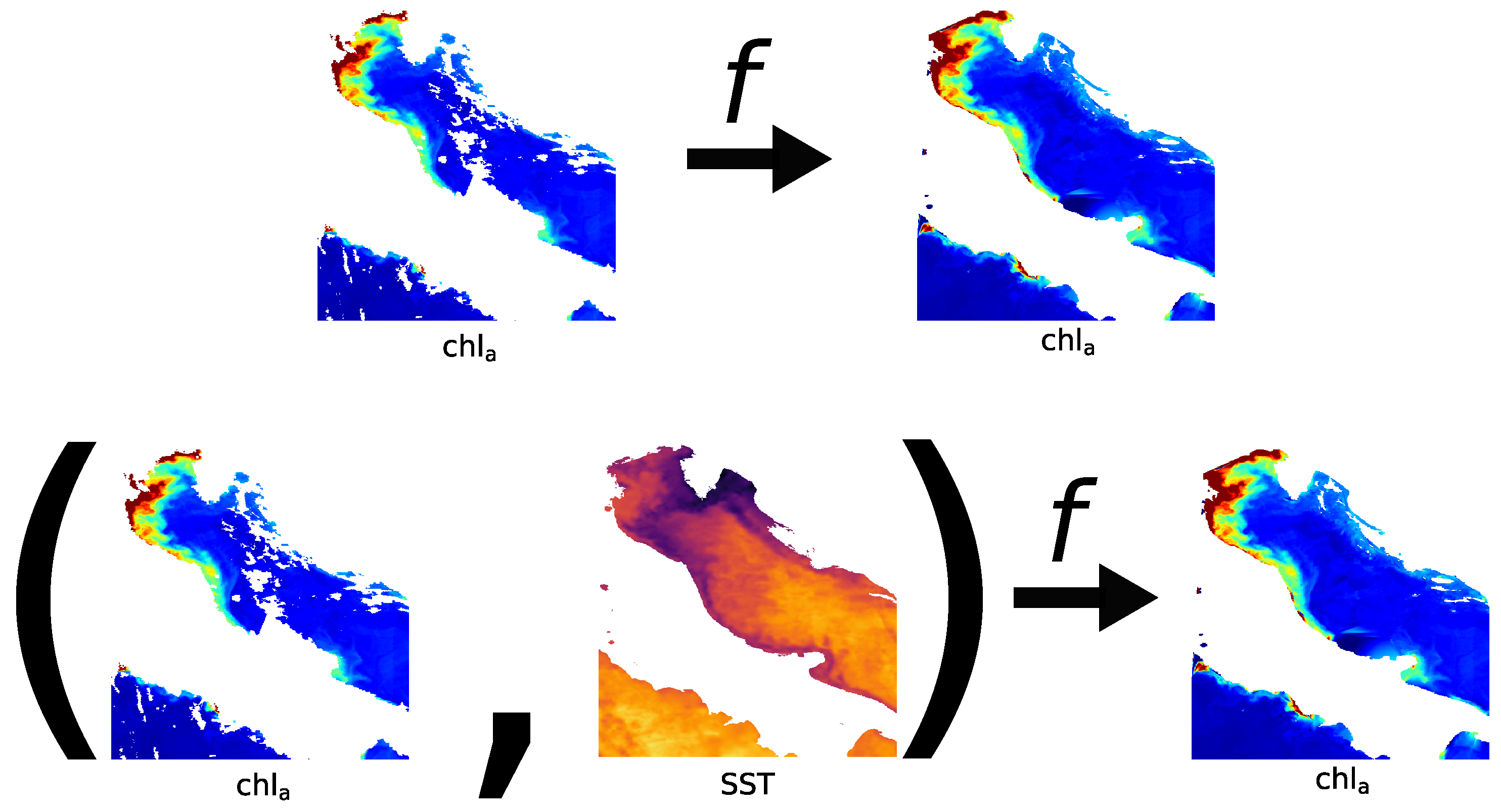
Figure 3.
Examples of unitemporal (top row) and multitemporal (bottom row) approaches being used for reconstruction. The targeted time-instance is . Both examples imply available data have been composited with reconstructed missing data to obtain complete data, .
Figure 3.
Examples of unitemporal (top row) and multitemporal (bottom row) approaches being used for reconstruction. The targeted time-instance is . Both examples imply available data have been composited with reconstructed missing data to obtain complete data, .
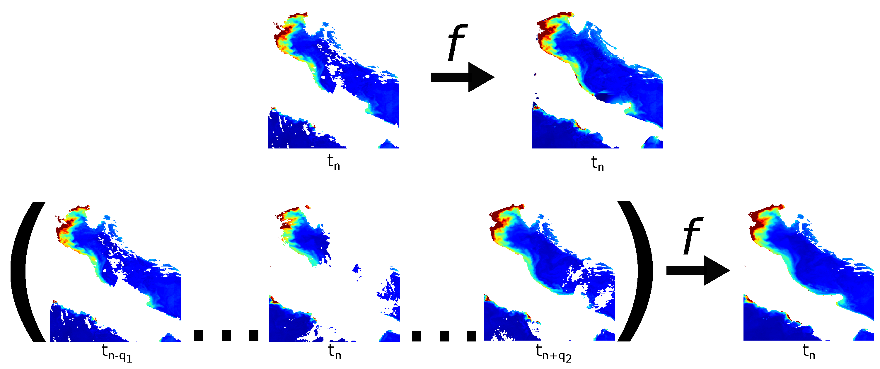
Figure 6.
A simple DT for sorting the numbers A, B and C, assuming no two are equal. Since the DT is well defined, every leaf corresponds to possible sorting order.
Figure 6.
A simple DT for sorting the numbers A, B and C, assuming no two are equal. Since the DT is well defined, every leaf corresponds to possible sorting order.
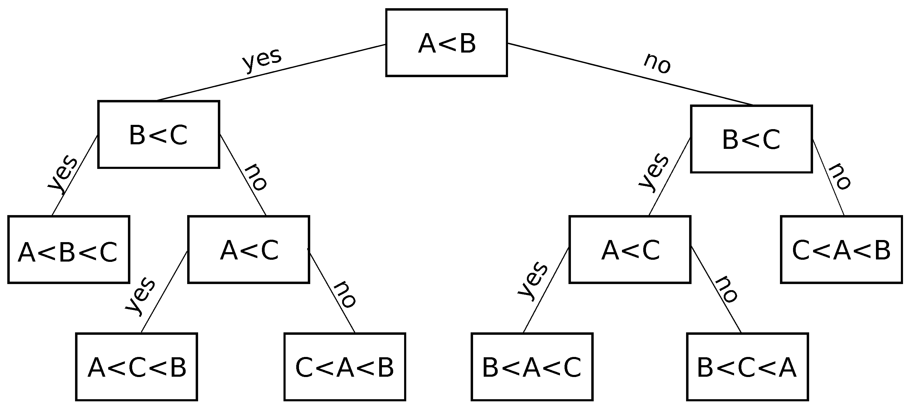
Figure 7.
Visualisation of the popularity of the methods. While (a) showcases the aforementioned trend in popularity, (b) displays the overall popularity of methods, with EOF-based methods being the most popular.
Figure 7.
Visualisation of the popularity of the methods. While (a) showcases the aforementioned trend in popularity, (b) displays the overall popularity of methods, with EOF-based methods being the most popular.
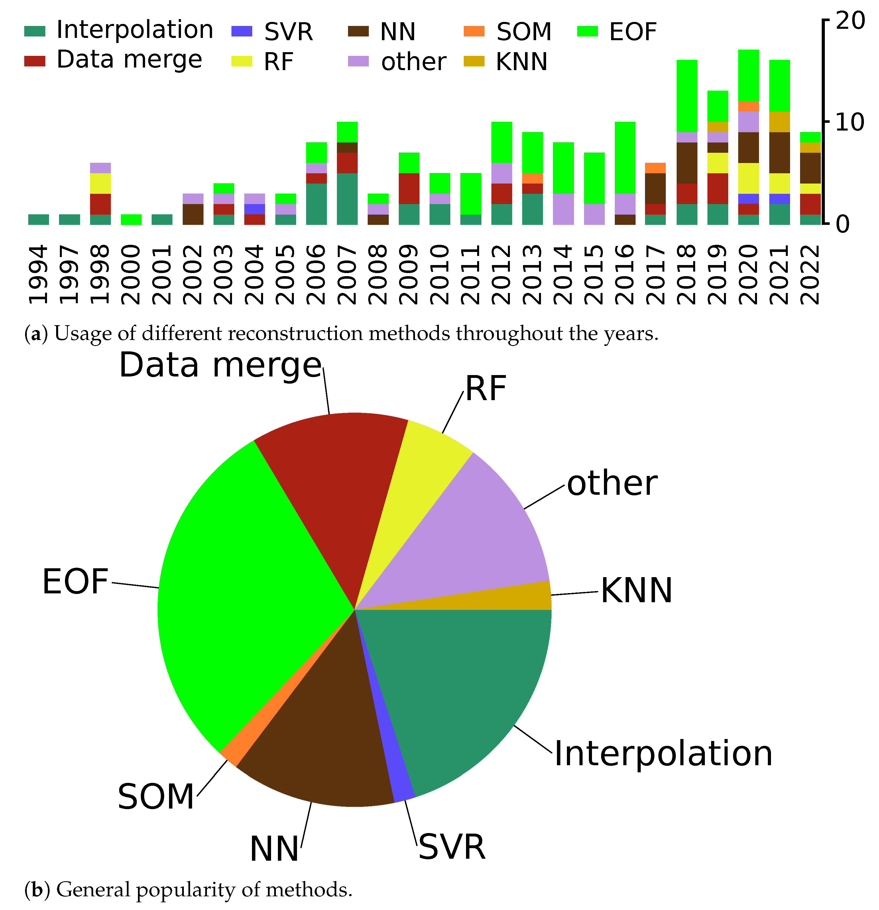
Table 1.
Reconstruction approaches sorted according to the novel variate-temporal categorisation system.
Table 1.
Reconstruction approaches sorted according to the novel variate-temporal categorisation system.
| Unitemporal | Multitemporal | |
|---|---|---|
| Univariate | [35,38,41,42,48,51,59,60,61,68, 74,75,76,79,80,84,97,98,99,105,108, 113,114,115,116,117,122,124,126,129,137,138,141,148, 152,153,156,158,163,192] | [30,31,32,34,37,39,40,43,44,45,47,50,51,52,54, 55,57,58,59,63,64,66,68,69,71,72,73,74,76,77,78,79, 81,82,83,85,86,87,91,93,100,101,104,105, 107,108,109,110,111,112,113,117,119,120,121,125,127,128,130,133, 135,139,140,142,143,144,147,148, 150,151,152,154,155,158,162,163,164,193,194,195,121] |
| Multivariate | [29,36,46,49,53,56,61,62,65,67,94,106, 118,123,131,132,136,145] | [29,64,67,70,88,89,90,92,93,95,96,102,146, 157,195] |
Table 2.
Surveyed articles cross-referenced against the target data and utilised reconstruction method.
Table 2.
Surveyed articles cross-referenced against the target data and utilised reconstruction method.
| SST | Other | ||
|---|---|---|---|
| EOF | [30,34,37,39,43,44,45, 50,51,52,58,59,63,66, 69,70,71,72,73,74,77,78,79,81,82,85, 87,88,89,90,91,92,93,95,133,135,148,157] | [43,44,52,55, 87,88,89,90,91,92,93, 95,105,107,119,120,125,127, 128,142,143,144,150,151, 162,191,193,194,195] | [29,30,31,33,40,45, 50,52,85,87,93,101, 102,104,130,148,195] |
| SVR | [74,84] | [56] | [84] |
| Interp. | [38,47,57,60,64,67,68, 73,76,83,86,132,157] | [47,54,108,109,110,111,112, 113,117,120,121,140,152,153, 154,162,191,193,194] | [54,83,86,99,100,158, 163,164] |
| KNN | [67,74] | n/a | [163,164] |
| RF | [62,67,74,75,157] | [56,106] | [163] |
| SOM | [64,157] | n/a | [96] |
| NN | [59,61,65,70,74,134, 137] | [49,56,94,105,106,115, 120,121,122,123,124,147,192] | [94,137,139] |
| Data merge | [35,46,51,68,79,131,148, 149] | [46,48,108,113,114, 117,152] | [41,42,97,98,148,149, 158] |
| other | [36,53,76,80,92,136,138, 155,156,157] | [92,116,118,126,138, 141,145,146,162,192] | [29,32,53,100,103,129, 136,138] |
Disclaimer/Publisher’s Note: The statements, opinions and data contained in all publications are solely those of the individual author(s) and contributor(s) and not of MDPI and/or the editor(s). MDPI and/or the editor(s) disclaim responsibility for any injury to people or property resulting from any ideas, methods, instructions or products referred to in the content. |
© 2023 by the authors. Licensee MDPI, Basel, Switzerland. This article is an open access article distributed under the terms and conditions of the Creative Commons Attribution (CC BY) license (https://creativecommons.org/licenses/by/4.0/).
Share and Cite
MDPI and ACS Style
Ćatipović, L.; Matić, F.; Kalinić, H. Reconstruction Methods in Oceanographic Satellite Data Observation—A Survey. J. Mar. Sci. Eng. 2023, 11, 340. https://doi.org/10.3390/jmse11020340
AMA Style
Ćatipović L, Matić F, Kalinić H. Reconstruction Methods in Oceanographic Satellite Data Observation—A Survey. Journal of Marine Science and Engineering. 2023; 11(2):340. https://doi.org/10.3390/jmse11020340
Chicago/Turabian StyleĆatipović, Leon, Frano Matić, and Hrvoje Kalinić. 2023. "Reconstruction Methods in Oceanographic Satellite Data Observation—A Survey" Journal of Marine Science and Engineering 11, no. 2: 340. https://doi.org/10.3390/jmse11020340
Note that from the first issue of 2016, this journal uses article numbers instead of page numbers. See further details here.