Extreme Heavy Rainfall Events at Mid-Latitudes as the Outcome of a Slow Quasi-Resonant Ocean—Atmosphere Interaction: 10 Case Studies

Abstract

Based on case studies, the development of low-pressure systems leading to extreme precipitation events reveals common characteristics. They highlight the co-evolution of sea surface temperature (SST) anomalies and the clustering of mesoscale convective systems in characteristic period ranges according to harmonic modes of the annual declination of the sun. This suggests a quasi-resonance of the heat exchanges of the ocean and the atmosphere during cyclogenesis. The formation of coherent extensive positive SST anomalies in characteristic period ranges, which reflects various interactions from baroclinic waves at mid-latitudes, i.e., Rossby waves especially present where the western boundary currents move away from the continents, may be a precursor of an extreme heavy rainfall event. Fed by warm and humid air coming from coherent SST anomalies, the convective cyclonic system strengthens concomitantly with the formation of cut-off lows, favoring blocks. However, the concentration in space and time of large-amplitude rainfall anomalies requires a relative stability of the atmospheric blocking circulation during the slow maturation processes. Intensification of extratropical cyclones is presumably the consequence of natural and anthropogenic warming, which strengthens the mechanisms leading to the clustering of mesoscale convective systems. The present study should help to refine the prediction of these extreme events while contributing to enrich our understanding of their presumed link with global warming.

1. Introduction

The baroclinic instability of the quasi-zonal westerly atmospheric flow is the main physical mechanism for the generation and development of mid-latitude cyclones. Being generated as a result of baroclinic instability of the atmosphere, cyclones further evolve under the influence of a number of factors, including but not limited to the interaction of the atmosphere and the sea surface (i.e., heat and moisture exchange) [1]. The latent heat is an important energy source of developing cyclonic eddies. An increase in sea surface temperature (SST) under global warming is accompanied by an intensification of the processes of water vapor “injection” into the atmosphere and an increase in the energy potential of cyclonic formations. The study of effects of the atmosphere and ocean interaction on the development and evolution of cyclones and associated precipitation zones and vice versa is of great scientific and practical interest.

Low-pressure systems forming at mid-latitudes are inducing more and more frequent extremely heavy precipitation events. Several studies show that they increase with global warming [2,3,4,5,6,7] almost everywhere in the world [8,9]. These events are particularly devastating because they can occur in areas known to be non-flood-prone, at unusual times of the year. For these reasons, such events are very difficult to predict. Indeed, they powerfully impact the polar jet stream, forming cut-off lows when a closed upper-level low wraps around the low-pressure system so that the jet stream becomes displaced from the basic westerly current and moves independently of that current. As an example, in July 2021, severe flooding occurred across Europe, hitting Germany the hardest where many people lost their lives [10]. These events are surprising by the speed with which mesoscale convective systems are formed, causing very heavy large-scale rainfall on an almost-stationary convergence zone. Synoptic low-pressure systems promote cut-off lows [11], favoring blocks, which enables the relatively slow co-evolution of the interactions between the atmosphere and the ocean.

The difficulty in predicting the extent of such events as well as their possible link with anthropogenic warming supports active research given their significant social and economic impact [12]. From case studies selected from the exceptional amount of precipitation observed during a day, the purpose of the present paper is to highlight and clarify the conditions of formation of Extreme Rainfall Events (EREs) at mid-latitudes. This is achieved from the representation of the amplitude and phase of SST and precipitation anomalies by using the joint wavelet analysis of SST and rainfall data in different period ranges. This investigative work is made possible thanks to the high-quality data of precipitation that combines information from the Global Precipitation Measurement (GPM) satellite constellation.

2. Materials and Methods

2.1. Data

Daily gridded data (1/4° × 1/4°) of the Sea Level Anomaly (SLA) are provided by the National Oceanic and Atmospheric Administration (NOAA) [13].

Daily (1/4° × 1/4°) SST data are provided by the NOAA [14,15,16,17]. The data are averaged on grids (1° × 1°) to obtain a resolution adapted to the needs of the present study.

Version 06 of daily (0.2° × 0.2°) data of precipitation (2000 to present) combines information from the GPM (Global Precipitation Measurement) satellite constellation to estimate precipitation over the majority of the Earth’s surface [18].

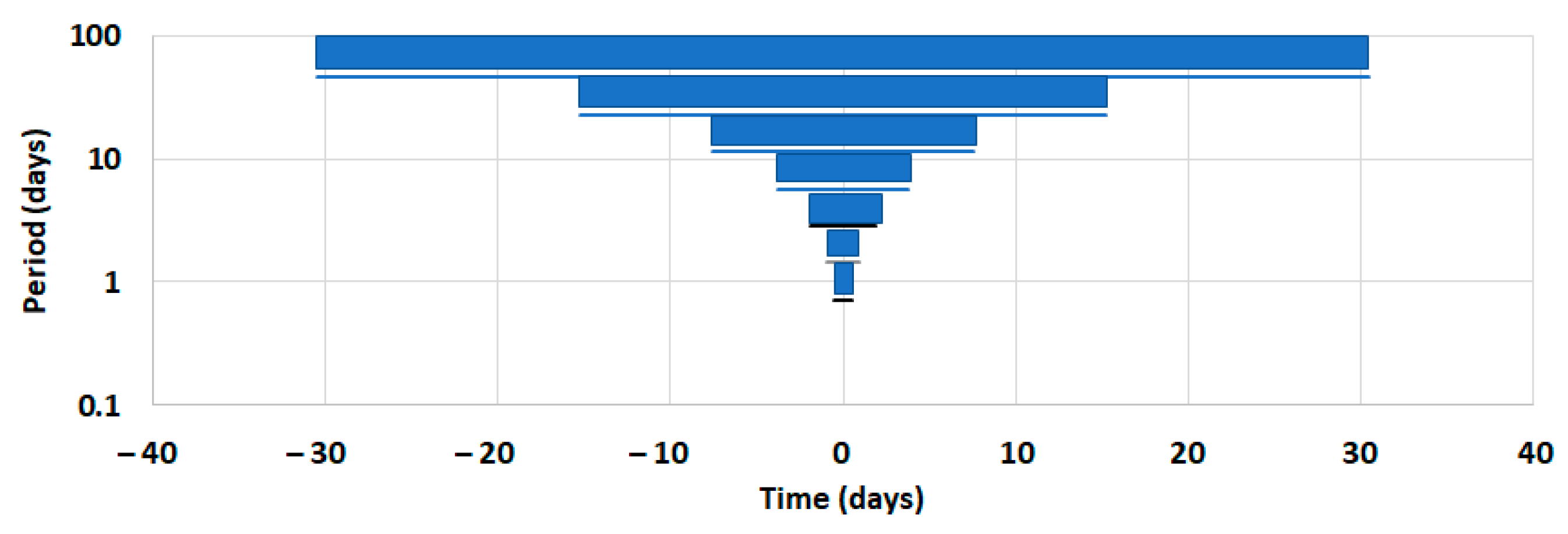
2.2. Decomposition of SST and Preciptation Data in Period Ranges

The method that is followed here is exposed in [19] for the study of marine heat waves, i.e., sudden positive SST anomalies resulting from sea–atmosphere interactions and subtropical cyclones. The decomposition of the spatialized SST and precipitation data into period ranges, averaged over time intervals whose duration equals the average widths of the bands, makes it possible to highlight the co-evolution of precipitation and SST anomalies. Taking the date of occurrence of the ERE as a temporal reference, for each period range, the precipitation and SST data are each represented on two paired maps. The first represents the amplitude of the anomalies independently of the date of occurrence of the ridge within the time interval, and the second represents the phase, i.e., the time lag of the ridge relative to the date of occurrence of the ERE.

This decomposition according to the period ranges is performed by using the Morlet wavelet analysis of the data [20]. The period ranges are represented in

Table 1. Contiguous bandwidths used in wavelet analysis.

Harmonic	Mean Period (days)	Lower Limit (Days)	Upper Limit (Days)
1/6	60.9	45.7	91.3
1/12	30.4	22.8	45.7
1/24	15.2	11.4	22.8
1/48	7.6	5.7	11.4
1/96	3.8	2.9	5.7
1/192	1.9	1.43	2.9
1/384	0.95	0.71	1.43

and in Figure 1. For periods shorter than 2.9 days, the evolution of the cyclonic systems could not be approached using the same method, which would require better temporal resolution data, and a spatial resolution of a few kilometers, which is not the purpose of the present paper.

The choice of bands is based on the different harmonics of the annual period, i.e., the declination period of the sun. This choice results from the interactions between the ocean and the atmosphere that have a major role in the genesis of extreme precipitation events. The positive SST anomalies that intervene in the various interactions result primarily from baroclinic waves at mid-latitudes, i.e., Rossby waves especially present around the oceanic gyres, and coastal Kelvin waves [21,22]. However, as these baroclinic waves are resonantly forced by variations in ocean temperature as well as by seasonal westerly winds, their amplitude oscillates according to various harmonic modes. This property is evidenced by the Caldirola–Kanai (CK) Oscillator, which is a fundamental model of dissipative coupled oscillator systems. This very general formulation applies to multi-frequency baroclinic ocean waves [19]. The oscillation of such coupled oscillators in harmonic modes ensures their durability and stability.

The different harmonic modes are observed by carrying out a frequency analysis of the sea level anomalies (SLAs) where the western boundary currents move away from the continents, as is the case for the Gulf Stream at 39.875° N, 65.125° W (Figure 2). As shown in Figure 2, the Fourier Transform of SLA and SST display a main peak centered on the annual period and several harmonics. The main harmonics of SLA are centered on the 1/3-year period, then the following harmonics are deduced from it by successively dividing the periods by 2. The main period of SST is annual, reflecting the declination of the sun, accompanied by one harmonic centered on the 1/2-year period.

Figure 2d shows that the variables SLA and SST are significantly coherent within broad bands, which reflects a causal relationship between SLA and SST. Rossby waves being approximately nondispersive, they propagate west along the eastward propagating wind-driven current of the North Atlantic gyre in which they are embedded. The resultant velocity of Rossby waves faces east because their phase velocity is lower than the velocity of the wind-driven current. The apparent wavelength of Rossby waves is proportional to the period so that they form a mosaic of convergent or divergent cells depending on whether the geostrophic currents U and V associated with them converge or diverge within these cells, which extend longitudinally over an apparent half-wavelength [19].

The uplift of the thermocline that occurs in divergent cells enhances evaporation from the ocean surface, while the lowering of the thermocline that occurs in convergent cells causes them to behave as heat sinks. When phase homogenization of a positive SST anomaly occurs locally, it tends to expand as a result of subsequent evaporation and condensation processes, which favors the uniformization of the motion of the thermocline owing to the exchange of sensible and latent heat between warm and cold cells.

This phenomenon helps to explain the formation of marine heat waves as have occurred in the northwestern Pacific Ocean [19]: the SST anomaly has been translated over extensive areas of the northwestern Pacific Ocean, including the Yellow Sea, the entire Sea of Japan, and part of the Sea of Okhotsk, as did SLA. In the case of extratropical cyclones, this mechanism resulting in the coherence of the movement of the thermocline on a large scale can be invoked where the western boundary currents move away from the continents, and well beyond.

If one ignores the effect of direct radiation on SST, the latter should, therefore, be inversely correlated with SLA. Actually, as shown in Figure 2e, the combined effect of geostrophic currents and radiation on the ocean surface induces a phase shift between the SLA and the SST, which depends on the period range. The SST can be ahead of the SLA as it occurs for the 1/24 and 1/4 harmonic modes, or, on the contrary, it lags as it occurs for the 1/12 harmonic mode and the fundamental mode.

2.3. Morlet Wavelet Analysis

The amplitude of SST and rainfall anomalies is expressed from the square root of their Morlet wavelet power, scale-averaged over a period range [20]. The time lag between the date of occurrence of the ridge of the anomalies and the brief ERE is deduced from the cross-wavelet power of the variables, and the rainfall depth at a location representative of the ERE, which is used as the time reference, scale-averaged over a period range [19].

In Table 1 and Figure 1, the first three bands reflect the harmonic modes observed for SLA. The next four are presumed modes extended to short periods for an exhaustive description of the variables. The variable sampling interval, which is one day, does not allow the observed periods to be further reduced. Bandwidths are deduced from the mean period T of harmonics. Lower and upper limits are 0.75 × T and 1.5 × T, respectively, so the bands are contiguous as the periods are halved from one harmonic to another.

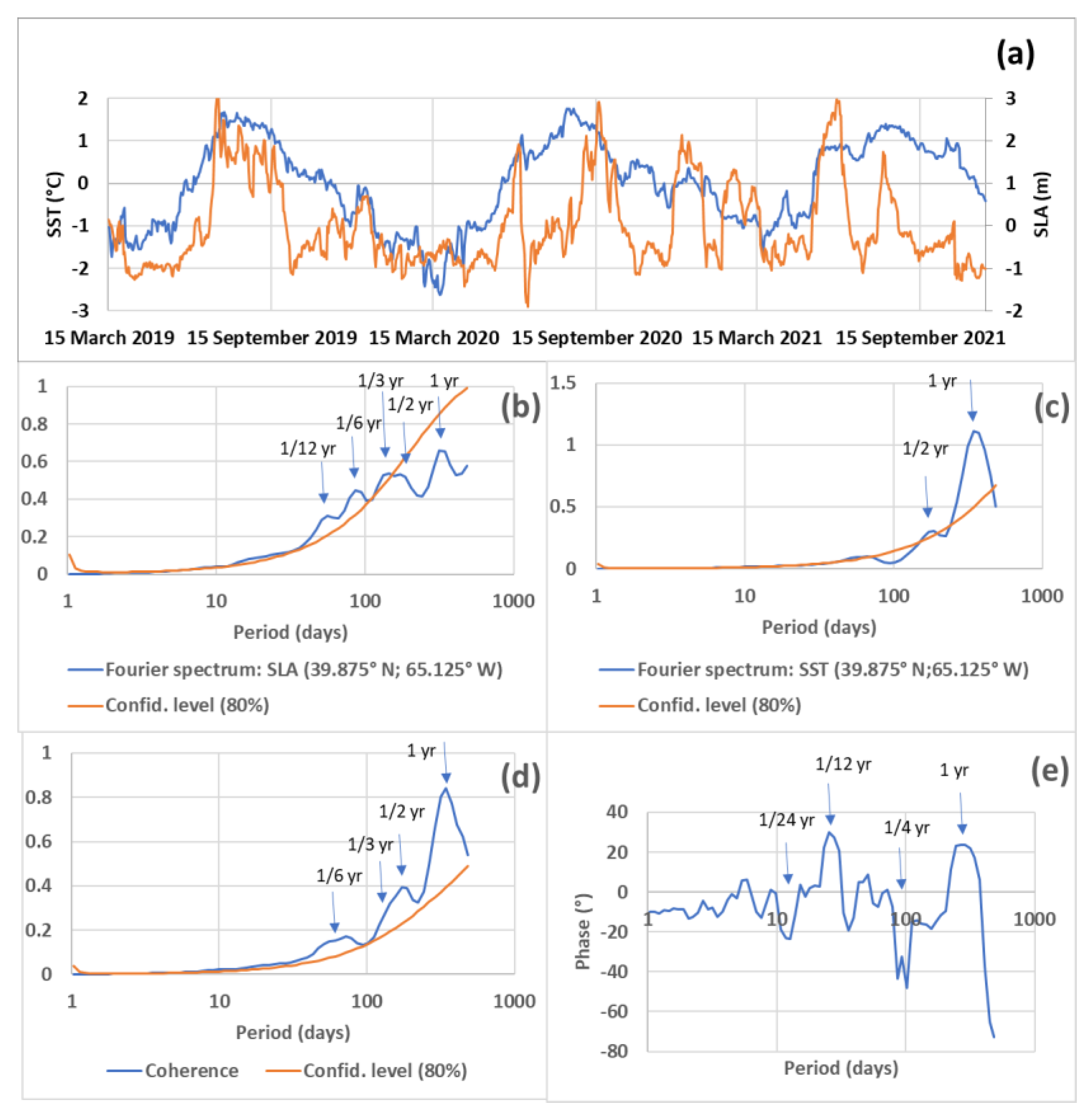
2.4. Coherence and Phase of Rainfall and SST Anomalies According to Harmonic Modes

The purpose of this section is to prove the hypothesis that atmospheric phenomena and SST anomalies evolve in a concerted manner during the genesis of extra-tropical cyclones. For that, the coherence of precipitation at a given location and SST anomalies presumably involved in cyclogenesis is estimated from a long series of precipitation in a region of southeastern United States and SST in various regions off the southeastern and eastern coasts of North America. The joint analysis of these different temporal data in a characteristic period range is discussed wherever the coherence is greater than a 95% confidence level [20].

2.4.1. Exceptional Rainfall Episodes in Characteristic Period Ranges

For the purposes of clarity, the choice of the regions represented in Figure 3 is justified by the fact that the coherence of the precipitation and SST data is best resolved there in a narrow period range, which is the 22.8–45.7-day band according to the 1/12-year harmonic (Figure 1). It is in this band that the coherence best reflects the link between the two variables, i.e., precipitation and SST, which is evidenced by the height of the peaks compared to their level of confidence. The coherence in the 22.8–45.7-day band of the precipitation depth, and the SST anomalies averaged over the four regions exhibited in Figure 3 are represented in Figure 4. Precipitation depth is averaged over a (86° W, 82° W) × (33° N, 37° N) region (Figure 4a,b).

Seven precipitation episodes whose amplitude is averaged in the 22.8–45.7-day band (Figure 1) have a 3-year return period (Figure 4b). This band represents 45% of the total precipitation amount. The coherence in the 22.8–45.7-day band of precipitation height and SST anomalies in each of the four selected regions off the coast of southeastern North America (Figure 3) is represented in Figure 4c. It clearly shows that the coherence of the precipitation and the SST anomaly in region 1 makes it possible to discriminate the episodes whose return period is 3 years (Figure 4d). Indeed, the episodes whose coherence with the SST anomaly of region 1 is greater than 0.15, whose level of confidence is close to 95%, highlight each of the 7 exceptional events. In all cases, another region is associated with the exceptional event, identifiable from the coherence of the precipitation and the SST anomaly in the corresponding region. This is usually region 2 except for episode 4. Although less significant, regions 3 and 4 are involved in almost all episodes, except for episodes 4 and 2, respectively. The coherences relating to the various regions are in phase almost everywhere except for regions 2, 3, and 7 for which the coherences relating to region 1 lag behind the others.

Episodes 8, 9, 10, and 11 are also discriminated, although they have a return period of less than 3 years, which means that the stated conditions are necessary for the formation of exceptional rainfall episodes but are not sufficient. In fact, the 11 selected rainfall episodes all occur in winter and spring and there is nothing to distinguish between them. It can be deduced that the mechanisms leading to the concentration of precipitation in the 22.8–45.7-year band do not only depend on the SST, but also on the evolution of the atmospheric blocking circulation during the rainfall episode.

The choice of the band according to the 1/12 harmonic is not fortuitous, because, as seen later (Extreme Precipitation in February 2020, in Kentucky, USA), clustering of mesoscale lows and harmonization of the thermocline depth both occur in that band.

2.4.2. Exceptional Rainfall Amount for One Day

The phenomenon of quasi-resonance, which occurs in the band of the 1/12 harmonic when (1) clustering of mesoscale lows in a synoptic convective system occurs; (2) SST anomalies develop coherently on a large scale and nearly in phase with the ERE, which supposes harmonization of the thermocline depth; (3) the cut-off low has a very slow movement over the confined region, can result in the exceptional concentration of rainfall amount both in space and in time. This is what occurs for episodes 2, 3, 6, and 7 during which an exceptional precipitation amount is observed during less than one day. Two events whose return period is nearly 10 years are observed in episodes 3 and 6 on 12 October 2008 and 6 February 2020, with the rainfall depth during a day being, respectively, 113 and 111 mm. Five events with a rainfall depth greater than 90 mm have a return period close to 4.2 years. In addition to the two previous events, three events have a rainfall depth of about 90 mm, occurring on 6 February 2004, 31 March 2005, and 25 March 2021. The rainfall depth during a day is, respectively, 95, 91 and 91 mm. The latter two occur during episodes 2 and 7, while the former occurs outside of any characterized time period. In this case, the coherence, which is 0.123, is poorly significant. It is a sudden event similar to how there is one every winter, with the low-pressure system being favored by the warm sea of the Gulf of Mexico, but here, the height of precipitation is relatively high as, within this context, it rarely exceeds 80 mm in one day.

Thus, this case study justifies the method that aims to characterize, from the coherence of SST anomalies and rainfall depth resulting from exceptional events, the co-evolution of the two variables. However, this supposes the relative stability of the atmospheric blocking circulation. As already stated, it is a sine qua non condition for the extratropical cyclone to induce a concentration of rain in space and time whose amplitude is exceptional.

This case study is chosen for its relative simplicity because clustering of mesoscale lows and harmonization of the thermocline depth both occur in the same period scale. The case studies show that this property is not always true; the co-evolution of the cyclonic system and SST anomalies can occur in two adjacent bands while being concomitant (in phase). In this case, the coherence of the two variables should have been established in a wider band associating the two harmonics concerned as a result of the overlapping of the actual bands. However, the best way to prove a causal relationship between the two variables stems from their spatialization, as is performed for the different case studies.

3. Results

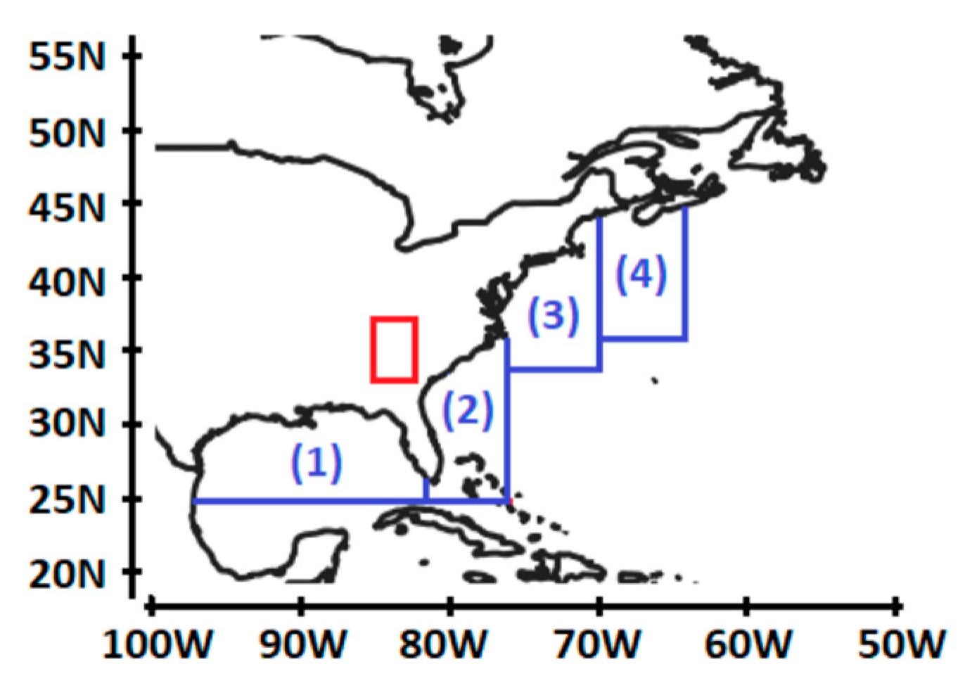
3.1. SST Anomalies That Fuel the Heavy Rainfall Are Developing along an Eastern Boundary Current

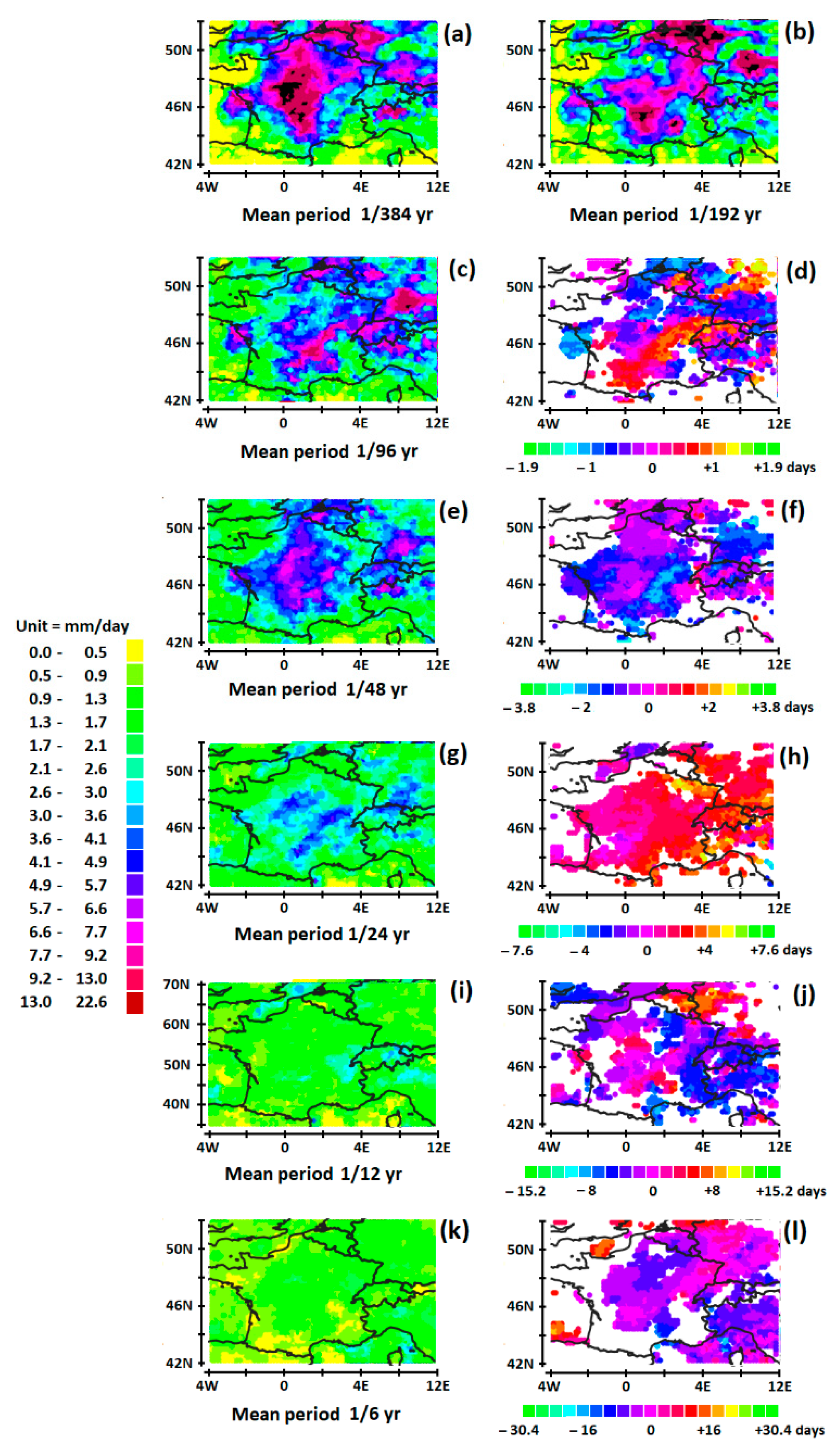
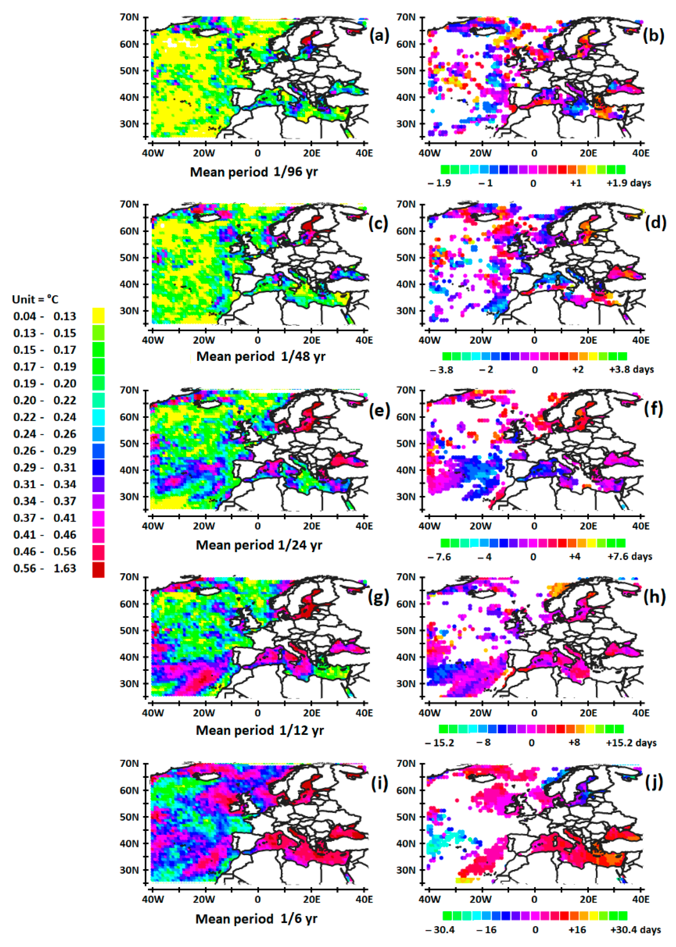
3.1.1. A Demonstrative Case Study: The Extreme Precipitation Events That Occurred in Western and Northern Europe in June 2016

The heavy rains began on May 26th when a large cut-off low spurred the development of several slow-moving low-pressure disturbances [7]. Fueled by warm and humid air from the south, this caused clusters of heavy thunderstorms (Mesoscale Convective System) in Germany and very heavy large-scale rainfall combined with showers on an almost-stationary convergence zone over France. The 3-day precipitation in the Seine basin was very rare in April–June, with a return time of roughly one in hundreds of years. In Germany, Gundelsheim (also Baden-Württemberg) reported 122 mm between 6 am on May 29th and 6 am the next day.

Evolution of Rainfall Anomalies in Characteristic Period Ranges

The amplitude and phase of both precipitation depth and SST anomalies in the seven period ranges are shown in Figure 5 and Figure 6, respectively. From Figure 5, the peak of rainfall anomalies increases when the period decreases. This highlights the acceleration of the convergence of the cyclonic system as the period decreases.

The 1/384 and 1/192 harmonics of precipitation reach 22.6 mm/day over 0.2° × 0.2° gridded data in both cases. As the temporal sampling interval corresponds, for each of the two harmonics, to approximately 1 and 2 days, this means that the precipitation depth overreaches 40 mm within two days where the anomalies overlap, i.e., in Belgium, western Germany, the center of France, and in the south of the French Massif Central. Rainfall anomalies are at high latitudes, between 46° N and 51° N, and they are far from each other, between 0° and 9° E in longitude.

The fragmentation of the phase, which increases as the period decreases, reflects a time lag in the evolution of the fragmented low-pressure systems whatever the time scale. However, the 1/24 harmonic of precipitation is an exception to this rule. The phase homogenizes remarkably, which suggests clustering of mesoscale lows in a synoptic convective system over a large part of Europe. A question arises. Can the particular behavior of the low-pressure systems in the 11.4 to 22.8-day band be observed during the evolution of all extratropical cyclones?

Co-Evolution of SST and Rainfall Anomalies in Characteristic Period Ranges

In Figure 6g,h, the behavior of the 1/12 harmonic of SST anomalies of the seas and oceans involved in the genesis and the fueling of the extratropical cyclone here again stands out. The phase of the 1/12 harmonic of SST anomalies, which are two main branches stretching southwest–northeast, is uniform, and nearly concomitant with the ERE, while the phase of SST anomalies is fragmented and/or out of phase in the other period ranges. SST anomalies greater than 0.46 °C in the period range of 22.8–45.7 days occur along the Canary Current off Morocco and western Sahara in the North Atlantic Ocean up to a longitude close to 40° W, on the western part of the Mediterranean Sea, on the western part of the Baltic Sea, and on the North Sea. The Atlantic SST anomalies are located far south of the center of the depression concerned by the heavy rains, under latitude 37° N.

However, the co-evolution of the low-pressure systems and the SST anomalies do not occur in the same period range, namely 11.4–22.8 and 22.8–45.7 days. This seems to show that, in the particular context of Western Europe with its different seas far from the core of the extratropical cyclone, the homogenization of the SST phases occurs more slowly than the clustering of the low-pressure systems in the core of the depression. However, these peripheral SST anomalies, which are in phase with the ERE, contribute to fueling the extratropical cyclone. Its diameter reaches more than 1000 km, the center of France, the south of the Massif Central, Belgium, and northern Germany being, respectively, under the influence of the Atlantic Ocean, the Mediterranean Sea, the Baltic Sea, and the North Sea off the coast of Denmark.

3.1.2. Extreme Precipitation in June 2005, in Alberta, Canada

One of Canada’s most devastating floods occurred in southern Alberta in June 2005. Three major storms spread out over the month of June drenched the area [23]. Cumulative rainfall varied, ranging from between 50 and 100 mm falling in the Edmonton area, to more than 400 mm falling in and around High River.

Evolution of 1/384 and 1/192 Harmonics of Precipitation

Only the figures corresponding to the 1/384 and 1/192 harmonics of precipitation and the 1/12 harmonic of precipitation and SST anomalies are represented in Figure 7. In Figure 7a,b, the 1/384 and 1/192 harmonics of the precipitation depth highlight anomalies in the South of Alberta and Saskatchewan, Canada, which means deep continental penetration. Rainfall anomalies form two branches stretching southwest–northeast between latitudes 49° N and 57° N. The sum of the main precipitation anomalies in the southernmost branch overreaches 100 mm in two days.

Co-Evolution of SST and Rainfall Anomalies in Characteristic Period Ranges

From Figure 7c,d, clustering of rainfall anomalies occurs in the two branches, where the 1/12 harmonic of the precipitation is almost in phase with the ERE. The SST anomaly greater than 0.40 °C, made up of two branches, develops along the California Current, between latitudes 30° N and 40° N (Figure 7e,f). The two branches are strongly out of phase. The southernmost branch is almost 8 days ahead of the occurrence of the ERE. The northernmost branch, the only one supplying the extratropical cyclone, is a few days behind the occurrence of the ERE, which means that the ERE occurs a little before the anomaly reaches its peak.

As in the case of the extreme rainfall that occurred in western and northern Europe, this one occurs in June, fueled by a positive SST anomaly that forms along the eastern boundary current. Fueled by warm and humid air from the SST anomaly to the south, the cyclonic system strengthens above the land, which has not yet warmed up at the end of spring.

3.2. SST Anomalies That Fuel the Heavy Rainfall Are Developing along a Western Boundary Current

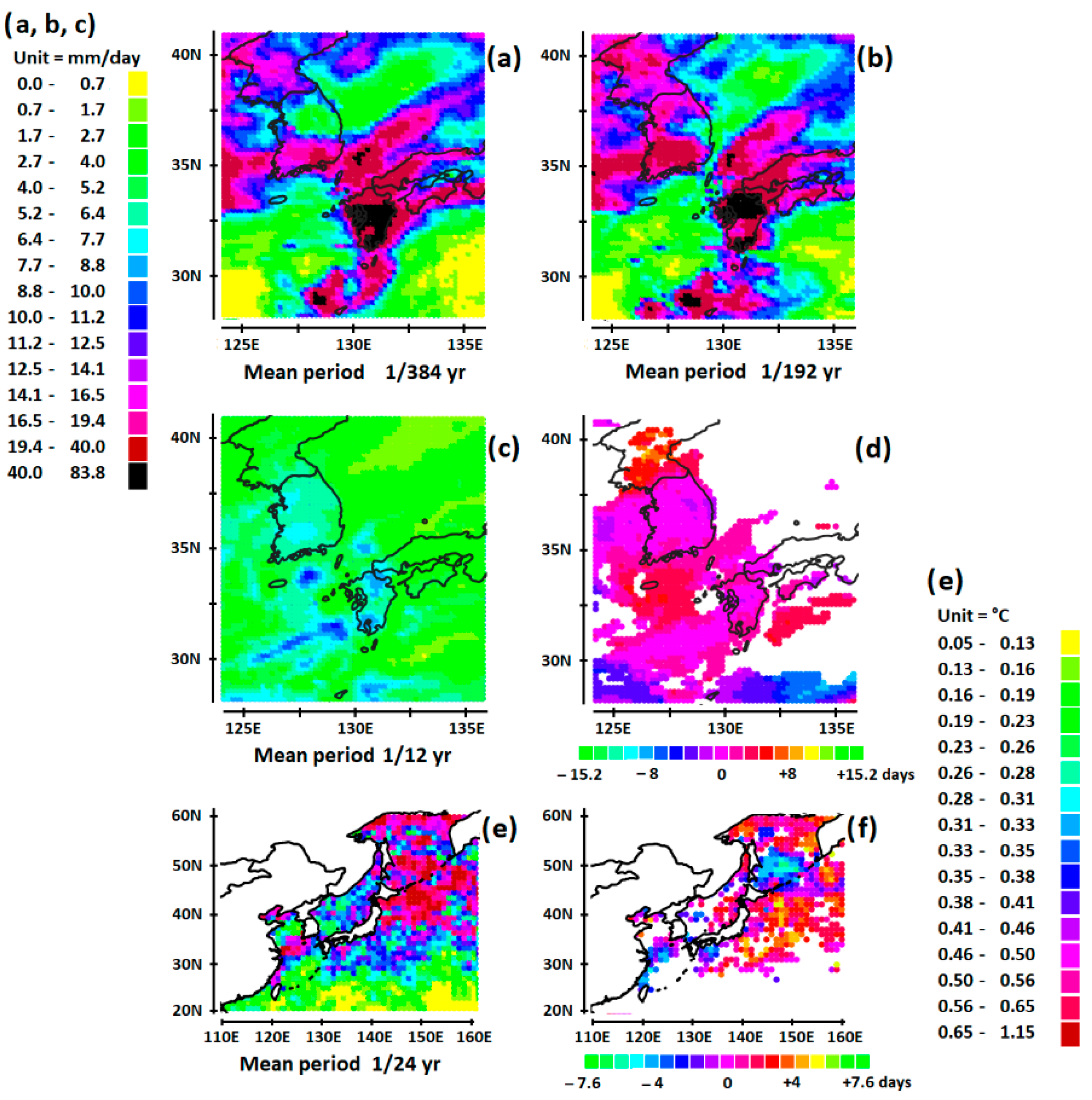
3.2.1. Extreme Precipitation in July 2012, in Japan

In July 2012, heavy rains fell on the Japanese main island of Kyushu, causing floods and landslides, especially in northern regions [24]. Accumulated precipitation reached 1130 mm in the center of Kyushu.

Evolution of 1/384 and 1/192 Harmonics of Precipitation

Rainfall anomalies nearly in phase with the ERE occur in South Korea and the south of Japan, forming two main branches oriented southwest–northeast. The main anomaly, at the south of Japan, is located between 31 and 33° N. The precipitation depth overreaches 150 mm in two days (Figure 8a,b).

Co-Evolution of SST and Rainfall Anomalies in Characteristic Period Ranges

Clustering of mesoscale lows occurs in tune with the 1/12 harmonic (Figure 8c,d), involving the two branches of rainfall anomalies. On the other hand, harmonization of the thermocline depth occurs in tune with the 1/24 harmonic (Figure 8e,f). An SST anomaly greater than 0.56 °C, a few days behind the ERE, is located in the Sea of Japan and in the Pacific Ocean along the Kuroshio (Figure 8e,f). Thus, the ERE occurs while the peak of the SST anomaly has not quite peaked yet.

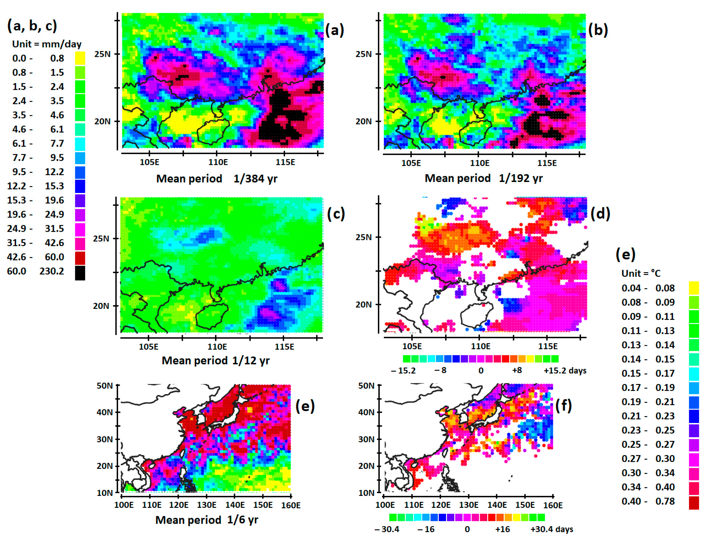
3.2.2. Extreme Precipitation in June 2020, China

In 2020, large parts of eastern Asia experienced their wettest summer for almost 60 years [25]. Studies highlighted the stationarity of the monsoon front, which was controlled by the upper-level flow pattern, with the jet stream and the west Pacific high pressure playing a leading role [26].

Evolution of 1/384 and 1/192 Harmonics of Precipitation

The main rainfall anomaly occurs in the China Sea between 18° N and 22° N, reaching 230 mm in one day and overreaching 400 mm in two days (Figure 9a,b). An anomaly close to the main anomaly occurs at 113° E, 22.5° N in southern Guangdong, and another at 107.2° E, 23° N in southern Guangxi, both greater than 60 mm in one day.

Co-Evolution of SST and Rainfall Anomalies in Characteristic Period Ranges

SST anomalies nearly in phase with the ERE are included between 0.40 and 0.78 °C in the South and East China Sea and the Pacific Ocean along the Kuroshio, off the southeastern coast of China, up to longitude 142° E (Figure 9e,f). They are concomitant with the 1/6 harmonic while clustering of mesoscale lows occurs in tune with the 1/12 harmonic (Figure 9c,d).

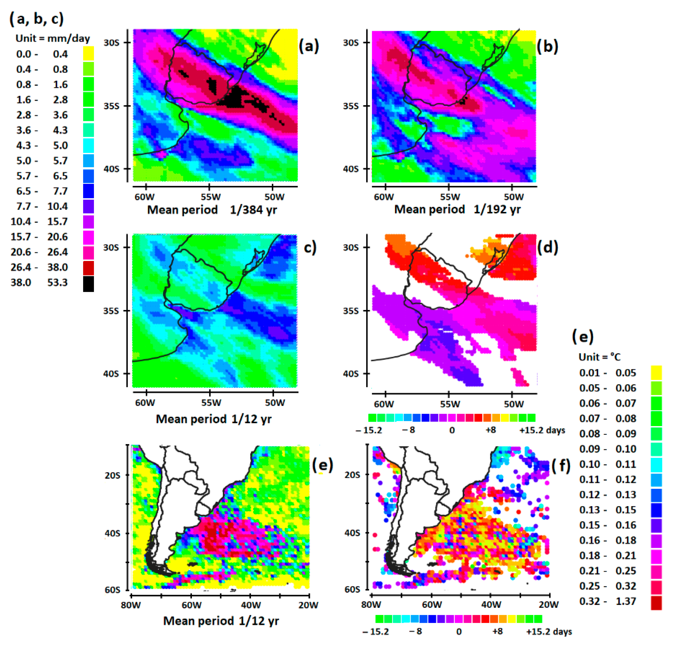
3.2.3. Extreme Precipitation in August 2015, Argentina

Several locations in the northern Buenos Aires Province suffered flash floods in August 2015, caused by record rain, with accumulated precipitation reaching between 250 and 300 mm in a southeast–northwest-oriented strip crossing Uruguay and the Argentinian provinces Entre Rios and Santa Fe [27].

Evolution of 1/384 and 1/192 Harmonics of Precipitation

The main rainfall anomaly is a band oriented southeast–northwest, crossing Uruguay and the two Argentinian provinces Entre Rios and Santa Fe (Figure 10a,b). The anomaly, which is located between 38 and 30° S, reaches up to 53.3 mm in one day.

Co-Evolution of SST and Rainfall Anomalies in Characteristic Period Ranges

SST anomalies between 0.32 and 1.37 °C are located along the warm Brazil current of the South Atlantic gyre, after it collides with the northerly flowing cold-water Malvinas Current, a few days behind the ERE (Figure 10e,f). Homogenization of the thermocline depth occurs in tune with the 1/12 harmonic, as well as clustering of mesoscale lows (Figure 10c,d).

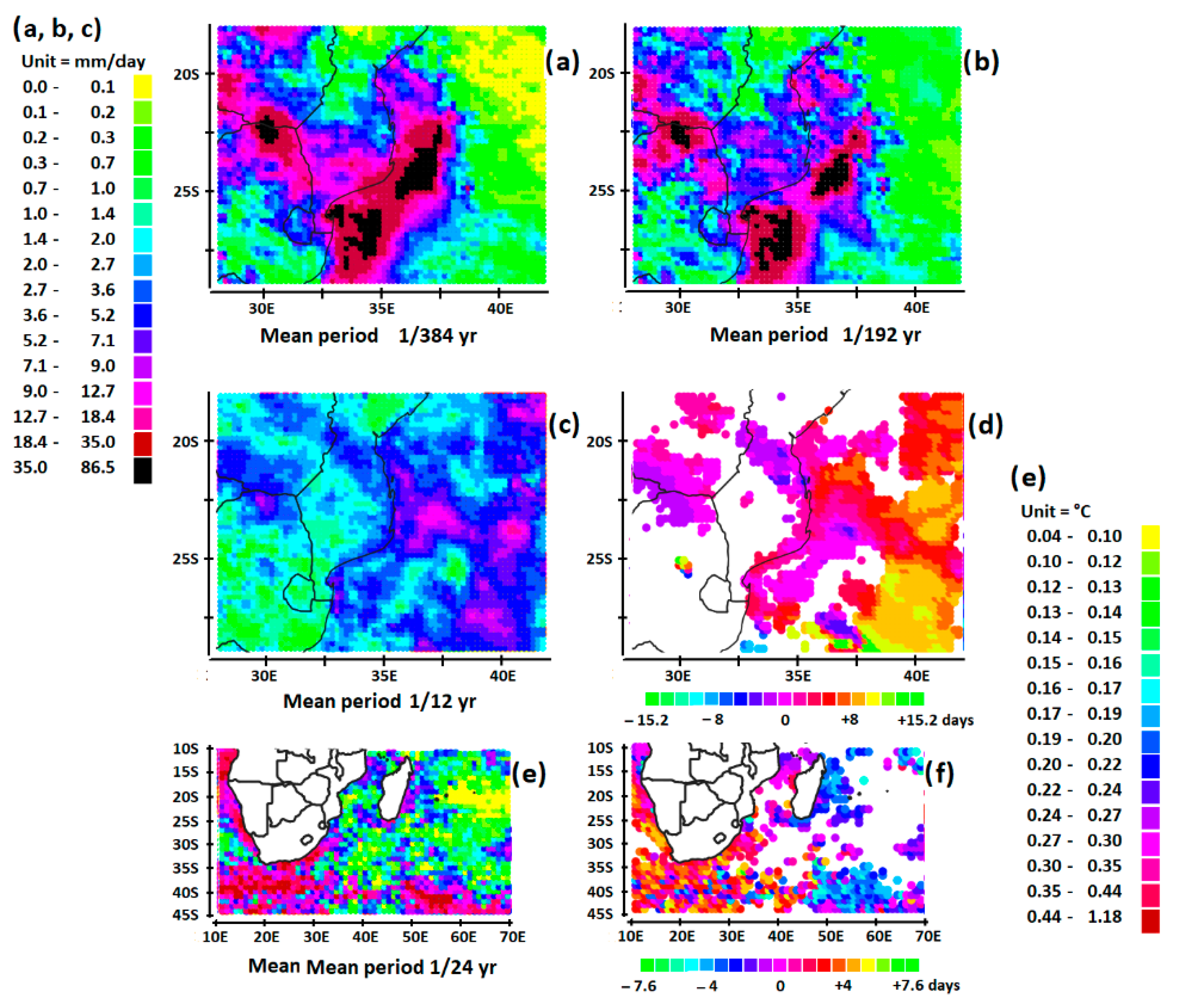
3.2.4. Extreme Precipitation in February 2007, Mozambique

Between December 2006 and February 2007, heavy rains across northern and central Mozambique, together with severe rainfall in neighboring countries, led to flooding along the Zambezi River Basin in Tete, Manica, Sofala, and Zambezia provinces [28]. Cyclone Favio slammed into Central Mozambique on 22 February 2007, pounding the country with winds over 200 km per hour and drenching rains. After coming ashore in southern Mozambique, the storm tracked northwest over the country. It quickly lost power as it moved inland, but its rains impacted river systems in Central Mozambique.

Evolution of 1/384 and 1/192 Harmonics of Precipitation

Three main rainfall anomalies are located between 20° S and 29° S. They reach between 35 and 86.5 mm in one day and nearly double in two days in the Indian Ocean off the Maputo region at the southernmost tip of Mozambique, and further north off the Inhambane region (Figure 11a,b). The third anomaly is on the border of South Africa and Zimbabwe. The southernmost tip of Mozambique is impacted close to the coast.

Co-Evolution of SST and Rainfall Anomalies in Characteristic Period Ranges

Clustering of mesoscale lows occurs in tune with the 1/12 harmonic while the phase shows a slow motion of the core of the low-pressure system oriented northwest–southeast (Figure 11c,d). SST anomalies between 0.44 and 1.18 °C, which are a few days late on the ERE, develop along the Agulhas current as it flows south of the African continent before retroflecting when it meets the Benguela current flowing up along the southwestern coast of Africa (Figure 11e,f). Homogenization of the thermocline depth occurs in tune with the 1/24 harmonic (Figure 11c,d).

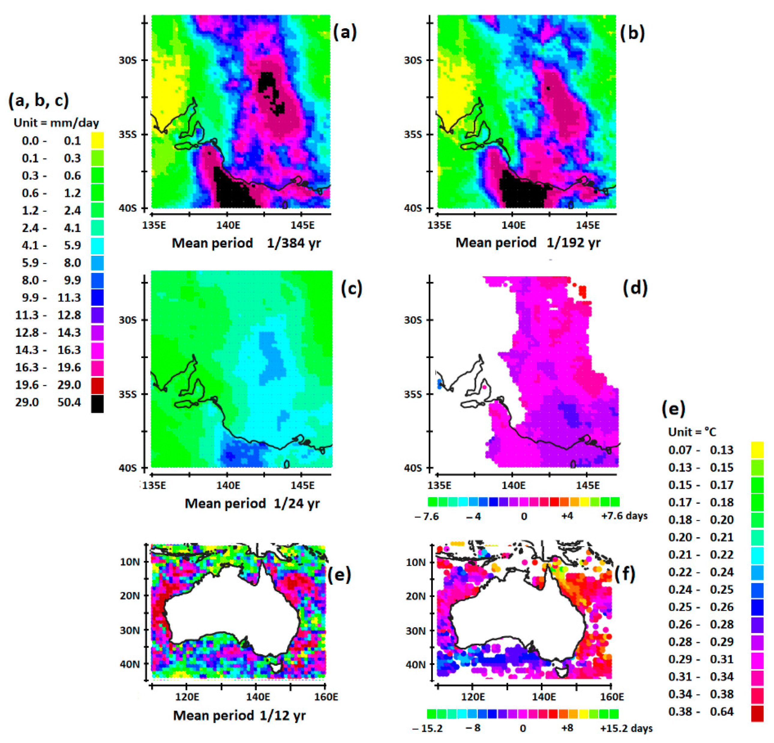
3.2.5. Extreme Precipitation in January 2011, in Victoria, Australia

Total rainfall across Victoria is the largest in history. Some locations have not seen these totals as records began 130 years ago. Kyneton and Maryborough in central Victoria have recorded their highest ever summer rainfall in the past 24 h [29]. Up to 150 mm of rain fell in some parts of Victoria in the last 24 h. A lot of locations in the west have actually exceeded their whole summer average in just five days. High-intensity rainfall between 12 and 14 January 2011 caused major flooding across much of the western and central parts of the Australian state of Victoria.

Evolution of 1/384 and 1/192 Harmonics of Precipitation

Two rainfall anomalies are located between 30° S and 40° S. The most southerly is in the Indian Ocean off Victoria while the second, more northerly, is in the western part of Victoria and New South Wales and the eastern part of South Australia (Figure 12a,b). The southernmost anomaly reaches 50 mm in one day and nearly double in two days.

Co-Evolution of SST and Rainfall Anomalies in Characteristic Period Ranges

Clustering of mesoscale lows occurs in tune with the 1/24 harmonic (Figure 12c,d), while the extratropical cyclone is moving slowly south–north. Two SST anomalies between 0.38 and 0.64 °C are located in the Pacific Ocean off the coasts of southeastern and northeastern Australia (Figure 12e,f). The SST anomaly off the coast of southeast Australia occurs along the western boundary current, i.e., the Eastern Australian Current Extension, and the SST anomaly off the coast of northeast Australia occurs along the South Equatorial Current. Both SST anomalies are a few days behind the ERE.

3.2.6. Extreme Precipitation in February 2020, in Kentucky, USA

Major flooding inundated Southeast Kentucky in 6–7 February 2020, i.e., in winter when the temperature difference is maximum between the warm waters of the Gulf of Mexico and the mainland. Beginning on February 3rd, heavy rainfall events continued through February 7th. Rain amounts of 100–150 mm fell across much of southeastern Kentucky over this period [30].

Evolution of 1/384 and 1/192 Harmonics of Precipitation

The rainfall anomaly located between 30° N and 39° N reaches between 50 and 59.1 mm in one day, exceeding 100 mm in two days. It elongates in a southwest–northeast direction over Alabama, Georgia, east of Tennessee, west of north and South Carolina, and south of Kentucky (Figure 13a,b).

Co-Evolution of SST and Rainfall Anomalies in Characteristic Period Ranges

Two SST anomalies between 0.62 and 1.29 °C are located in the northern part of the Gulf of Mexico and along the Gulf Stream, up to 65° W (Figure 13e,f). They are concomitant with the 1/12 harmonic, with clustering of mesoscale lows as well (Figure 13c,d). The peak of the SST anomalies is 4 days behind the occurrence of the ERE, which means that the convergence process of the low-pressure system accelerated during the growing phase of the SST anomaly.

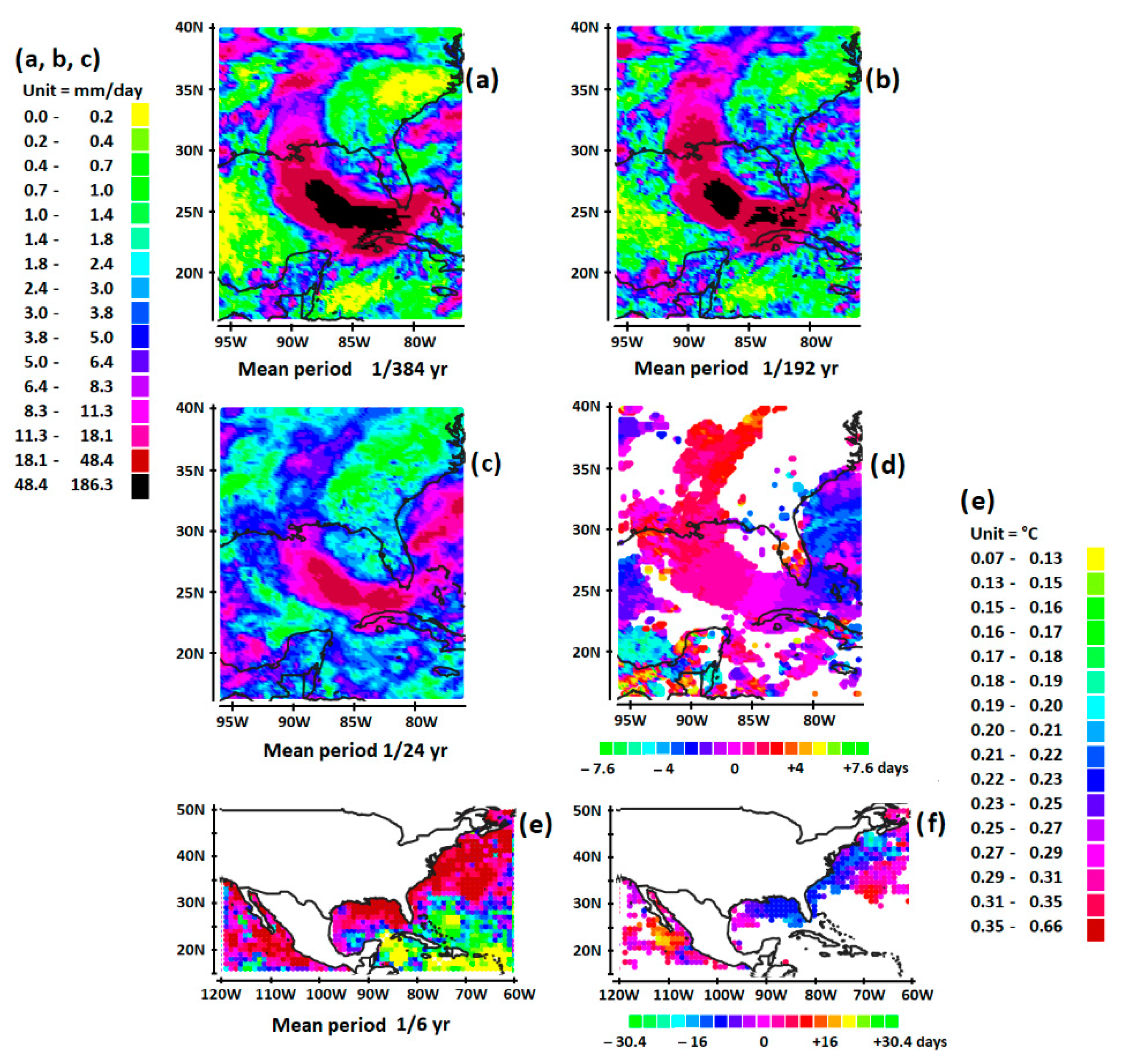
3.2.7. Extreme Precipitation in August 2005, in Louisiana, USA

The storm that would later become Hurricane Katrina surfaced on 23 August 2005, as a tropical depression over the Bahamas, 560 km east of Miami [31]. Over the next two days, the low-pressure system strengthened, becoming Tropical Storm Katrina, and making landfall between Miami and Fort Lauderdale, Florida, as a Category 1 hurricane, with winds in the range of 120 to 150 km/h. Sustained winds swept across the Florida peninsula and 130 mm of rainfall was reported in some areas. The storm quickly intensified as it reached the warm waters of the Gulf of Mexico.

On August 27, Katrina upgraded to a Category 3 hurricane, with winds exceeding 185 km/h. Then, Katrina became one of the most powerful Atlantic storms on record, with winds exceeding 275 km/h. On the morning of August 29, the storm made landfall as a Category 4 hurricane in Plaquemines Parish, Louisiana, 70 km southeast of New Orleans. It continued on a northeasterly course, crossing the Mississippi Strait and making a second landfall later in the morning near the mouth of the Pearl River.

Here, it was no longer an extratropical cyclone but a tropical cyclone that originated in the Gulf of Mexico, then migrated north. However, this migration could only be accomplished in the presence of SST anomalies feeding the cyclone once it left the Gulf of Mexico at mid-latitudes.

Evolution of 1/384 and 1/192 Harmonics of Precipitation

A rainfall anomaly extends on an arcuate band starting west from the southeast end of the Gulf of Mexico, then north in two days to Louisiana, Mississippi, and Alabama, ending in a northeast direction to Arkansas and Tennessee (Figure 14a–d). At the center, the anomaly is between 48.4 and 186.3 mm in one day, overreaching 300 mm in two days.

Co-Evolution of SST and Rainfall Anomalies in Characteristic Period Ranges

Homogenization of the thermocline depth occurs in tune with the 1/6 harmonic (Figure 14e,f). The SST anomalies between 0.35 and 0.66 °C extend off the southeastern coasts of North America on both sides of Florida, both in the Gulf of Mexico and the Atlantic Ocean along the Gulf Stream. They anticipate the formation of the cyclone by a few days: the peak of the SST anomaly occurs 8 days before the ERE, whereas the formation of the tropical cyclone off the eastern coast of Florida, Georgia, and South Carolina occurs 4 days before the ERE (Figure 14c,d).

The SST anomaly off the southeastern coast of USA favors the formation of the tropical cyclone. It behaves as a guide in the southward migration of the depression before its track curves west off the Bahamas, then north, supplied by the SST anomaly in the Gulf of Mexico.

3.3. Extreme Precipitation in October–November 2011, in Mediterranean Countries

3.3.1. A Tropical-Like Storm

The tropical-like storm of November 2011 started over the period 4–6 November 2011, when an extratropical system slowly transformed into a subtropical low over the warm waters of the Mediterranean Sea. As the storm moved slowly westward, it caused flooding in Spain and the Balearic Islands, then slowly organized and convection began to increase [32,33].

On 7 November 2011, the subtropical area of low pressure was located in the Gulf of Lions, as the storm organized itself into a subtropical disturbance. Later that day, the subtropical disturbance transformed and strengthened, into a tropical-like depression off the coast of France. Late on November 7, the storm was upgraded to tropical-like storm status as it strengthened significantly. On 8 November 2011, the storm continued to strengthen as it came closer to France. At peak intensity, the storm had a minimum low pressure of 991 hPa. On November 9, however, the storm made landfall in south-eastern France, near Hyeres, where it dissipated completely shortly thereafter.

Overall, the tropical-like storm caused severe flooding, in parts of Spain, Italy, and France. From 6 to 8 November 2011, the storm produced a total of 600 mm of rain in about 72 h over southwestern Europe.

Particularly devastating, the accurate prediction of Mediterranean tropical-like cyclones is an important challenge for numerical weather prediction models. A study of the sensitivity of an intense tropical cyclone, which formed south of Sicily on 7 November 2014, has been carried out, based on microphysical patterns involving the formation of cumulus clouds as well as the surface layer [32].

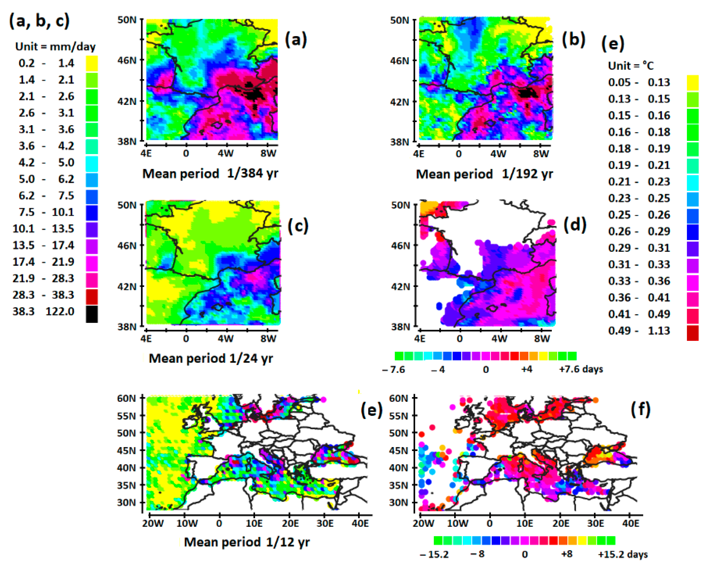
3.3.2. Extreme Precipitation in France, 4 November 2011

Evolution of 1/384 and 1/192 Harmonics of Precipitation

Close to the latitude 42° N, the rainfall anomaly between 38.3 and 122 mm in one day, more than 200 mm in two days, extends over the Mediterranean Sea off the southern coast of France. It impacts the southeastern region of France close to the Mediterranean coast (Figure 15a,b).

Co-Evolution of SST and Rainfall Anomalies in Characteristic Period Ranges

Clustering of mesoscale lows occurs in tune with the 1/24 harmonic, resulting in a compact cyclonic system in the Mediterranean Sea off the southeastern coast of France (Figure 15c,d). SST anomalies greater than 0.4 °C are located in the central part of the Mediterranean Sea, the Adriatic Sea, but also, in the north, the Baltic Sea as well as the North Sea South of the Scandinavian countries (Figure 15e,f). They are concomitant with the 1/12 harmonic. On the other hand, the Atlantic Ocean is absolutely not involved in the formation of the low-pressure system. The peak of the SST anomalies is 4 days behind the occurrence of the ERE over France.

4. Discussion

The development of coherent SST anomalies fueling synoptic-scale extratropical cyclones reflects a phenomenon of quasi-resonance that occurs in specific period ranges according to harmonic modes of ocean–atmosphere interactions. In the case of the mid-latitude migration of tropical cyclones, studied here from a single case study, namely the cyclone Katrina, the quasi-resonance results in the formation and the migration of the tropical cyclone.

The synoptic cyclonic systems result from the clustering of mesoscale convective systems highlighted from the homogenization of the phase of rainfall anomalies concomitantly with the ERE in characteristic period ranges according to 1/24 or 1/12 harmonic modes of the declination of the sun. Ocean–atmosphere interactions result in the harmonization of the thermocline depth over large scales (homogenization of the phase of SST anomalies concomitantly with the ERE) in characteristic period ranges according to 1/24, 1/12, or 1/6 harmonic modes. Fed by warm and humid air coming from coherent SST anomalies, the convective cyclonic system strengthens concomitantly with the formation of cut-off lows, favoring blocks. These synoptic low-pressure systems can lead to the concentration in space and time of large-amplitude rainfall anomalies, which requires a relative stability of the atmospheric blocking circulation.

4.1. SST Anomalies Develop along an Eastern Boundary Current

When SST anomalies develop along an eastern boundary current approaching the continent by flowing toward lower latitudes, they occur at lower latitudes than the center of the subtropical cyclone to establish a difference in sufficient temperature with mainland. The two cases studied occur in spring. These events migrate more and more toward high latitudes as global warming progresses.

4.2. SST Anomalies Develop along a Western Boundary Current

When fed by SST anomalies developing along western boundary currents, subtropical cyclones become particularly intense when SST anomalies extend into lower latitudes beyond the western boundary current. This is what occurs for the devastating Kentucky floods when the SST anomaly extends both in the northern part of the Gulf of Mexico and along the Gulf Stream off Georgia and North and South Carolina. This is also what favored the migration of tropical hurricane Katrina to the north, affecting Louisiana. This also occurs in southeastern China when SST anomalies develop both in the South and East China Sea and the Pacific Ocean along the Kuroshio, off the south-eastern coast of China. In Japan, SST anomalies develop both in the Sea of Japan and in the Pacific Ocean along the Kuroshio, off the southeastern coast of Japan. In southeast Australia, SST anomalies occur both along the Eastern Australian Current Extension and along the South Equatorial Current. As for Mozambique, SST anomalies develop both along the South Equatorial Current of the Indian Ocean and along the Agulhas current as it flows south of the African continent. Concerning Argentina, an SST anomaly occurs along the warm Brazil current, after it collides with the northerly flowing cold-water Malvinas Current. Here, it is the extension of the SST anomaly along the Brazil Current after it moves away from the continent that matters in the intensity of the cyclone.

These extratropical cyclones usually occur in early boreal/austral summer when the temperature difference between the SST anomalies along the western boundary current and the mainland is large. There are two exceptions, however, the Kentucky and Argentina floods that occurred in February and August, respectively. For Kentucky, the ERE occurred in winter when the temperature difference is maximum between the warm waters of the Gulf of Mexico and the mainland. Concerning Argentina, most flash floods occur during the austral summer. From this point of view, the case study chosen is not fully representative of what is generally observed.

4.3. SST Anomalies Develop in the Mediterranean Sea

When fed by an SST anomaly developing in the Mediterranean Sea, tropical-like storms become particularly devastating when coherent SST anomalies occur in the Adriatic Sea, or even in the Baltic Sea, and the North Sea off the Scandinavian coast. They usually occur at the end of summer when the Mediterranean Sea is warmest.

4.4. Potential Link with Global Warming

The analysis of the different stages leading to extratropical low-pressure systems makes it possible to address an essential problem, which relates to the presumed impact of anthropogenic forcing. The ubiquity of the increase in the frequency as well as the intensity of EREs suggests an evolution in the mechanisms favoring the development at the synoptic scale of cyclonic flows. Indeed, an increase in the temperature of the surface of the oceans favors evaporative processes, which lowers the dew point and favors the formation of fronts as well as the transfer of sensible and latent heat between the atmosphere and the ocean, hence positive feedback. This hypothesis is corroborated by the fact that EREs occur more and more frequently in places deemed to be not subject to flooding. This is especially true for extreme precipitation events that result from SST anomalies developing along an eastern boundary current.

The concomitance of the phenomena at the origin of the ERE blurs the slow phenomena of maturation that occur in the ranges of periods centered on 1/6, 1/12, and 1/24 years. Monitoring these processes could help predict the occurrence of devastating meteorological phenomena.

5. Conclusions

The selected case studies differ depending on whether the SST anomalies that fuel the ERE are developing along an eastern boundary current (2 cases), along a western boundary current (7 cases), or in the Mediterranean Sea and the semi-enclosed seas of Europe (1 case). However, they have one common characteristic. The occurrence of extreme heavy rainfall events is the outcome of a slow process of ocean–atmosphere interaction of a quasi-resonant nature, in characteristic period ranges. These sudden and violent events always occur if fueled by warm, moist air resulting from SST anomalies, contributing to the formation of synoptic low-pressure systems. They require the co-evolution of SST anomalies and clustering of mesoscale lows in a synoptic convective system, with the ridge of SST and mesoscale precipitation anomalies being nearly concomitant with the sudden extremely heavy precipitation event. To lead to a rainfall event of extreme amplitude, the slow process of maturation of the cyclonic system has to induce the early formation of an upper-level cut-off low involving a stable atmospheric blocking circulation during the maturation phase.

Intensification of extratropical cyclones as well as the increase in their frequency is presumably the consequence of anthropogenic warming, which strengthens the mechanisms leading to the coalescence of mesoscale lows. The present study should help to refine the prediction of these extreme events—the formation of coherent extensive SST anomalies in characteristic period ranges may be a precursor of an extreme heavy rainfall event—while contributing to enrich our understanding of their presumed link with global warming.

References

1. Cotton, W.R.; Bryan, G.H.; van den Heever, S.C. Storm and Cloud Dynamics, International Geophysics; Elsevier: Amsterdam, The Netherlands, 2011; eBook; ISBN 9780080916651. [Google Scholar]
2. Myhre, G.; Alterskjær, K.; Stjern, C.W.; Hodnebrog, Ø.; Marelle, L.; Samset, B.H.; Sillmann, J.; Schaller, N.; Fischer, E.; Schulz, M.; et al. Frequency of extreme precipitation increases extensively with event rareness under global warming. Sci. Rep. 2019, 9, 16063. [Google Scholar] [CrossRef] [PubMed]
3. Sillmann, J.; Kharin, V.V.; Zwiers, F.W.; Zhang, X.; Bronaugh, D. Climate extremes indices in the CMIP5 multimodel ensemble: Part 2. Future climate projections. J. Geophys. Res. Atmos. 2013, 118, 2473–2493. [Google Scholar] [CrossRef]
4. Giorgi, F.; Coppola, E.; Raffaele, F. A consistent picture of the hydroclimatic response to global warming from multiple indices: Models and observations. J. Geophys. Res. Atmos. 2014, 119, 11695–11708. [Google Scholar] [CrossRef]
5. Lehmann, J.; Coumou, D.; Frieler, K. Increased record-breaking precipitation events under global warming. Clim. Change 2015, 132, 501–515. [Google Scholar] [CrossRef]
6. Fischer, E.M.; Knutti, R. Detection of spatially aggregated changes in temperature and precipitation extremes. Geophys. Res. Lett. 2014, 41, 547–554. [Google Scholar] [CrossRef]
7. van Oldenborgh, G.J.; Philip, S.; Aalbers, E.; Vautard, R.; Otto, F.E.L.; Haustein, K.; Habets, F.; Singh, R.; Cullen, H. Rapid attribution of the May/June 2016 flood-inducing precipitation in France and Germany to climate change. Hydrol. Earth Syst. Sci. 2016. [Google Scholar] [CrossRef]
8. Dong, S.; Sun, Y.; Li, C.; Zhang, X.; Min, S.-K.; Kim, Y.-H. Attribution of Extreme Precipitation with Updated Observations and CMIP6 Simulations. J. Clim. 2021, 34, 871–881. [Google Scholar] [CrossRef]
9. Sun, Q.; Zhang, X.; Zwiers, F.; Westra, S.; Alexander, L.V. A Global, Continental, and Regional Analysis of Changes in Extreme Precipitation. J. Clim. 2021, 34, 243–258. [Google Scholar] [CrossRef]
10. The July 2021 Floods in Germany and the Climate Crisis—A Statement by Members of Scientists for Future. Available online: https://info-de.scientists4future.org/the-july-2021-floods-in-germany-and-the-climate-crisis/ (accessed on 2 January 2023).
11. Ferreira, R. Cut-Off Lows and Extreme Precipitation in Eastern Spain: Current and Future Climate. Atmosphere 2021, 12, 835. [Google Scholar] [CrossRef]
12. Messori, G.; Bevacqua, E.; Caballero, R.; Coumou, D.; de Luca, P.; Faranda, D.; Kornhuber, K.; Martius, O.; Pons, F.; Raymond, C.; et al. Compound climate events and extremes in the mid-latitudes: Dynamics, simulation and statistical characterization. Bull. Am. Meteorol. Soc. 2021, 102, E774–E781. [Google Scholar] [CrossRef]
13. Sea Level Anomaly and Geostrophic Currents, Multi-Mission, Global, Optimal Interpolation, Gridded, Provided by the National Oceanic and Atmospheric Administration (NOAA). Available online: https://coastwatch.noaa.gov/pub/socd/lsa/rads/sla/daily/nrt/ (accessed on 19 November 2021).
14. Daily Sea Surface Temperature Is Provided by NOAA. Available online: https://www.ncei.noaa.gov/data/sea-surface-temperature-optimum-interpolation/v2.1/access/avhrr/ (accessed on 8 January 2022).
15. Reynolds, R.W.; Smith, T.M.; Liu, C.; Chelton, D.B.; Casey, K.S.; Schlax, M.G. Daily High-Resolution-Blended Analyses for Sea Surface Temperature. J. Clim. 2007, 20, 5473–5496. [Google Scholar] [CrossRef]
16. Banzon, V.; Smith, T.M.; Chin, T.M.; Liu, C.; Hankins, W. A long-term record of blended satellite and in situ sea-surface temperature for climate monitoring, modeling and environmental studies. Earth Syst. Sci. Data 2016, 8, 165–176. [Google Scholar] [CrossRef]
17. Huang, B.; Liu, C.; Banzon, V.; Freeman, E.; Graham, G.; Hankins, B.; Smith, T.; Zhang, H.M. Improvements of the Daily Optimum Interpolation Sea Surface Temperature (DOISST) Version v2.1. J. Clim. 2021, 34, 2923–2939. [Google Scholar] [CrossRef]
18. Temperature and Precipitation Gridded Data for Global and Regional Domains Derived from In-Situ and Satellite Observations, Provided by Copernicus. Available online: https://cds.climate.copernicus.eu/cdsapp#!/dataset/insitu-gridded-observations-global-and-regional?tab=formhttps://climate.copernicus.eu/esotc/2020/precipitations (accessed on 2 January 2023).
19. Pinault, J.-L. Morlet Cross-Wavelet Analysis of Climatic State Variables Expressed as a Function of Latitude, Longitude, and Time: New Light on Extreme Events. Math. Comput. Appl. 2022, 27, 50. [Google Scholar] [CrossRef]
20. Torrence, C.; Compo, G.P. A Practical Guide to Wavelet Analysis. Bull. Am. Meteorol. Soc. 1998, 79, 61–78. [Google Scholar] [CrossRef]
21. Pinault, J.-L. Regions Subject to Rainfall Oscillation in the 5–10 Year Band. Climate 2018, 6, 2. [Google Scholar] [CrossRef]
22. Pinault, J.-L. Global warming and rainfall oscillation in the 5–10 yr band in Western Europe and Eastern North America. Clim. Chang. 2012, 114, 621–650. [Google Scholar] [CrossRef]
23. Flooding in Alberta in 2005—An Overview. Available online: https://www.alberta.ca/release.cfm?xID=199938B24A678-B403-7562-2D1B4A3C14E15A79 (accessed on 11 November 2022).
24. Haeseler, S. Heavy Rains on Kyushu/Japan in July 2012. Available online: https://www.dwd.de/EN/ourservices/specialevents/precipitation/20120801_Kyushu_en.pdf?__blob=publicationFile&v=3 (accessed on 11 November 2022).
25. Extreme Rainfall in East Asia—Summer 2020, Met Office. Available online: https://www.metoffice.gov.uk/research/approach/collaboration/newton/insights/china---summer-2020-flooding (accessed on 11 November 2022).
26. Clark, R.T.; Dong, X.; Ho, C.-H.; Sun, J.; Yuan, H.; Takemi, T. Special Issue on Summer 2020: Record Rainfall in Asia—Mechanisms, Predictability and Impacts. Adv. Atmos. Sci. 2021, 38, 12. [Google Scholar] [CrossRef]
27. Argentina Flooding Kills Three, Leads to Thousands Evacuating Homes, ABC News. 12 August 2015. Available online: https://www.abc.net.au/news/2015-08-12/argentina-flooding-sparks-evacuation-of-thousands/6692118 (accessed on 11 November 2022).
28. Cyclone Favio Floods Mozambique, National Aeronautics and Space Administration (NASA). Available online: https://earthobservatory.nasa.gov/images/18053/cyclone-favio-floods-mozambique (accessed on 11 November 2022).
29. Hundreds Evacuated as Floods Threaten Victoria, ABC News, 14 January 2011. Available online: https://www.abc.net.au/news/2011-01-14/hundreds-evacuated-as-floods-threaten-victoria/1905122 (accessed on 11 November 2022).
30. Major Flooding Inundates Southeast Kentucky Followed by Light Snow from 6–7 February 2020, National Oceanic and Atmospheric Administration (NOAA). Available online: https://www.weather.gov/jkl/20200206_floodsnow (accessed on 11 November 2022).
31. Hurricane Katrina, Britannica. Available online: https://www.britannica.com/event/Hurricane-Katrina (accessed on 11 November 2022).
32. Pytharoulis, I.; Kartsios, S.; Tegoulias, I.; Feidas, H.; Miglietta, M.M.; Matsangouras, I.; Karacostas, T. Sensitivity of a Mediterranean Tropical-Like Cyclone to Physical Parameterizations. Atmosphere 2018, 9, 436. [Google Scholar] [CrossRef] [Green Version]
33. Kerkmann, J.; Bachmeier, S. Development of a tropical storm in the Mediterranean Sea (6-9 November 2011), EUMETSAT. Available online: https://www.eumetsat.int/tropical-storm-develops-mediterranean-sea#:~:text=Overall%2C%20the%20tropical%20storm%20caused,six%20Italians%20and%20five%20French (accessed on 11 November 2022).
Figure 1. The bands in which the data are scale-averaged (the scale in the Morlet wavelet is the period) and, for an optimum representativity of the result, time-averaged over time intervals equal to the mean period. Time is centered on the date of occurrence of the extreme rainfall event. From the top to the bottom, the mean periods of the bands are harmonics 1/6, 1/12, 1/24, 1/48, 1/96, 1/192, and 1/384 of the period of the declination of the sun, i.e., 365.24 days.
Jmse 11 00359 g001
Figure 2. The sea level anomaly (SLA) in red and the sea surface temperature (SST) in blue at 39.875° N, 65.125° W: (a) the raw signals centered and reduced; (b) the Fourier spectrum and the main harmonics of SLA; (c) the Fourier spectrum and the main harmonics of SST; (d) the coherence spectrum of SLA and SST, and the main harmonics; (e) the phase spectrum of SLA and SST, and the main harmonics. To improve the readability of the figures, a confidence level of only 80% is used because only the position of the peaks is relevant, not their height.
Jmse 11 00359 g002
Figure 3. Precipitation height is averaged over the red region covering Georgia, eastern Tennessee, and western North and South Carolina, while SST anomalies are averaged over blue regions 1, 2, 3, and 4, stretching from the Gulf of Mexico to the northeast coast of the United States.
Jmse 11 00359 g003
Figure 4. (a) Daily precipitation depth averaged over the region (86° W, 82° W) × (33° N, 37° N); (b) amplitude of rainfall depth in the 22.8–45.7-day band (1/12-year harmonic); (c) coherence of the precipitation depth and the SST anomalies in the five regions; (d) selection of coherences such that the coherence with respect to SST1 is greater than 0.15.
Jmse 11 00359 g004
Figure 5. Extreme rainfall in Western Europe. The amplitude (ac,e,g,i,k) and the phase (d,f,h,j,l) of the precipitation depth within the 7 period ranges. The calculation of the amplitude and the phase according to the harmonics 1/384 and 1/192 requires an over-sampling of the data. Each daily time step is divided into 8 equal parts assuming a Gaussian distribution of precipitation. The phases related to those harmonics are not represented, because the periods are close to the sampling step. The amplitudes are expressed in 16 classes each containing the same number of ordered data (quantiles). For each period range, the color of the bar associated with the phase divides the mean period in 18 intervals. Time lags in (b,d,f,h,j) are expressed in relation to 2 June 2016. The time reference is the rainfall depth at 46° N, 6° E. Only the phase corresponding to the 50% quantile of the highest values of the amplitude is displayed.
Jmse 11 00359 g005
Figure 6. SST anomalies involved in extreme rainfall in Western Europe: amplitudes in (a,c,e,g,i) and phases in (b,d,f,h,j).
Jmse 11 00359 g006
Figure 7. Extreme rainfall in Alberta. The amplitude (ac) and the phase (d) of the precipitation depth, and the amplitude (e) and the phase (f) of the SST anomalies. Time lags in (d,f) are expressed in relation to 6 June 2005. The time reference is the rainfall depth at 50° N, 114° W.
Jmse 11 00359 g007
Figure 8. Extreme rainfall in Japan. Same conventions as in Figure 7. Time lags in (d,f) are expressed in relation to 12 July 2012. The time reference is the rainfall depth at 31° N, 131° E.
Jmse 11 00359 g008
Figure 9. Extreme rainfall in China. Same conventions as in Figure 7. Time lags in (d,f) are expressed in relation to 7 June 2020. The time reference is the rainfall depth at 23° N, 113° E.
Jmse 11 00359 g009
Figure 10. Extreme rainfall in Argentina. Same conventions as in Figure 7. Time lags in (d,f) are expressed in relation to 12 August 2015. The time reference is the rainfall depth at 34° S, 56° W.
Jmse 11 00359 g010
Figure 11. Extreme rainfall in Mozambique. Same conventions as in Figure 7. Time lags in (d,f) are expressed in relation to 22 February 2007. The time reference is the rainfall depth at 22° S, 49° E.
Jmse 11 00359 g011
Figure 12. Extreme rainfall in Victoria, Australia. Same conventions as in Figure 7. Time lags in (d,f) are expressed in relation to 13 January 2011. The time reference is the rainfall depth at 32° S, 143° E.
Jmse 11 00359 g012
Figure 13. Extreme rainfall in Kentucky. Same conventions as in Figure 7. Time lags in (d,f) are expressed in relation to 6 February 2020. The time reference is the rainfall depth at 39° N, 85° W.
Jmse 11 00359 g013
Figure 14. Extreme rainfall in Louisiana, USA. Same conventions as in Figure 7. Time lags in (d,f) are expressed in relation to 29 August 2005. The time reference is the rainfall depth at 29° N, 89° W.
Jmse 11 00359 g014
Figure 15. Extreme rainfall in France. Same conventions as in Figure 7. Time lags in (d,f) are expressed in relation to 4 November 2011. The time reference is the rainfall depth at 42° N, 4° E.
Jmse 11 00359 g015