A Comparison of Stochastic and Deterministic Downscaling in Eddy Resolving Ocean Modelling: The Lakshadweep Sea Case Study

Abstract

This study compares the skills of two numerical models at the same horizontal resolution but based on different principles in representing meso- and sub-mesoscale ocean features. The first model, titled LD20-NEMO, was based on solving primitive equations of ocean dynamics. The second model, titled LD20-SDD, used a newer stochastic–deterministic downscaling (SDD) method. Both models had 1/20° resolution, the same meteo forcing, and used outputs from a data assimilating global model at 1/12° resolution available from Copernicus Marine Service (CMEMS). The LD20 models did not assimilate observational data but were physically aware of observations via the parent model. The LD20-NEMO only used a 2D set of data from CMEMS as the lateral boundary conditions. The LD20-SDD consumed the full 3D set of data from CMEMS and exploited the stochastic properties of these data to generate the downscaled field variables at higher resolution than the parent model. The skills of the three models were assessed against remotely sensed and in situ observations for the four-year period 2015–2018. The models showed similar skills in reproducing temperature and salinity, however the SDD version performed slightly better than the NEMO, and was more computationally efficient by a large margin.

1. Introduction

There is a growing tendency to move to higher and higher resolution in ocean modelling. Higher resolution models are particularly helpful in simulations of ocean circulation in coastal and shelf seas and in the vicinity of intensive jet currents such as the Gulf Stream or Kuroshio [1,2,3]. The enhanced ability of a model to resolve mesoscale and sub-mesoscale eddies leads to significant improvement in the simulation of large-scale features such as the Gulf Stream [4]. High-resolution numerical models of ocean dynamics provide a solid background for the study and prediction of ecosystem dynamics and the distribution and productivity of key marine species with remarkable detail and realism. Such ocean models underpin sustainable resource management, improvement in food security and the development of Blue Economies [5]. However, higher resolution comes at a cost. It is commonly accepted that the increase in horizontal resolution in ocean models is associated with a significant increase in required computing power, typically by a factor of ten for each increase in the horizontal resolution by a factor of two [6]. The enhancement of resolution by a factor of three from ORCA025 (1/4°) to ORCA12 (1/12°) grid in a global ocean model resulted in the 24-fold increase in computational time on the U.K. Met Office supercomputer [7].

Therefore, the development of new time saving algorithms could provide a cost-effective solution in high-resolution modelling. One example is the algorithm named stochastic–deterministic downscaling (SDD) which was proposed in [8]. It is based on the philosophy that at smaller scales ocean processes become more chaotic and resemble to some extent the dynamics of small-scale turbulence, which is studied by methods of statistical fluid dynamics [9]. Hence, there is an intention of simulating small-scale ocean processes employing their stochastic properties inferred from data in addition to deterministic properties inferred from equations of motion. As a source of data, the SDD method uses outputs from a coarser resolution (parent) ocean model. In this study, we conducted an extensive analysis of the properties, efficiency and accuracy of a novel ocean model based on the SDD method against a traditional deterministic ocean circulation model in the Lakshadweep Sea located in the tropical Indian Ocean.

The Lakshadweep Sea is also known as the Laccadive Sea and its limits are defined as follows by the International Hydrographic Organization [10]: “On the West: A line running from Sadashivgad Lt. on West Coast of India (14°48′ N 74°07′ E) to Corah Divh (13°42′ N 72°10′ E) and thence down the West side of the Laccadive and Maldive Archipelagos to the most Southerly point of Addu Atoll in the Maldives. On the South: A line running from Dondra Head in Sri Lanka to the most Southerly point of Addu Atoll. On the East: The West coasts of Sri Lanka and India. On the Northeast: Adams Bridge (between India and Sri Lanka)”. The sea surface temperature has relatively low seasonal variability, changing between 26 °C and 32 °C. The Lakshadweep Sea is rich in fishery resources [11].

The area of study (see Figure 1) is located within 68° E to 78° E and 7.50° N to 14.50° N, to the west of the Indian Peninsula, around the Lakshadweep Archipelago containing 36 islands, atolls and coral reefs.

The climate is strongly influenced by the southwest monsoon during the summer period. The currents show seasonal changes, with stronger currents during monsoon and weaker currents during fair weather. In the monsoon season, the dominant direction of currents is southerly to southwesterly, whereas during the pre-monsoon and post-monsoon it varies between northwest and southeast [12].

2. Materials and Methods

The parent model was the operational global numerical model at 1/12° of resolution and 50 vertical layers, which was, until recently, available from Copernicus Marine Service, product GLOBAL_REANALYSIS_PHY_001_026 [13]. This product is not available anymore and has been upgraded to product GLOBAL_MULTIYEAR_PHY_001_030 [14].

The parent model assimilates observational data on sea surface temperature (SST), sea surface height, and in situ temperature/salinity profiles. The parent model provides outputs, amongst others, of potential temperature, salinity, meridional, and zonal components of velocity. The model outputs are compared with three observational data sets: OSTIA [15], Argo float temperature/salinity profiles [16] and GHRSST Multiscale Ultrahigh Resolution (MUR) L4 analysis [17]. The OSTIA global sea surface temperature reprocessed product provides daily gap-free maps of foundation sea surface temperature and ice concentration (referred to as an L4 product) at 0.05° × 0.05° horizontal grid resolution, using in situ and satellite data [18]. A Group for High Resolution Sea Surface Temperature (GHRSST) Level 4 sea surface temperature analysis produced as a retrospective data set (four-day latency) and near-real-time data set (one-day latency) at the JPL Physical Oceanography DAAC using wavelets as the basis functions in an optimal interpolation approach on a global 0.01 degree grid. The version 4 Multiscale Ultrahigh Resolution (MUR) L4 analysis is based upon night-time GHRSST L2P skin and subskin SST observations from several instruments (https://podaac.jpl.nasa.gov/dataset/MUR-JPL-L4-GLOB-v4.1, accessed on 21 December 2022). Argo is a global array of 3800 free-drifting profiling floats that measure the temperature and salinity of the upper 2000 m of the ocean. Argo is a major contributor to the World Climate Research Programme’s (WCRP) Climate Variability and Predictability Experiment (CLIVAR) project and to the Global Ocean Data Assimilation Experiment (GODAE). The Argo array is part of the Global Climate Observing System [16].

2.1. LD20-SDD Model

The child SDD-LD20 model had the same geographical limits as the extract from the parent model used for this study, however different depth levels, also 50 in number, were selected to be better suited to the dynamics of the Lakshadweep Sea than the parent model. The daily averaged outputs of temperature, salinity and horizontal velocity were obtained by statistical–deterministic downscaling from the parent to the child model. The SDD method [8] is based on the modified version of objective analysis [19], which is applied to the parent model output in order to downscale it to a finer (child) model grid. The method treats fluctuations of field variables around their statistical means as a random process to which Gauss–Markov theorem can be applied in order to minimise, in a statistical sense, the error of calculation of field variables on the fine grid. The SDD method assumes isotropy and local spatial homogeneity of the first and second statistical moments of the probability distribution function. Local spatial homogeneity is defined, in this case, as small relative variations of statistical moments over the length of one grid cell. The method allows the exposure of details of oceanic features, which are only embryonically represented by the parent model. The SDD method requires knowledge of the correlation functions of fluctuations of field variables. It uses the usual ergodic hypothesis that replaces ensemble averages with time averages [20]. The slowly changing averages are calculated using a moving time window. The length of the window is chosen to be long enough to have a sufficient number of members for averaging, but short enough so that the seasonal variability can be ignored.

In this study, we used 11 days as the length of the time window and the total time period was two years (1 January 2016 to 31 December 2017). The correlation function was calculated for each field variable Q and for each parent grid node. First, the time averages ${\mathrm{E}}_w\left(Q_{ni}^k\right)$ within the time window centred at time $t^k$ were computed for all the nodes $ni=1,2\dots N_p$, where $N_p$ was the total number of nodes in the parent mesh. The subscript w indicated that time averaging was performed only within the temporal window. Then fluctuations $Q_{ni}^{\prime k}=Q_{ni}^k-{\mathrm{E}}_w\left(Q_{ni}^k\right)$ were calculated at all grid nodes for the time point $t^k$. Fluctuations related to the same time point $t^k$ but different nodes were used to calculate the products of fluctuations $Q_{ni}^{\prime k}\hspace{0.17em}{Q}_{n0}^{\prime k}$, where $n0$ was the node under consideration, or ‘central’ node. The process was repeated taking, in turn, all grid nodes in the 3D parent model domain as ‘central’ nodes. Second, the time point $t_k$ (and the related moving average time window) were shifted by one time point (in our case, one day) to calculate the next set of averages, fluctuations, and their products. Third, the spatial correlations $\mathrm{Cor}\left(Q_{n0,}^{\prime }{Q}_{ni}^{\prime }\right)$ were computed between each ‘central’ node $n0$ and other grid nodes $ni$ at the same depth level using the equation:

$$\mathrm{Cor}\left(Q_{n0}^{\prime },Q_{ni}^{\prime }\right)=\frac{{\mathrm{E}}_t\left(Q_{n0}^{\prime }{Q}_{ni}^{\prime }\right)}{{\mathrm{std}}_t\left(Q_{n0}^{\prime }\right)\hspace{0.17em}{\mathrm{std}}_t\left(Q_{ni}^{\prime }\right)}$$

(1)

where, ${\mathrm{E}}_t$ and ${\mathrm{std}}_t$ denoted averaging and standard deviation, respectively, which were calculated over a large time period (in our case, two years). The small correlations at large distances between the nodes are known to be noisy [21]. In calculation of correlations around each ‘central’ node $n0$ we only included the nodes $ni$ which belonged to the area of influence, in this case, it was 1.7 × 1.7 degrees in size. The process was repeated for different ‘central’ nodes.

The field variables were correlated through a number of processes having different length scales. Following the approach suggested in [22], we introduced two correlation length scales—$L_s$ and $L_l$ for short-range and long-range correlations, respectively. They were estimated by fitting, at every node, an isotropic Gaussian curve of parameters $a\in \left[0,1\right]$ $L_s,L_l>0$ to the correlation values obtained by Equation (1).

$$C^{\prime }\left(r,{\mathit{r}}_0 \right)=a\left({\mathit{r}}_0\right)\exp \left[-{\left(\frac{r}{L_s\left({\mathit{r}}_0\right)}\right)}^2\right]+\left(1-a\left({\mathit{r}}_0\right)\right)\exp \left[-{\left(\frac{r}{L_l\left({\mathit{r}}_0\right)}\right)}^2\right]$$

(2)

where, ${\mathit{r}}_0$ was the vector of coordinates of the node n0, and $r$ was the distance between the nodes $n0$ and $ni$. For eddy-resolving modelling we are interested in the short-range correlation represented by the correlation length $L_s\left({\mathit{r}}_0\right)$, therefore, in the calculation of correlations using Equation (1), we only included the nodes $ni$ which belonged to the ‘search area’ around each ‘central’ node, in this case, it was $1.7\times 1.7$ degrees in size (4–5 times greater than the anticipated short length scale). Once the correlations were computed, only the short-length component of the correlation given in Equation (3) was used for the downscaling:

$$C\left(r,{\mathit{r}}_0 \right)=\exp \left[-{\left(\frac{r}{L_s\left({\mathit{r}}_0\right)}\right)}^2\right]$$

(3)

The computations according to Equation (1) were carried out for a 3D array of ‘central’ nodes on the parent grid to create a 3D array of correlation lengths. For calculation of the correlation functions, we used an enlarged domain so that nodes near the limits did not suffer from boundary effects. To indicate the numbers, the total number of n0 nodes of the parent model within the LD20_SDD domain was 306,106. As expected, the values of $L_s\left({\mathit{r}}_0\right)$ depended only weakly on ${\mathit{r}}_0,$ supporting the assumption of local statistical homogeneity. Therefore, if ${\mathit{r}}_0$ was the vector of coordinates of a node on the child rather than parent model grid, then the correlation length $L_s\left({\mathit{r}}_0\right)$ could be approximated by its value at neighbouring points. With this in mind, and to reduce the computation times and the effect of outliers, we computed the fitting using Equation (2) only for every other node in each horizontal dimension of the parent mesh, while the correlation lengths for other nodes were obtained by linear interpolation. The correlations thereby computed were smoothed layer-by-layer with a 2D Gaussian filter. This filtering respected the assumption of local statistical homogeneity as the correlation lengths varied smoothly in space [23].

Figure 2a,b show examples of correlation data sets $\mathrm{Cor}\left(Q_{n0}^{\prime },Q_{ni}^{\prime }\right)$ for SST calculated using Equation (1) at two different locations of the ‘central’ node $n0$ and the fitted Gaussian curves. For comparison, Gaussian curves corresponding to the short-length scales were superimposed. The scattering of correlation coefficients was relatively small within the short (mesoscale) length and became larger at greater distances. Similar graphs (not shown) were obtained for other field variables and other depth levels. The smaller scatter at shorter distances was consistent with greater coherency of ocean structures within meso and sub-mesoscale ranges.

According to Equation (2), the correlation function is, in general, different for different ‘central’ nodes, $n0$. Figure 3a–h show the spatial distribution of the correlation lengths across the domain at the surface and at a depth of 156 m for temperature (T), salinity (S), and the U- and V- components of current velocity. Similar maps were obtained for other depth levels of the parent mesh.

Figure 3 shows that the values of the short correlation length were similar at different depth levels and different field variables: T, S, U, V. We were interested in the coherent structures at meso and sub-mesoscale ranges which penetrate deep into the ocean interior, sometimes down to 1000 m. Therefore, to protect the consistency of calculations, the same spatially varying value of correlation length calculated for the surface temperature was used for all variables and all depths of the child model grid. The validity of such simplification and other assumptions will be judged by model validation shown later in the text.

The downscaled value for the variable $\widetilde{Q_m}$, where $m$ is a node number on the child mesh, was calculated using Equation (4) [19,24].

$$\widetilde{Q_m}={\displaystyle \sum }_{ni\in \mathit{CI}}^{}{P}_{ni,m}\widetilde{Q_{ni}}$$

(4)

where, $CI$ was the set of nodes in the area of influence, approximately six correlation lengths in diameter and the weighting factors $P_{ni,m}$ were obtained from the solution of the system of linear equations [19] which was extended to take into account slow spatial variations of the correlation length:

$${\displaystyle \sum }_{ni\in CI}C\left(\left|{\mathit{r}}_i-{\mathit{r}}_k\right|,{\mathit{r}}_m\right)P_{ni,m}=C\left(\left|{\mathit{r}}_k-{\mathit{r}}_0\right|,{\mathit{r}}_m\right).$$

(5)

where, given the high density of parent data, the weights satisfied the normalisation condition $\sum _{ni\in CI}{P}_{ni,m}=1$ with high accuracy. In these conditions, Equation (4) provides the best unbiased linear estimate (BLUE) to the true value [19,24,25].

The system in Equation (5) was solved for all child model grid nodes $m$. This was the most computationally expensive part of the method as there were 764,858 nodes and approximately 118,000,000 weighting factors in the child LD20_SDD model, which was performed separately for four field variables. ‘The advantage of this approach was that the weighting factors were computed only once for the whole forecasting/hindcasting period’. The estimate of the full value of the variable $\widetilde{Q_m}$ was obtained utilising the local homogeneity of the first statistical moments. The process was applied separately for potential temperature, salinity, northward and eastward components of velocity and for each day during the period from 1 January 2015 to 31 December 2018.

2.2. LD20-NEMO Model

The model was based on NEMO-Nucleus for European Modelling of the Ocean version 3.6 (stable) ocean modelling engine [26] and was set up in the same geographical area and with the same depth levels as LD20-SDD. In contrast with the CMEMS model which uses NEMOv3.1, LD20-NEMO used version NEMOv3.6.

The model variables were discretised on the Arakawa C-grid. The model used the variable volume non-linear free surface and the total variation diminishing time stepping scheme. LD20 employed the Laplacian formulation for horizontal viscosity with the 3D time-varying diffusivities which were set using the Smagorinsky approach (compilation keys key_ traldf_c3d and key_ traldf_smag) with the multiplicative factor rn_chsmag = 1.0. For current velocities, LD20 used a combination of Laplacian and bi-Laplacian horizontal diffusivity with multiplicative coefficients rn_cmsmag_1 = 1.0 and rn_cmsmag_2 = 1.0 for the Laplacian and bi-Laplacian components, respectively. Vertical diffusion and viscosity coefficients were calculated using the k-ε option in the general length scale (GLS) turbulence closure scheme (key_zdfgls). The baroclinic and barotropic time steps were 120 and 6 s, respectively. The model bathymetry was obtained from GEBCO_2020 Grid [27] with 15 arc-second resolution. The model was forced by U and V wind speeds at 10 m above surface, air temperature at 10 m above surface, total downward shortwave radiation flux, total longwave radiation flux, precipitation and relative humidity. The wind stress and surface radiation fluxes were estimated using the CORE formula of Large and Yeager [28]. The meteorological forcing was extracted from the global atmospheric data set [29]. The LD20 was run operationally within the ROSE-CYLC model control suite [30,31]. The initial state and the lateral open boundary conditions were taken from CMEMS, which was the same parent model as used for LD20-SDD. They were implemented using NEMO unstructured BDY algorithm [26], including Flather radiation conditions for barotropic components and flow relaxation scheme (FRS) for baroclinic velocities. The width of the sponge layer for FRS was ten grid nodes. The current velocities at the boundary from the parent model were combined with tidal currents produced by nine tidal harmonics obtained from TPXO version 7.1 [32]. The first guess model tuning parameters (such as diffusion and viscosity coefficients) were taken from [33] and further adjusted from the comparison of model results against the Operational Sea Surface Temperature and Ice Analysis (OSTIA) database [15]. The LD20-NEMO model outputted 3-hourly instantaneous and daily average values for temperature, salinity and U, V components of current velocity.

3. Results

Both LD20-SDD and LD20-NEMO models were run independently for the period from 1 January 2015 to 31 December 2018. The LD20-SDD was run on an office Windows PC, while LD20-NEMO was run on an HPC cluster using 96 computing cores.

The skills of LD20-NEMO and LD20-SDD were assessed by comparing the SST produced by the models as well as the CMEMS parent model and GHR-MUR observations against OSTIA data. It must be noted that, in contrast with LD20-NEMO, the CMEMS model [10] used NEMOv3.1 and ERA5 atmospheric forcing. The following parameters were computed for each day of the study period: area averaged temperature for each data set ($AVG\_SST\_M$ and $\_SST\_OSTIA$), area averaged Bias ($BIAS\_SST\_M)$, root-mean-square deviation ($RMSD\_SST\_M)$, root-mean-square deviations of anomalies ($RMSDA\_SST\_M)$, and the correlation coefficient r, using Equations (6)–(13) below.

$$AVG\_SST\_M=\langle SST\_M\left(m\right)\rangle$$

(6)

$$AVG\_SST\_OSTIA=\langle SST\_OSTIA\left(m\right)\rangle$$

(7)

$$BIAS\_SST\_M=AVG\_SST\_M-AVG\_SST\_OSTIA$$

(8)

$$RMSD\_SST\_M=\langle {\left[SST\_M\left(m\right)-SST\_OSTIA\left(m\right)\right]}^2\rangle$$

(9)

$$RMSDA\_SST\_M=\langle {\left[SSTA\_M\left(m\right)-SSTA\_OSTIA\left(m\right)\right]}^2\rangle$$

(10)

$$SSTA\_M\left(m\right)=SST\_M\left(m\right)-AVG\_SST\_M$$

(11)

$$SSTA\_OSTIA\left(m\right)=SST\_OSTIA\left(m\right)-AVG\_SST\_OSTIA$$

(12)

$$CORR=\frac{\langle SSTA\_M\left(m\right) SSTA\_OSTIA\left(m\right)\rangle }{\sqrt{\langle {\left(SSTA\_M\left(m\right)\right)}^2\rangle \langle {\left(SSTA\_OSTIA\left(m\right)\right)}^2\rangle }}$$

(13)

where, symbol ‘_M’ is a placeholder for the name of the data set used for comparison with OSTIA (M being one of CMEMS, LD20-NEMO, LD20-SDD, GHR-MUR); m is the node number on the child model grid at the surface, and the subscripted angle brackets 〈 〉 denote the area average; and symbol ‘A_’ denotes the anomaly around the area average. Anomalies were calculated using Equation (11). Area averaging took place over the LD20 model domain but excluded a narrow flow relaxation sponge rim used by LD20-NEMO (approximately 90 km in width) around the open boundaries. The mismatch between the two observational data sets, OSTIA and GHR-MUR, provided a reference for assessing the quality of the models.

The time series of area averaged sea surface temperature from LD20-SDD, LD20-NEMO, OSTIA and GHR-MUR, are shown in Figure 4.

The large seasonal variability in temperature and salinity in the Lakshadweep Sea was consistent with observations carried out during the Arabian Sea monsoon experiment (ARMEX), see [34]. In contrast with salinity, the yearly cycle for temperature had two peaks due to the monsoon climate in the area. India receives southwest monsoon winds in summer and northeast monsoon winds in winter. The time series of model skill parameters specified by Equations (6)–(13) are shown in Figure 5.

All three models, CMEMS, LD20_NEMO and LD20_SDD had approximately the same daily deviations from observations as the deviations between the two observational data sets, OSTIA and GHRSST-MUR, except for the year 2015. In the warm season of this year, the LD20_NEMO produced slightly higher SST than the other models and observations. The comparison of Figure 5a–c suggested that the difference was caused by a positive temperature Bias during this period. This suggestion was also supported by the fact that the time series of the de-biased deviation represented by RMSDA for LD20_NEMO was in line with other models on observations. The effect of overestimated solar radiation in the meteorological forcing was evident for the year 2015 and it disappeared after correction to the radiance data was performed by the data provider from 15 March 2016 by introducing ‘Variational Bias control for satellite radiances’ [35]. Therefore,

Table 1. Time-averaged RMSD, RMSDA, Bias and CORR, for GHR-MUR, CMEMS, LD20-NEMO and LD20-SDD, with OSTIA SST taken as reference.

		GHR-MUR	CMEMS	LD20-NEMO	LD20-SDD
Average over year 2015	RMSD (°C)	0.37	0.39	0.70	0.39
	RMSDA (°C)	0.31	0.29	0.37	0.29
	Bias (°C)	−0.07	0.18	0.53	0.17
	CORR	0.59	0.53	0.44	0.50
Average over years 2016–2018	RMSD (°C)	0.39	0.33	0.47	0.33
	RMSDA (°C)	0.31	0.26	0.36	0.26
	Bias (°C)	0.04	0.12	0.23	0.12
	CORR	0.70	0.68	0.55	0.65
Average over years 2015–2018	RMSD (°C)	0.38	0.35	0.53	0.35
	RMSDA (°C)	0.30	0.26	0.36	0.26
	Bias (°C)	0.01	0.14	0.31	0.14
	CORR	0.67	0.65	0.53	0.61

below shows the year 2015 separately, as well as in combination with other years.

In Table 1, a better performance was indicated by lower values of Bias, RMSD, RMSDA, and higher values of correlation coefficient CORR. In terms of temperature anomalies represented by RMSDA, the deterministic child model LD20-NEMO produced approximately the same level of discrepancy against OSTIA as the alternative observational data set GHR-MUR and the parent model CMEMS over all three time periods shown in Table 1. As expected, the Bias in LD20-NEMO was higher in the year 2015 (0.53 °C), and then it reduced in the subsequent years to 0.23 °C, producing a four-year average of 0.31 °C. The elevated Bias contributed to higher values of root-mean-square deviations in the first year (0.70 °C), which then reduced to 0.47 °C. The correlation coefficient, which was independent of the Bias, was still somewhat lower in LD20-NEMO than in the observational GHR-MUR and coarser model CMEMS. The slight deterioration of correlation in LD20-NEMO was probably due to the ‘double-penalty’ effect, which generates higher RMSD errors caused by small spatial shift in the distribution of field variables. This phenomenon is common for both ocean and atmospheric models of finer resolution [36].

The stochastic model LD20-SDD consistently showed slightly smaller (better) Bias, RMSD and RMSDA errors, as well as higher correlation with observations, than the deterministic LD20_NEMO. The discrepancy between LD20_SDD and OSTIA was similar to, and sometimes better than, the differences between observational data sets, GHR-MUR and OSTIA, except for the Bias. The area and time-averaged Bias between any of the three models and OSTIA was higher than between the observational data sets.

The skills of models at sub-surface depth levels were assessed by comparison with ARGO float profiles. Figure 6 shows the comparison of temperature and salinity profiles from CMEMS, LD20-NEMO and LD20-SDD, against Argo observations. The Argo profiles covered the period from 1 January 2015 to 31 December 2018; in total there were 325 profiles in the Lakshadweep Sea. The profiles from the models were interpolated in time and space to Argo locations, and in the vertical, to the depth levels of Copernicus CMEMS model. Then we calculated the misfit and the square of misfit at each profile and then calculated the statistics (Bias, RMSD, RMSDA) using equations similar to Equations (8)–(10), i.e., averaging over all profiles. The model skill parameters (Bias, RMSD, RMSDA) were computed using averaging over four years. All models showed the largest uncertainty at about 200 m depth. This was likely due to the overestimation of temperature and salinity by the CMEMS model, which provided either boundary data in the case of LD20-NEMO model, or full 3D data in the case of LD20-SDD. The errors at the top of the thermocline might be related to uncertainties in modelling the thermocline depth.

The ability of a model to resolve smaller scale features can be assessed by analysing the simulated fields of relative vorticity. Vorticity is an important characteristic of the mesoscale and sub-mesoscale dynamics of the ocean and is a powerful tool to analyse ocean dynamics [4]. Vorticity is calculated using derivatives of current velocity, and hence an overly-smoothed representation of velocity will result in an underestimation of vorticity. Figure 7 shows a snapshot of the surface velocity and vorticity fields produced by CMEMS at 1/12°, as well as LD20-NEMO and LD20-SDD at 1/20°. The date in Figure 7 was selected among the hundreds of thousands of computed maps, as representative of a period of low mesoscale activity, so that the number of eddies was relatively small and they were clearly seen on the maps.

The larger-scale velocity fields were similar between the three models, and the differences were better seen on the vorticity maps. The LD20-SDD model produced higher values of vorticity than CMEMS and resolved some smaller scale features which were only embryonically seen in CMEMS, in particular in the NW corner of the domain and around the islands. The LD20-NEMO model also produced higher values of vorticity, however the spatial pattern was more chaotic than in other models. We were not aware of any high resolution in time and space data on the velocity or vorticity in this area, therefore, we could only indirectly judge the validity of patterns represented by the higher-resolution models. The CMEMS model was data-assimilating and the results were derived from a reliable source, therefore, it was reasonable to consider the larger scale patterns from this model as reference. The vorticity patterns from LD20-SDD were more consistent with CMEMS than patterns from LD20-NEMO. The spatial shift and deformations of vorticity pattern in LD20-NEMO could have been caused by the ‘double penalty’ effect which is common to higher-resolution dynamic models and can create small scale features that are present in the wrong place. The SDD models are less prone to this effect by the design of the downscaling process, see [8].

The ability of finer-resolution models to better represent small scale gradients was seen from the time series of area-averaged enstrophy. For this analysis, enstrophy (the square of vorticity) was a more suitable variable than vorticity itself. According to the Kelvin–Stokes theorem, the line integral of a vector field over a loop is equal to the flux of its curl through the enclosed surface. This meant that the area integral of vorticity was simply a linear integral of tangential component of velocity along the boundaries, which was the same for all models as they derived boundary data from the same source (CMEMS). Figure 8 shows how the area-averaged enstrophy varied with time. The enstrophy was calculated using daily data from the three models.

An important benefit of higher resolution models is to better represent non-linear dynamics and ageostrophic flows [4]. The role of the non-linear effects can be assessed by the Kibel number Ki [37,38,39], which is equal to the ratio of the absolute values relative to planetary vorticities. In a curved flow, such as a circular eddy, the use of geostrophic formulas leads to either underestimation (in anticyclones) or overestimation (in cyclones) of orbital velocity due to omission of the ageostrophic component of the current caused by the centripetal force [40]. The Kibel number, in this case, is an indicator of the ratio of ageostrophic to geostrophic velocities.

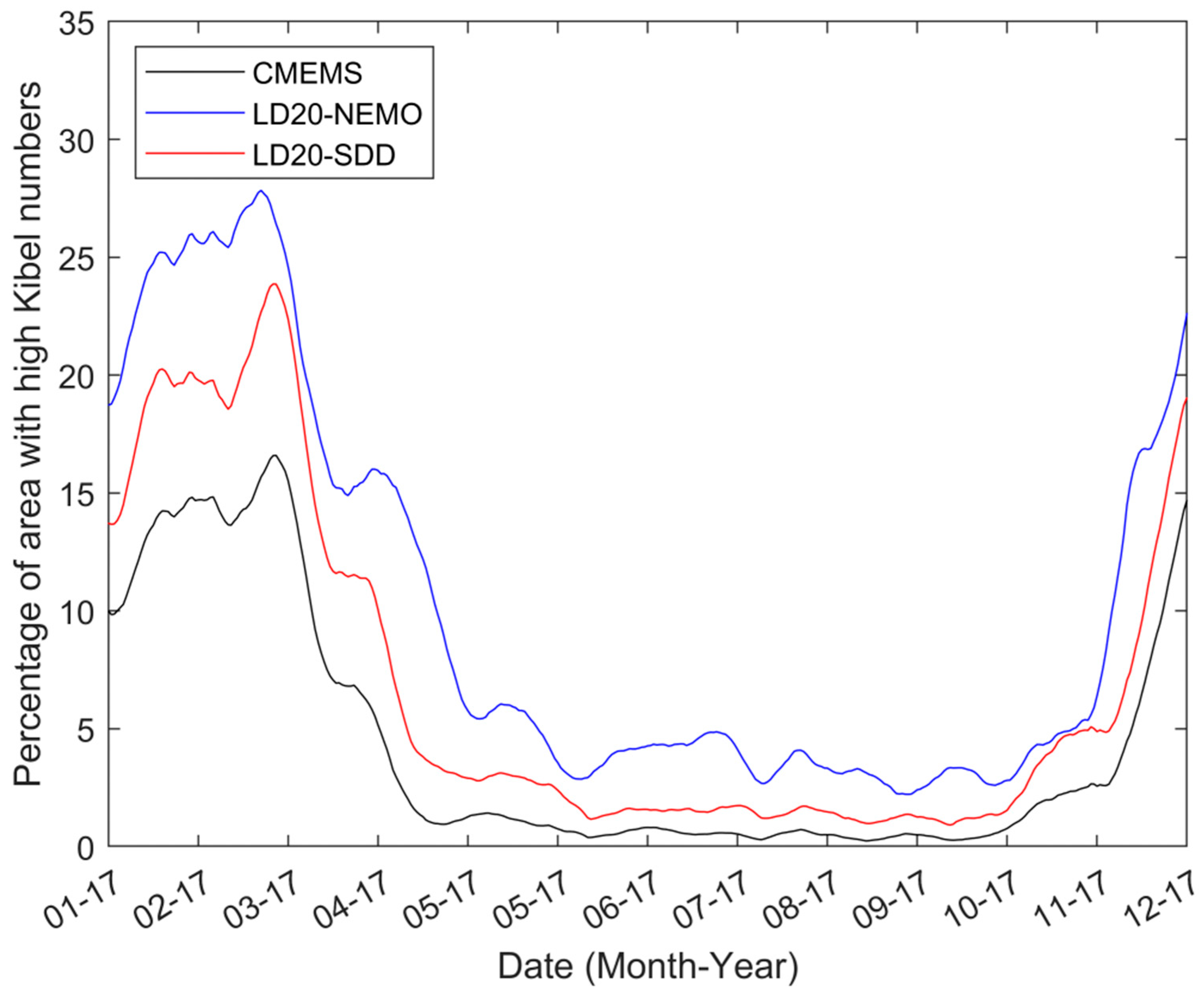
In order to separate areas of high and low non-linearity in the ocean dynamics, we set a threshold value of the Kibel number, Ki = 0.5. Figure 9 shows the time series of the Kibel number for the year 2017, which revealed that the mesoscale activity exhibited strong seasonal variability, being higher in winter–early spring. Similar variability was detected in the other years studied.

Figure 10 below shows the maps of high (Ki > 0.5) and low (Ki < 0.5) non-linearity in the Lakshadweep Sea in winter and summer. These periods were selected to show two contrasting seasons. The highest and lowest percentage of areas occupied by non-linear dynamics were produced by LD20_NEMO and CMEMS, respectively. The LD20_SDD model produced intermediate values. It was likely that CMEMS underestimated the size of high non-linearity areas due to insufficient resolution. In winter and early spring, the area occupied with highly non-linear processes could be as high as 20% or more of the whole Lakshadweep Sea.

The computational efficiency of the higher-resolution models was as follows. For LD20-NEMO, one model day of simulation took 2.5 min on 96 computing cores of an HPC cluster. LD20-SDD was run on a single core of an office Windows PC. It also took 2 min to simulate one model day, the speed was mostly dependent on the speed of reading and writing data to the disk storage. Therefore, the LD20-SDD model was approximately 100 times more computationally efficient than LD20-NEMO.

4. Discussion

The need for higher resolution ocean modelling has been identified in several areas of research. The study of mesoscale and sub-mesoscale dynamics in the Gulf of Aden was much improved when 5 km and 1.5 km resolution models were used, even though the baroclinic radius of deformation was in the range of 40 to 50 km [41].

The increase in ocean resolution in global coupled models, where the ocean component explicitly represents transient mesoscale eddies and narrow boundary currents, was shown to improve the coupled ocean–atmospheric model and produce a better weather forecast [42]. The uncertainty of climate models is partially attributed to the insufficient resolution of their ocean component [43,44], however, the refinement of model resolution is associated with significant increase in computational cost [42]. In this study, we provided a comparative skill test for two ocean models of the same resolution, LD20-NEMO and LD20-SDD. The former was based on the widely used deterministic approach, while the latter was based on the new stochastic–deterministic methodology and was significantly faster, by a factor of about 100. The models were set up to study the Lakshadweep Sea, which is known for its dramatic seasonal change of general circulation and intensive mesoscale dynamics, in particular around the southern tip of India [45]. The Lakshadweep Sea is an important source of food supply for India, Sri Lanka and the Maldives [46], and the efficiency of fishery is reliant on the smaller scale phenomena such as variations in the coastal current and upwellings.

At a glance, the NEMO and SDD versions of the LD20 Lakshadweep Sea model seem to be very different. LD20-NEMO is based on the laws of physics implemented as deterministic equations, whilst LD20-SDD is entirely data driven. At a deeper level, these models have some common features. Scientific laws are generalizations about a range of natural phenomena, sometimes universal and sometimes statistical [47]. An example may be the immense catalogue of astronomical observations giving the positions of about 1000 stars, collected by Tycho Brahe over many years. Brahe’s observations were then consolidated in Kepler’s laws of planetary motions and then further generalised by Isaac Newton as the law of gravity. However, due to the limitations of the purely deterministic approach, the equations used in ocean modelling must be supported by observations, for example, in the form of data assimilation. The limitations for the equations of motion for ocean modelling are dominated by resolution issues and ultimately by the very small scales of oceanic turbulence. In addition, adequate representation of boundary condition and initial conditions as well as other issues are important, see [48]. Data assimilation improves the output of a deterministic model by using statistical properties of differences between the model and observations.

In contrast with data assimilation, the SDD method is concerned with the statistics of the external data, alone. The practical statistical parameter used in SDD is the correlation length between fluctuations of field variables. Dynamical processes in the ocean are interconnected, and the field variables may have a number of correlation lengths reflecting different processes. The purpose of the SDD method is to reconstruct the meso- and sub-mesoscale structure of the field variables, which is only embryonically seen in the coarser parent model. The typical size of mesoscale features, such as eddies or filaments, is determined by the baroclinic radius of deformation, usually of the first or second mode [49,50]. If the non-linearity parameter of a mesoscale eddy $r=\frac{U_{orb}}{C_{phase}}>1$ (where $U_{orb}$ is the maximum orbital velocity in the eddy, and $C_{phase}$ is the phase speed of Rossby waves) then the eddy has an inner core which traps fluid in highly correlated motion, and the outer ring continuously entrains and sheds fluid [51]. As the non-linearity parameter reduces, the inner core becomes smaller. The core of an eddy also becomes smaller if the eddy is embedded in a shear flow [52]. Therefore, the area of highly correlated field variables is likely to be smaller than the area determined by the radius of deformation. This result was consistent with our calculations. In this study, the correlation length was calculated using a two-scale approach [22]. Only the shorter (i.e., mesoscale) length scale was used for further computations, as larger scale structures were well resolved by the coarser parent model. The mesoscale correlation length in the Lakshadweep Sea was typically in the range of 15 to 60 km (see Figure 3). As expected, it was lower than the first baroclinic radius of deformation in the deep Lakshadweep Sea ranging from approximately 80 to 100 km [53].

The skills of both NEMO and the SDD version of the LD20 model were assessed using the standard methodology, namely, by estimating biases, two variants of RMS errors, and the correlation coefficients between the models and observation data sets. A similar comparison was performed between two alternative observational data sets, namely, (i) GHRSST-MUR and (ii) OSTIA, which serves as a reference for judging the skills of the LD20 models. Both LD20 models performed well, showing the deviations from the reference OSTIA data within the same range as the CMEMS re-analysis and GHRSST-MUR observational data set. However, the SDD model showed slightly better performance in terms of all skill-defining parameters. The discrepancy between LD20_SDD and OSTIA was similar to, and sometimes better than, the differences between the observational data sets, GHR-MUR and OSTIA, except for the Bias. The similarity of the Bias between the LD20-SDD and OSTIA was not surprising because it was part of the design of the SDD method [8]. However, the discrepancy shown by nonlinear metrics (RMSD and RMSDA) could be higher for the finer resolution models than for CMEMS. The reason for this was that the finer resolution model may have greater gradients and/or be prone to the ‘double penalty effect’. For example, a finer resolution ORCA12 model had larger forecast errors compared with the coarser ORCA025 in regions of high temperature gradients [54]. The area and time-averaged Bias between any of the three models and OSTIA was higher than between the observational data sets.

The spatial distribution of variables demonstrating dynamic properties of the ocean state, such as current velocities, vorticity and enstrophy, is an important outcome of an ocean model, either hydrodynamic or stochastic. The maps of current velocity from all three models (see Figure 7) showed the difference in the spatial patterns produced by different modelling approaches. CMEMS is data assimilating but at lower resolution; LD20-NEMO is a dynamic model at higher resolution and has no DA; LD20-SDD is a stochastic model at higher resolution and has no DA, see Figure 7a,c,e. The difference between the models in representing currents was further clarified by the maps of enstrophy, the variable which is more sensitive to meso–sub-mesoscale variations in the ocean current gradients, see Figure 7b,d,f. In addition, the time series of surface current enstrophy was presented in Figure 8, which showed a systematic difference between lower and higher resolution models. We compared the full velocities rather than only their geostrophic components, as the Lakshadweep Sea is an area of strong ageostrophic currents, as shown in Figure 9. The computations of vorticity and enstrophy showed a greater difference between the lower-resolution CMEMS and higher-resolution LD20 models. The underestimation of vorticity by CMEMS was likely to have been caused by ‘representative error’ [55], which is related to the underestimation of sharp small-scale gradients due to insufficient resolution. The ‘representative error’ was shown to be reduced by the SDD method, which is capable of partial reconstruction of extreme values of a variable which are missed on a coarser grid [8]. It would be beneficial to validate models against velocity observations in addition to the modelled inter-comparison presented in Figure 7, Figure 8 and Figure 9, however, we were not aware of observations of surface currents or sea surface height with the required resolution to perform model-to-observation comparisons. For example, a reputable source of data [56] warned against the use of their SSH data sets for research purposes.

Both SDD and NEMO versions of LD20 showed higher values of enstrophy. The level of non-linearity of meso- and sub-mesoscale dynamics was assessed by the temporal and spatial variability of the Kibel number. A higher Kibel number is associated with relatively higher ageostrophic components of current velocities. In areas of high Kibel number, the geostrophic formulas which are usually used to infer the surface currents from satellite-derived sea level height [57] may result in large errors. The areas of highly non-linear dynamics (i.e., with a Kibel number larger than 0.5) occupied as much as 20–25% of Lakshadweep Sea in early spring, and as low as 5% in summer. The seasonal variability of the size of highly dynamic areas was consistent between all three models; while the LD20_NEMO produced the highest estimate (up to 28% in 2016), LD20_SDD produced a slightly smaller figure (up to 26% in 2017), and the lower resolution CMEMS produced the lowest figures, of up to 18% in 2017.

In summary, all three models produced a similar representation of the area-averaged values and temporal evolution of temperature and salinity. The benefit of higher resolution models comes into play in simulations of gradient-dependent values, such as vorticity and enstrophy. Both versions of LD20 showed higher values of vorticity and associated parameters than the coarser resolution CMEMS. The NEMO version of LD20 produced slightly higher values of enstrophy than the SDD version, however the SDD model was approximately 100 times more efficient computationally. It was difficult to judge which version of LD20 would produce more realistic fields of vorticity at smaller scales as we were not aware of any current velocity observations with comparable spatial coverage and resolution.

5. Conclusions

In this study, we compared the skills of three ocean models, the parent model CMEMS run by EU Copernicus Marine Service at 1/12° resolution, and two child models, LD20_NEMO and LD20_SDD run by Plymouth Ocean Forecasting Centre, both at 1/20° resolution. LD20_NEMO was based on the deterministic approach while LD20_SDD used the stochastic properties of the field variables assessed from the outputs from the parent model. All three numerical models showed similar skills in reproducing temperature and salinity assessed against observations. As expected, higher resolution models better resolved smaller scale processes. This difference was particularly significant in simulation of vorticity fields and computation of the share of the sea occupied by highly non-linear processes. The lower values of vorticity and enstrophy by the coarser CMEMS model was likely to be caused by underestimation of sharp small-scale gradients due to insufficient resolution. We found that the SDD model was more computationally efficient than the NEMO model, by a very large margin.