Analysis of Flow Field Characteristics of Aquaculture Cabin of Aquaculture Ship

Abstract

To investigate the influence of the number of inlet pipes on the characteristics of flow field and the discharge of solid particles such as bait residue and fish feces, STAR-CCM + was used to analyze the flow of field distribution in a ship-based aquaculture cabin under the conditions of two and four inlet pipes, thus optimizing the inlet pipes of the ship-based aquaculture cabin. Furthermore, a three-phase flow model (solid–liquid–gas) was established to determine the movement characteristics of similar solid particles of residual bait and fish manure in the cabin, while the emission performance of solid particles was analyzed. Finally, the formation of solid particles in the center of the aquaculture cabin was simulated. The simulation results show that the effect of flow field is better with two inlet pipes, and the discharge volume of the bottom outlet has little impact on the emission of solid particles. Findings from this study can serve as a reference and basis for the design and optimization of the aquaculture cabin of an aquaculture vessel.

1. Introduction

With the significant increase in global seafood demands in recent years, the aquaculture industry has expanded rapidly to contribute to more than half of the overall fish production worldwide [1]. However, the wastewater from offshore aquaculture has a bad impact on the environment, such as heavy metal pollution and eutrophication [2]. Therefore, the further expansion of aquaculture to the deep sea is imperative so as to enable sustainable development [3]. The mobile aquaculture vessel has good self-propulsion and a closed aquacultural environment, thus, more and more aquaculture vessels are used in the deep-sea aquaculture industry. Since fish farming requires a high-quality flow environment, there are certain requirements for the inlets, outlets, and flow velocity of the aquaculture cabin. Therefore, many scientists have conducted experimental and numerical simulation studies in this field.

In 2004, Joan et al. [4] compared the distribution of the flow field in rectangular aquaculture ponds under different inlet structures. The results showed that the horizontal tangential inlet could achieve higher and more uniform flow velocity, thus preventing the deposition of solid particles. In 2006, Lunger et al. [5] suggested that the impact of fish on aquaculture pond hydrodynamics should be given more consideration in aquaculture pond design, as different species can have different impacts. In 2007, Oca et al. [6] analyzed the simplest inlet and outlet configuration to create a uniform rotating flow pool in a rectangular aquaculture pond and combine the advantages of rectangular and round ponds. They further suggested that higher velocity is critical for the self-cleaning performance of the aquaculture pond. In 2013, Lee et al. [7] studied the fluid flow in aquaculture tanks and simulated the inlet structure of tangential flow and normal flow. Davidson et al. [8], in 2015, also compared and analyzed in experiments the influence of inlet structure of a Cornell two-channel aquaculture tank on the hydraulic mixing performance and the movement of solid particles. Their study shows that an appropriate increase in the flow rate of the basin wall and bottom tends to favor the residuals, as it is beneficial to the excretion of residues. In 2017, Liu et al. [9] simulated the hydrodynamics in an octagonal aquaculture pond of a recirculating system and found that the particle removal rate in an octagonal aquaculture pond is 90%. This study therefore shows that a consistent numerical model of hydrodynamics in an octagonal aquaculture pond can be further used for its design and optimization.

In 2018, Gorle et al. [10] created a numerical model of an octagonal aquaculture pond and investigated the influence of wall drainage on large- and small-scale turbulent structures using turbulent kinetic energy and vorticity distribution. In 2021, DD Shao et al. [11] studied the use of ‘buffer‘ net panels at the end of an aquaculture cage array to reduce the hydrodynamic load on aquaculture cage arrays. In 2022, Xi Zeng et al. [12] used particle image velocimetry and planar laser-induced fluorescence technology to explore the influence of rigid material construction on aquaculture cages. They measured the flow field and concentration field in the near-wake region of a steady current through a rigid metal net panel to analyze the flow pattern and mass transport process.

The aquaculture cabin needs to be fed with a large amount of feed during the aquaculture process, and solid particles such as bait residue and fish feces can easily settle on the floor of the aquaculture cabin. If they are not disposed of in a timely manner, the aquaculture cabin will decompose and produce harmful substances that will contaminate the water and consume dissolved oxygen, which will affect the health of the fish [13]. Thus, the effective and timely emptying of solid particles such as bait residues in the aquaculture cabin is a problem that must be considered when developing a circulating aquaculture system. In addition, it is also imperative to note that the geometry of circular ponds is very common in aquaculture [14]. The hydrodynamic performance of circular aquaculture ponds is better than that of rectangular aquaculture ponds, and rectangular aquaculture ponds are still widely used because of their easy operation [15]. In summary, an octagonal aquaculture cabin on a ship is designed as the analysis object in this paper. According to the simulation results, the solid-particle emission efficiency of the ship-borne aquaculture cabin exceeded 90% This model is helpful to solve the problem of solid-particle excretion in marine aquaculture.

In this paper, the characteristics of the flow field of two and four inlet pipes in each area of the aquaculture cabin are calculated under different working conditions. This is performed by comparing the average velocity and uniformity of the flow field in the cabin before the optimal arrangement of the inlet pipes is determined. Furthermore, a numerical phase of the liquid–gas–solid technique was adopted using a turbulence model and a multiphase flow model, which was established to investigate the system trajectory, drainage time, and emission efficiency of solid particles such as residual bait and fish manure in the aquaculture chamber while observing its influence on the hull movement.

2. Model and Principle

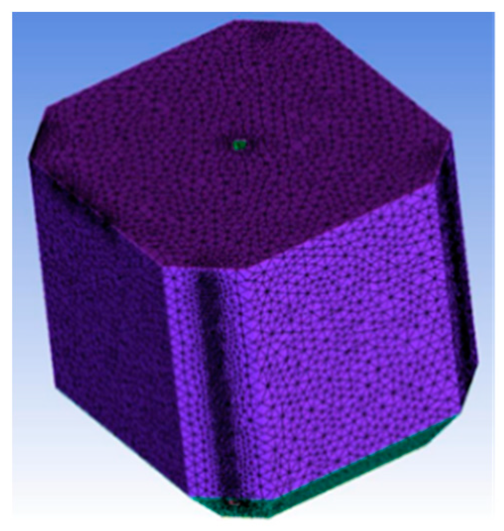
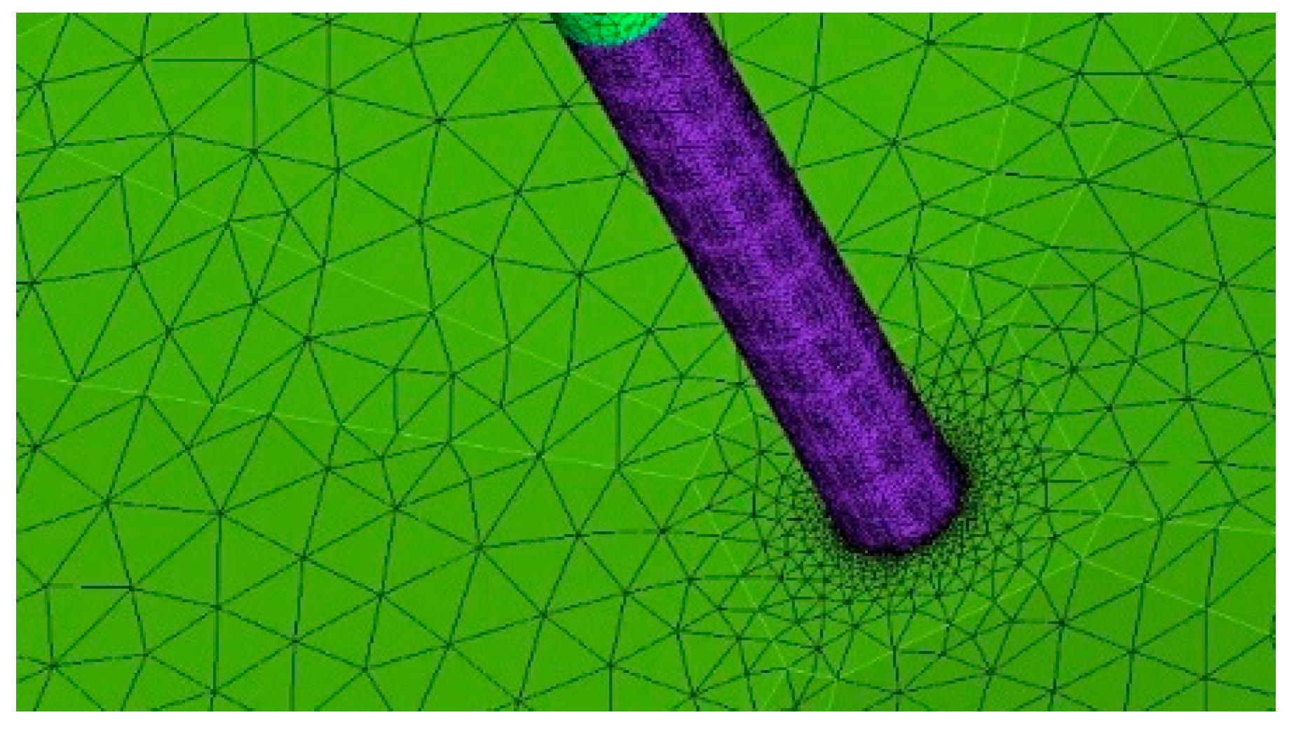
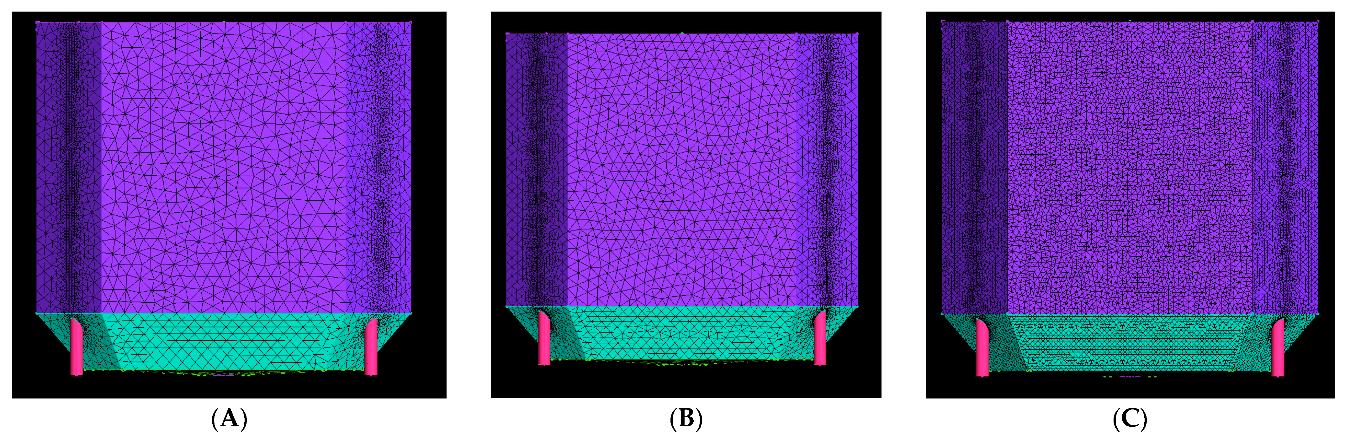
2.1. Geometric Model and Meshing

There are 18 aquaculture cabins on the aquaculture ship, and the typical aquaculture cabin (aquaculture cabin No. 7) is taken as the research object, as shown in Figure 1. The length, width, and height of the aquaculture cabin are 15.34 m × 16.60 m × 17.00 m, respectively, with 33 round holes arranged in the vertical direction of the inlet pipe, and the diameter of the round hole can be adjusted according to the flow rate. The space of the aquaculture cabin was divided into grids, and the details of the inlet and outlet were calculated. The grid distribution is shown in Figure 2, Figure 3 and Figure 4, and the total grid number of the aquaculture cabin is 2.6 million. The grid number for the water inlet pipe is 107,300 and the grid number for the water inlet is 137,000. The grid number for the water outlet pipe is 56,000, while the grid number for the middle pipe outlet is 15,000. Finally, the grid number for the bottom outlet is 35,000 and the grid number for the top outlet is 26,000.

2.2. Grid Independence Verification

To exclude the influence of mesh density on the simulation results from the flow field in the aquaculture cabin, the mesh independence was tested in this study. The grid of the whole aquaculture cabin and its geometric model is shown on the right of Figure 1. The mesh size was reduced by 25% each time, and the corresponding mesh numbers were 1.26 million, 2.85 million, and 6.42 million, respectively. Three groups of grids with different densities were designated, as shown in Figure 5. The average velocities of the flow field were calculated with the three groups of grids and they were sorted out for comparison. The comparison results are shown in

Table 1. Average velocity results at different locations.

Position (m)	Speed (m/s)
H = 5	(A) 1.26 million 0.101	(B) 2.85 million 0.121	(C) 6.42 million 0.112
H = 10	0.098	0.103	0.109
H = 15	0.099	0.101	0.106
Entire flow field	0.099	0.108	0.109

. H is the height from the bilge.

It can be seen from the calculation results in Table 1 that the average velocity of the entire flow field is not very different between (B) and (C), so the mesh density has little effect on the calculation results.

2.3. Turbulence Model

The RNG ‘k-ε’ turbulence model was chosen as the flow model in this study. Compared to the standard ‘k-ε’ turbulence model, this model has significant advantages in handling flows with high strain rate and strong streamline curvature [16]. The RNG ‘k-ε’ turbulence model corrects the turbulent viscosity, taking into account the anisotropy of the turbulence in the actual situation and the rotation as well as the average rotational flow, where the generation term is related to the flow and spatial position. Due to the above improvements, the RNG ‘k-ε’ model achieves more accurate results than the standard ‘k-ε’ model [17,18].

2.4. Multiphase Flow Model

For the numerical calculation and analysis of solid particles, the discrete phase model (DPM) was chosen, where the fluid is treated as a continuous phase and the solid particles as discrete phases. The statistics of the solid particles are obtained by solving the DPM [19,20,21]. When the influence of rolling motion is considered, the flow field is calculated using Euler multiphase flow (liquid–gas). The free surface area of liquid–gas is calculated using the volume-of-fluid method, while the trajectory of the particles is tracked using the Lagrangian [22] approach. The solid particles included in the calculation are mainly fish dung and bait residues. The physical properties (density, etc.) of these solid particles are difficult to measure. In this study, the physical properties of similar solid particles are used instead. The volume fraction of solid particles in the liquid of the breeding tank is about 0.038%, much less than 6.5% [23], and the influence of solid particles on the flow field is insignificant and not considered.

2.5. Calculation Parameter Selection

The numerical simulation is performed using the simulation software Star CCM + and the implicit transient control method is chosen to solve the DPM. The solid–liquid coupling is considered for the solid phase model to simulate the deposition and operation of solid particles [15]. The discrete phase solid particles consider gravity, resistance shear lift, etc. The relevant parameters are shown in

Table 2. Solid particle parameter table.

Fluid Density	Fluid Viscosity	Concentration of Solid Particles	Density of Solid Particles	Elastic Coefficient
1025 kg/m3	1.21 7 × 10−3 Pa·s	40 mg/L	1050 kg/m3	0.5

. The interaction between the particles and the solid wall is defined as an incomplete elastic impact, and the elasticity coefficient is set to 0.5. Initially, the flow field is assumed to be a uniform static flow field and the relative pressure is 0. The initial velocity field is 0. The wall surface (cabin wall, pipe wall, etc.) is set as the ‘wall’ boundary. The inlet pipe is set as the velocity inlet boundary, and the side discharge pipe is set as the outlet boundary to control the relationship between the side discharge and the bottom discharge. Finally, the bottom drainage is set as the boundary for the pressure outlet.

In addition, an ‘ejector’ technique was used with the Star CCM + software to create solid particles. Using this solid particle formation as an example, the ejector parts were generated at the edge of the incubator and the number of ejection points was determined. In this study, a 10 × 10 ejection point with a mass of 2.6376 × 10⁻³ kg was defined. The concentration in the water was 40 mg/L, the residence time of the particles was 5 h = 18,000 s, and the average mass flux was 0.056 kg/s. The initial velocity of the sprayed particles was assumed to be 0.01 m/s, while the step size was 0.01 s.

3. Results and Discussion

To investigate the emission of solid particles in the aquaculture cabin, the flow field and trajectory of solid particles were numerically simulated under the conditions of 10%, 20%, 30%, and 40% of water discharge of two and four inlet pipes, respectively. The curves of emission efficiency of solid particles under different conditions were quantitatively evaluated. By calculating the number of particles per hour, the number of particles discharged from the cabin per unit of time was calculated and the emission efficiency curve was created. Based on the results of the flow field analysis and the optimum working conditions determined by the flow field analysis, the particle emission under these optimum working conditions was calculated and simulated. This paper also discusses the particle emission of the aquaculture cabin on the ship under the rolling conditions when operating at sea, and the results of the calculation simulations under each operating condition are shown below.

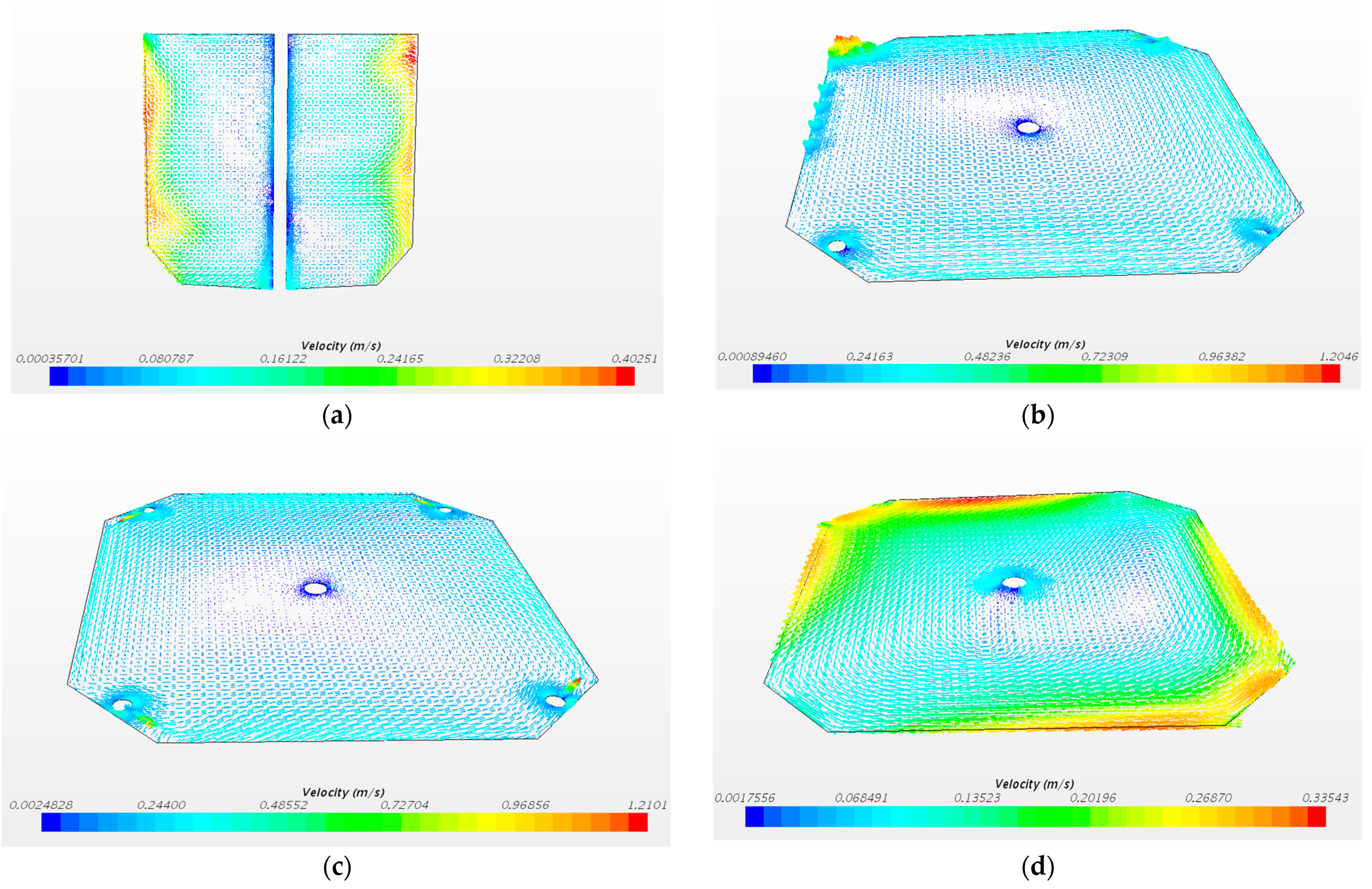
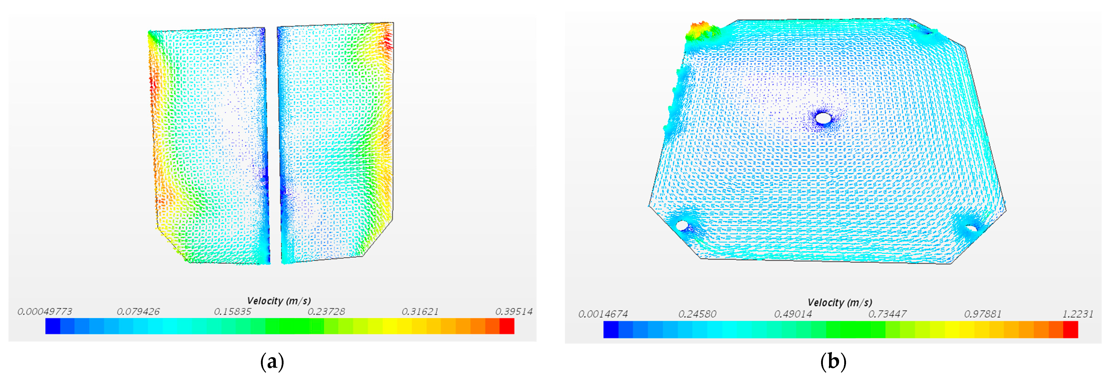
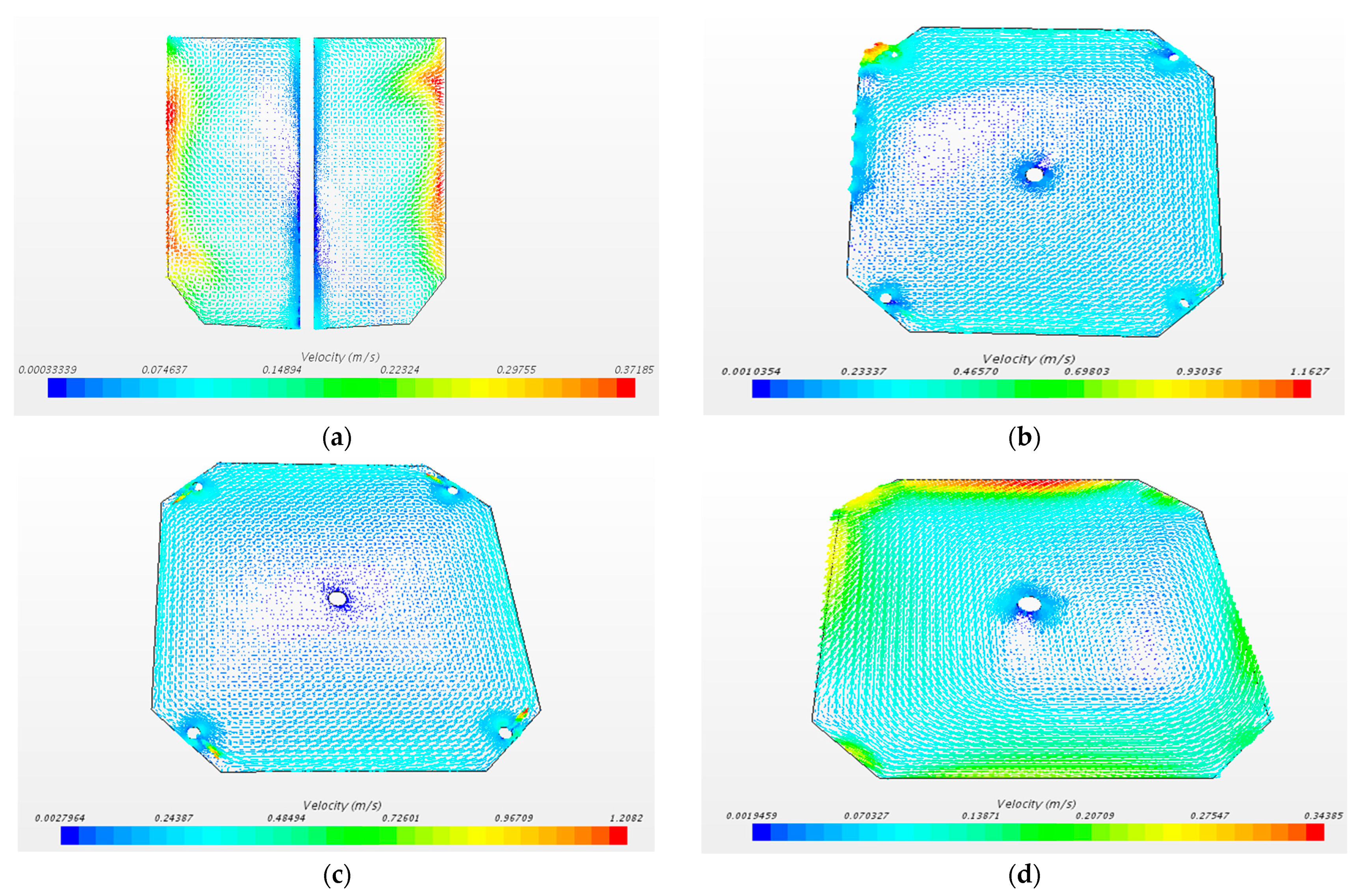
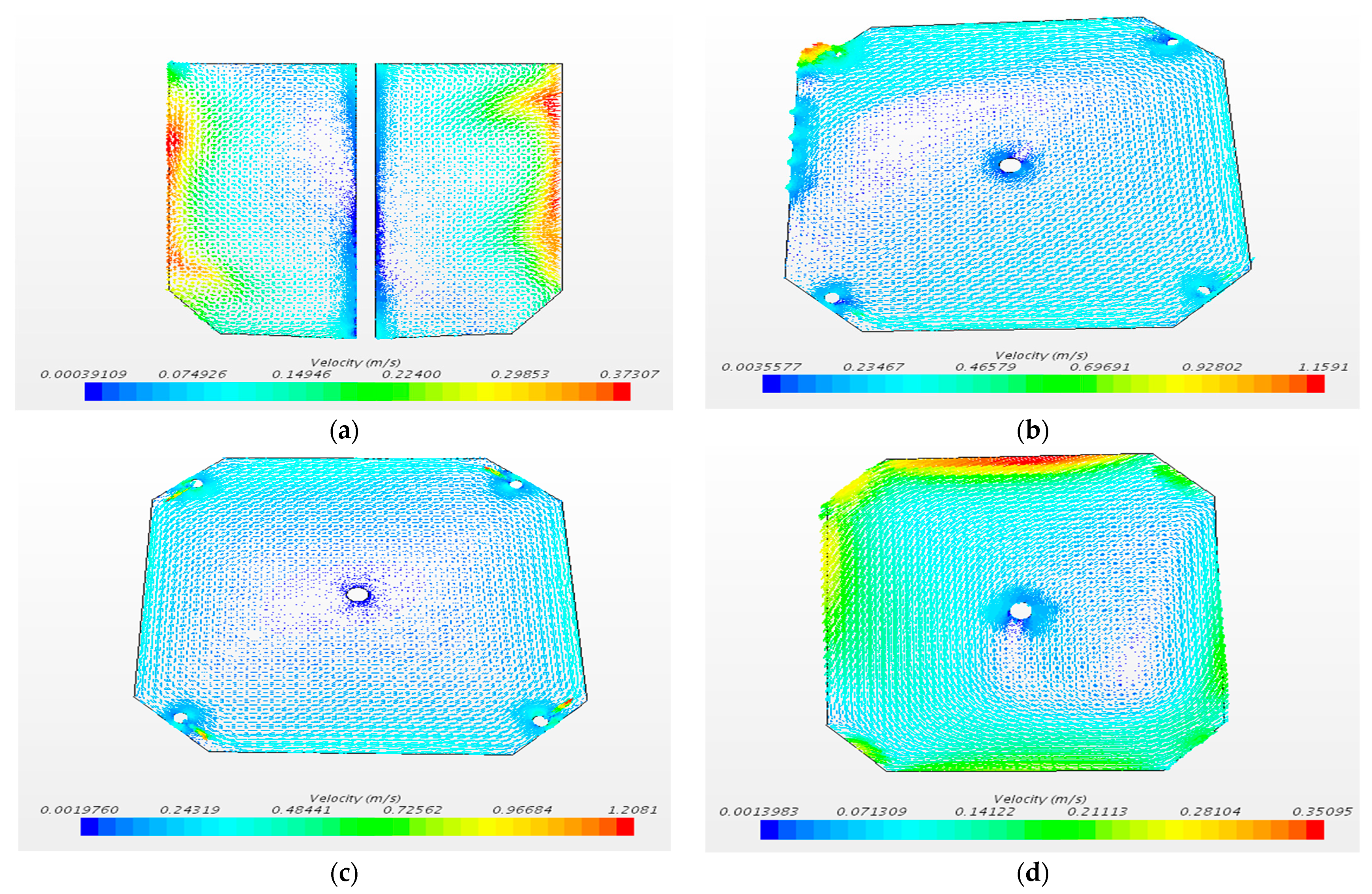
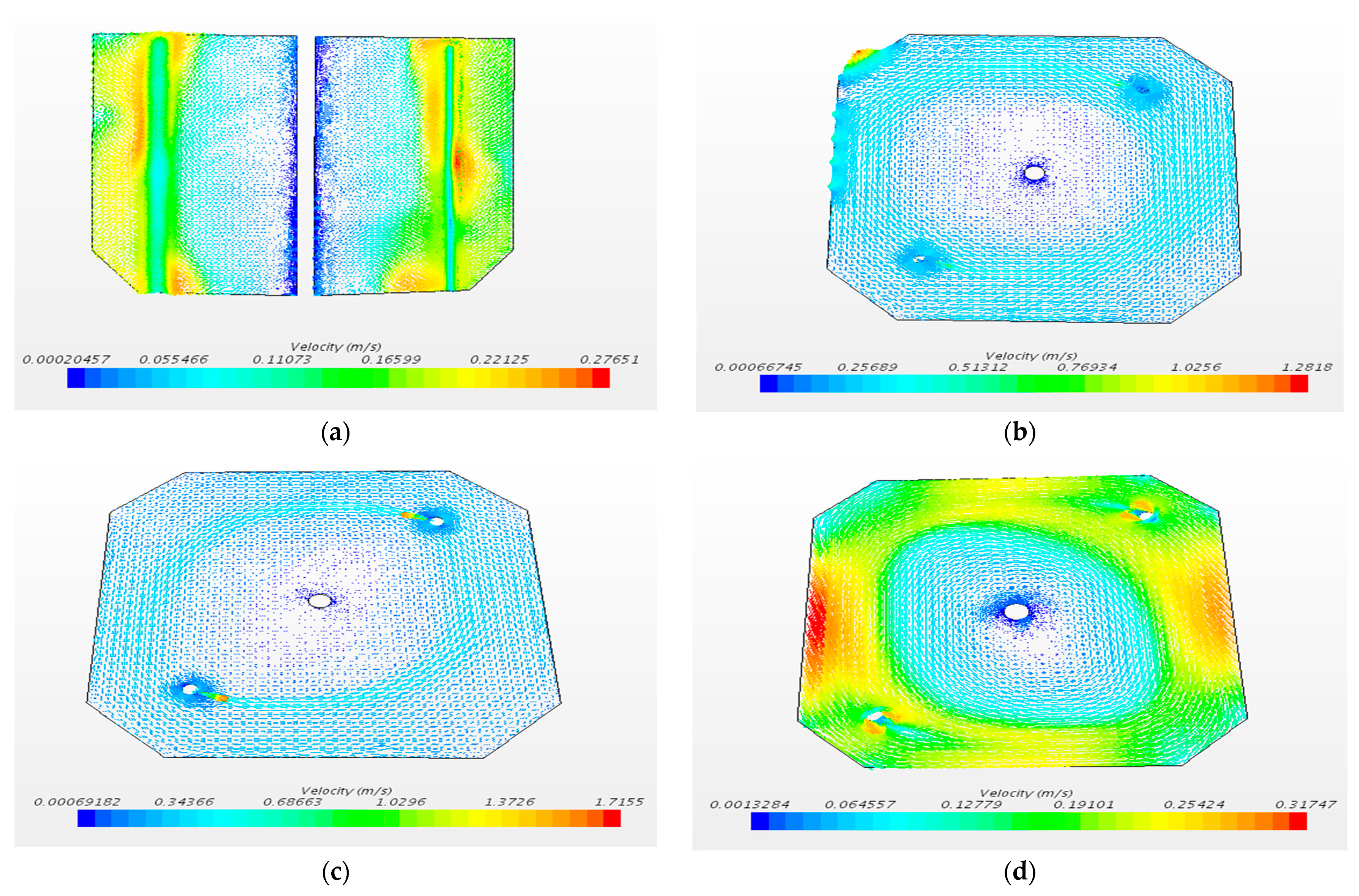
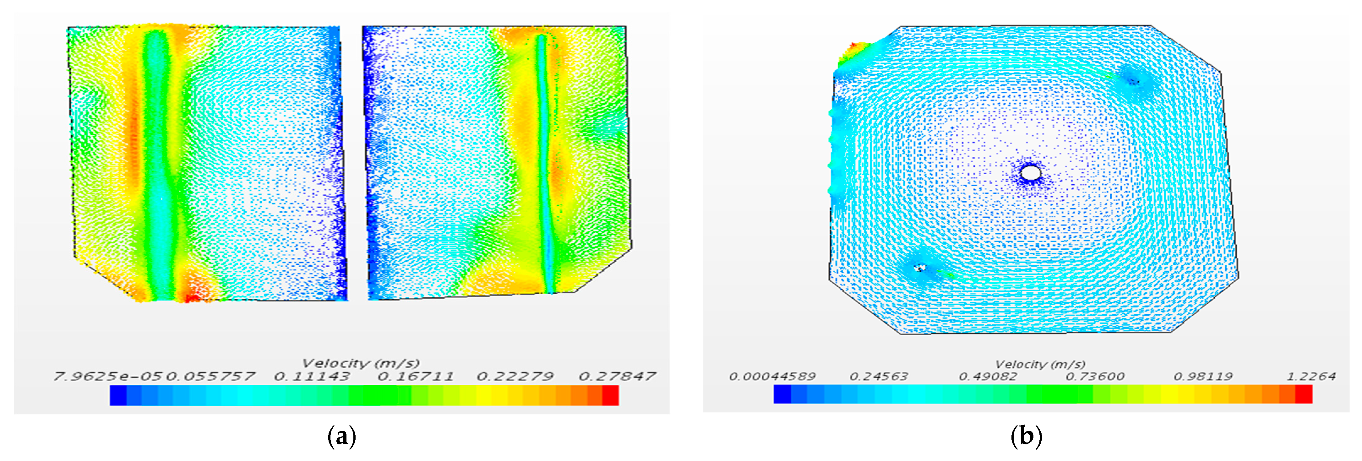
3.1. Working Condition of Four Inlet Pipes

It is assumed that the particles are all generated from the top of the aquaculture cabinet, that the inlet velocity is 100%, that the inlet velocity is 1.52 m/s, and that the discharge volume is controlled at the bottom. Based on the above Euler method and Lagrange method, the particle emission was numerically simulated at different discharge volumes at the bottom, and the trajectory of 40 particles was simply followed. When the particles move near the outlet, they are considered discharged. The number of particles discharged within 5 h was counted, and the emission efficiency of the particles was calculated accordingly. In this study, the cloud diagram of the velocity field in the longitudinal section of the aquaculture cabin (h = 16.5 m, h = 8.5 m, and h = 1.5 m) was recorded and the real-time movement diagram of particles in some moments of each working condition was obtained.

(1)

Bottom outflow ratio of 40%

As shown in Figure 6, the particle emission process in the cabin was simulated and the velocity field at four cross-section positions in the cabin was intercepted under the condition of 40% drainage at the bottom of the aquaculture cabin.

Assuming that the particles are generated from the top, the position of 40 particles in the cabin within five hours was simply tracked. It can be seen from the Figure 7 that the number of particles in the cabin decreases with time. When the particles move to the outlet attachment, they are considered to be discharged, and the discharge efficiency of the particles is calculated accordingly.

(2)

Bottom outflow ratio of 30%

As shown in Figure 8, the particle emission process in the cabin was simulated and the velocity field at four cross-section positions in the cabin was intercepted under the condition of 30% drainage at the bottom of the aquaculture cabin.

From the Figure 8 and calculation results, it can be seen that under the conditions of 40% and 30% displacement at the bottom, there is a large velocity gradient in the flow field and the distribution of the flow field is not uniform, which is not conducive to the discharge of particles. The influence of the non-uniform distribution of the flow field on the efficiency of particle emission is greater than the influence of the change in the ground displacement on the efficiency of particle emission.

(3)

Bottom outflow ratio of 20%

As shown in Figure 9, the particle emission process in the cabin was simulated and the velocity field at four cross-section positions in the cabin was intercepted under the condition of 20% drainage at the bottom of the aquaculture cabin.

(4)

Bottom outflow ratio of 10%

As shown in Figure 10, the particle emission process in the cabin was simulated and the velocity field at four cross-section positions in the cabin was intercepted under the condition of 10% drainage at the bottom of the aquaculture cabin.

To compare and examine the effect of the change in bilge drainage on particulate matter emissions, the data in the statistical table of emission results for the four working conditions are plotted on a graph, as shown in Figure 11.

From the Figure 11, it can be seen that the change in displacement at the bottom of the aquaculture cabin has a little effect on the flow field in the cabin under the given conditions of the particles. At the same time, by comparing the emission curve of four different conditions, it can be found in the first three hours that the more the soil is displaced, the higher the emission power. In the first three to five hours, the emission efficiency depends less on the displacement and tends to be constant.

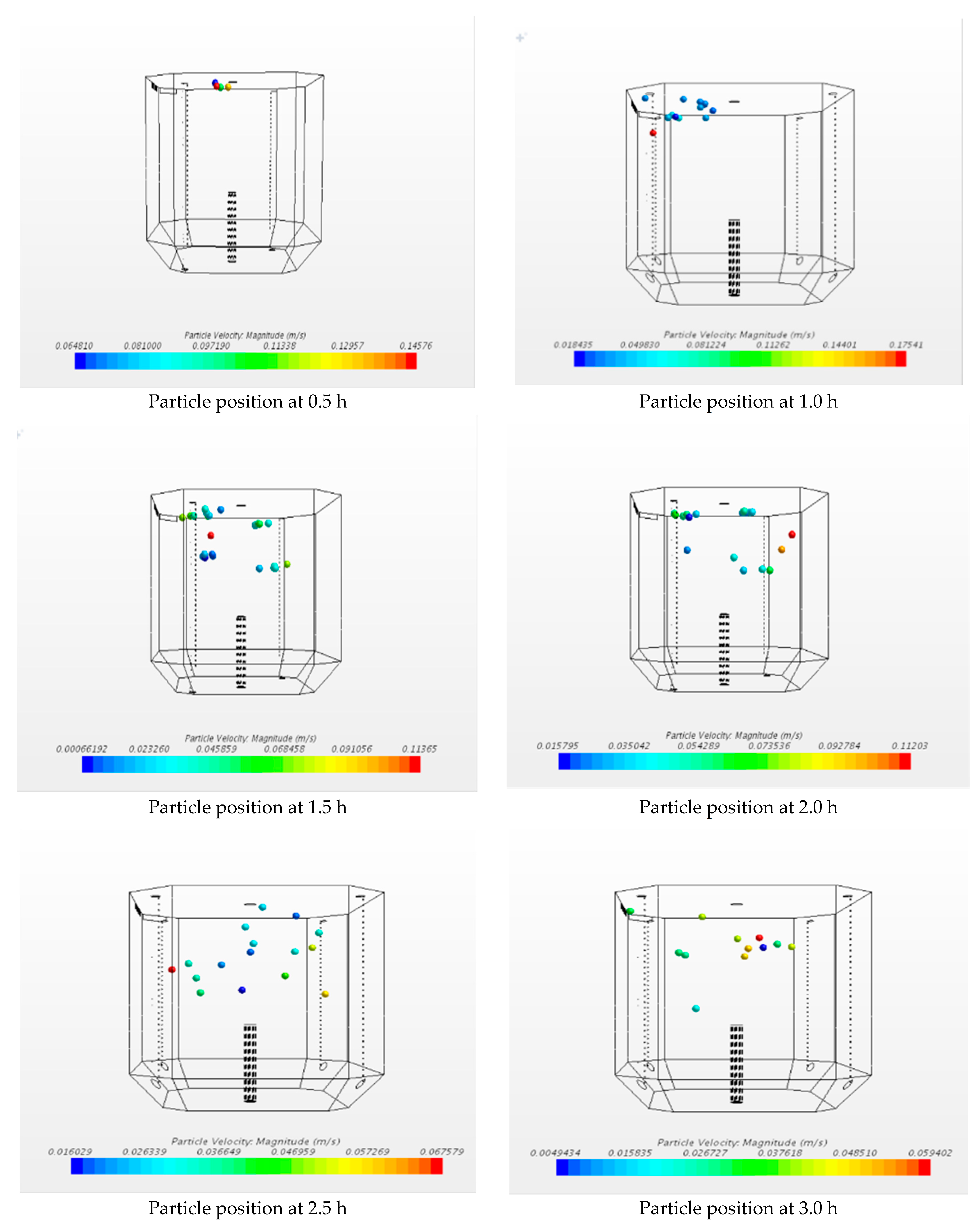
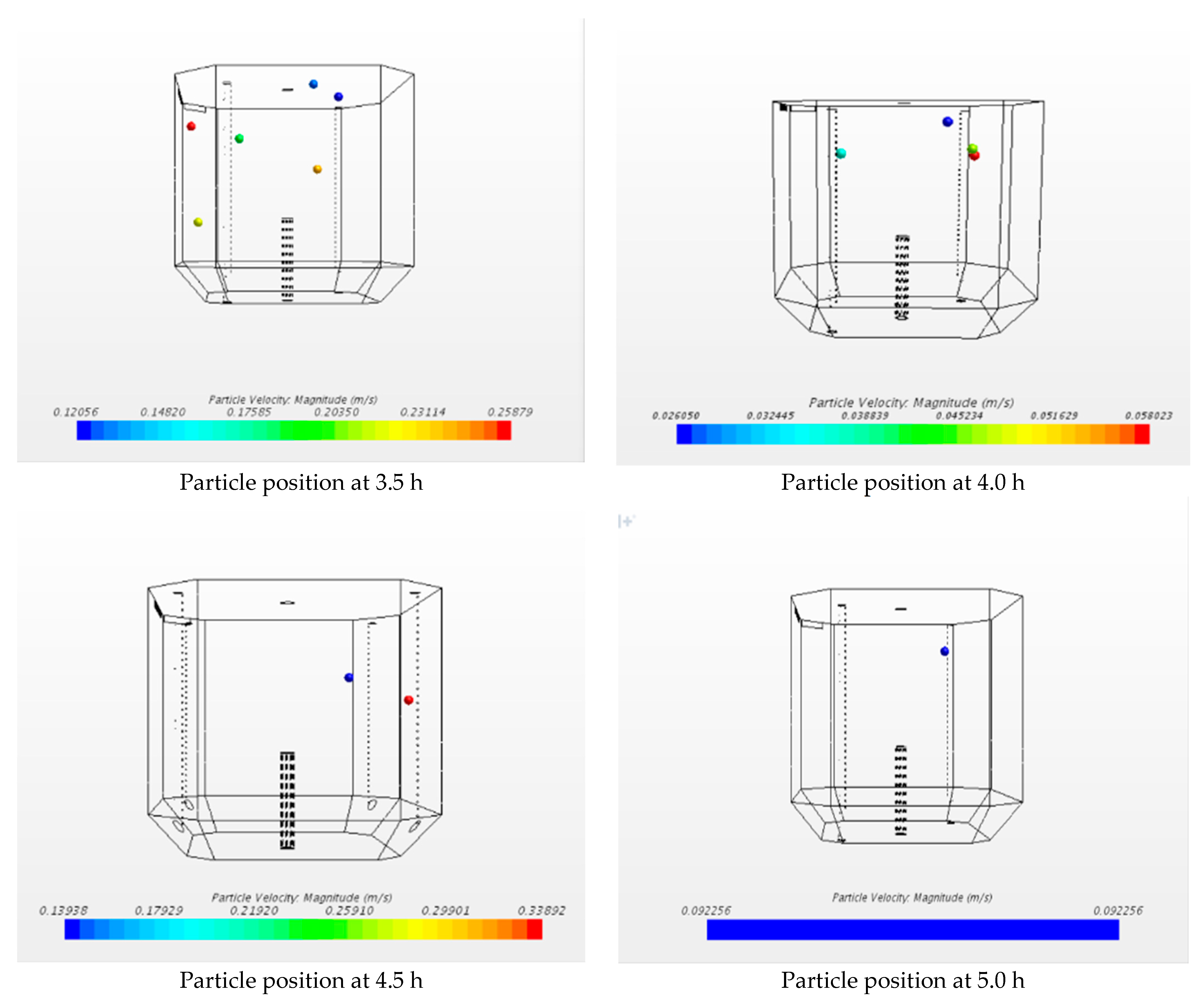
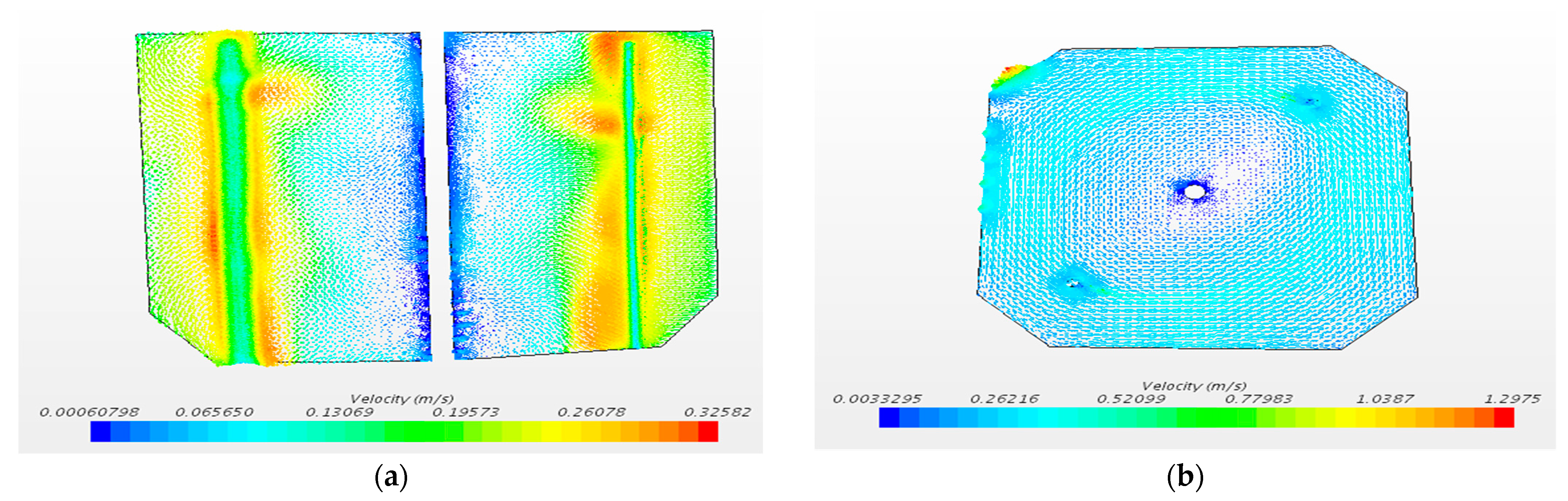
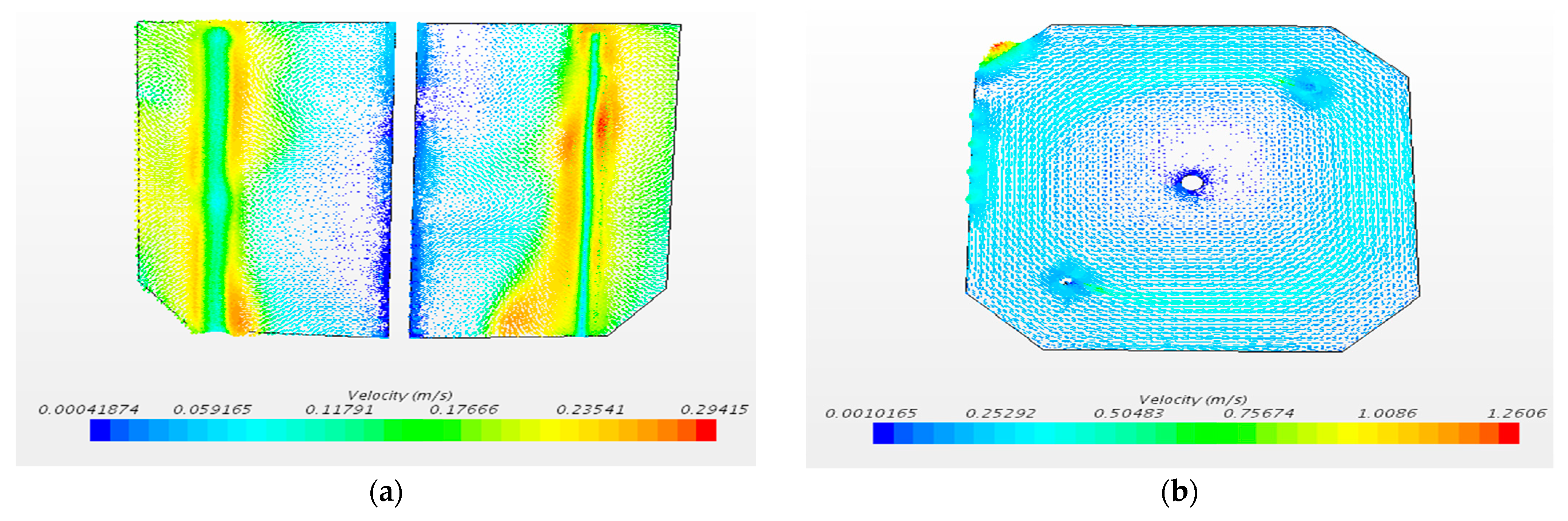
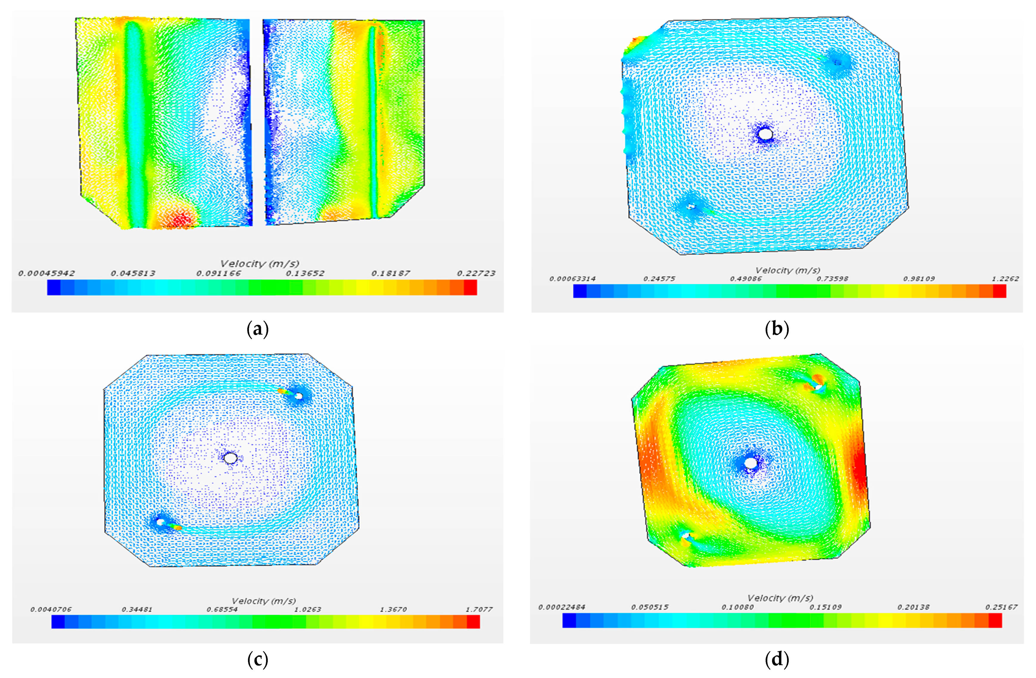
3.2. Two Inlet Pipe Conditions, Top Spray Particles

(1)

Bottom outflow ratio of 40%

As shown in Figure 12, the particle emission process in the cabin was simulated and the velocity field at four cross-section positions in the cabin was intercepted under the condition of 40% drainage at the bottom of the aquaculture cabin.

(2)

Bottom outflow ratio of 30%

As shown in Figure 13, the particle emission process in the cabin was simulated and the velocity field at four cross-section positions in the cabin was intercepted under the condition of 30% drainage at the bottom of the aquaculture cabin.

From the analysis of the Figure 13 and calculated results, it is obvious that the velocity gradient of the flow field is low, the distribution of the flow field is uniform, and the effect of particulate matter emission is better when the bottom displacements of the two inlet pipes are 40% and 30%.

(3)

Bottom outflow ratio of 20%

As shown in Figure 14, the particle emission process in the cabin was simulated and the velocity field at four cross-section positions in the cabin was intercepted under the condition of 20% drainage at the bottom of the aquaculture cabin.

(4)

Bottom outflow ratio of 10%

As shown in Figure 15, the particle emission process in the cabin was simulated and the velocity field at four cross-section positions in the cabin was intercepted under the condition of 10% drainage at the bottom of the aquaculture cabin.

In the case of the above two inlet pipes, the emission efficiency curves of the four bottom drainage volumes under different working conditions are shown in the following Figure 16.

The Figure 16 and the calculated results indicate that with two inlet pipes, the velocity gradient of the flow field is low, the distribution of the flow field is uniform, and the effect of particulate emissions seems better. Comparing the emission effect under the four conditions, we found out that the change in ground displacement has little influence on the emission effect and also has a slight influence on the emission rate, but the ground emission is large and the efficiency of the particulate emission is high.

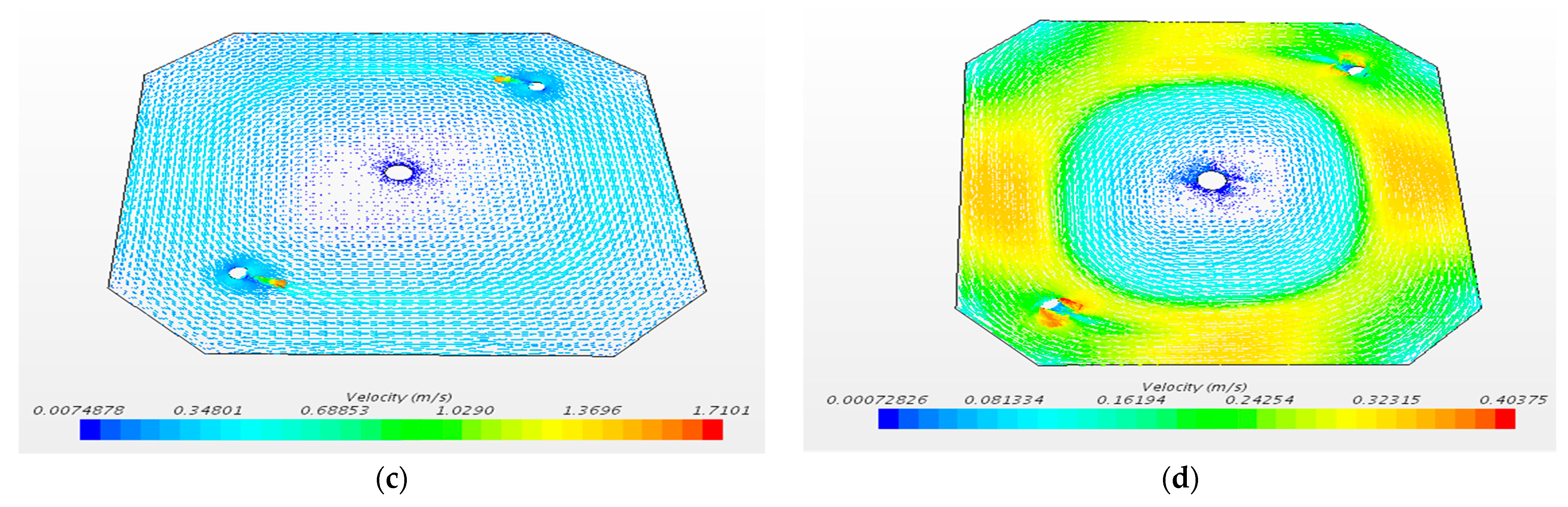
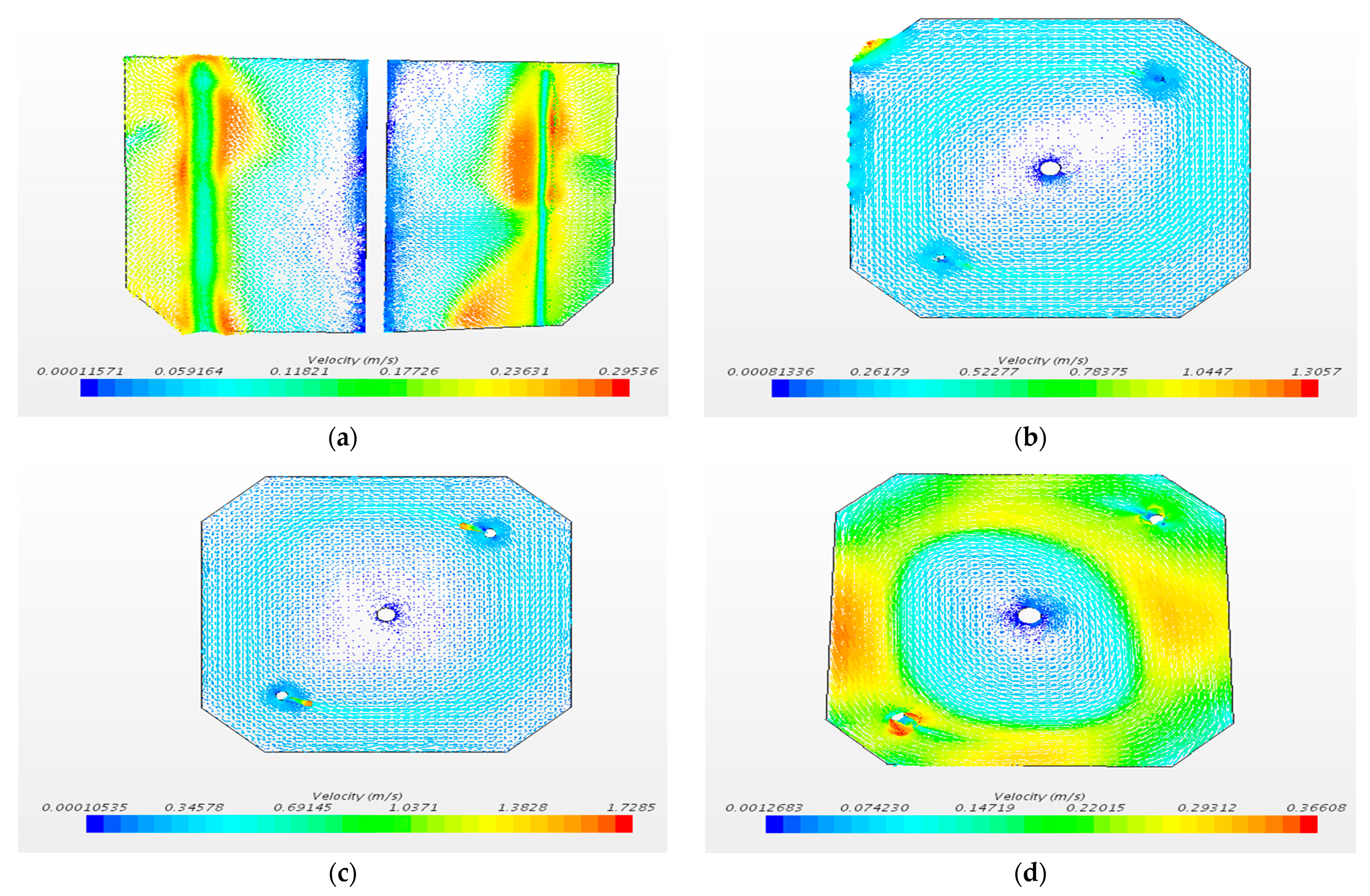
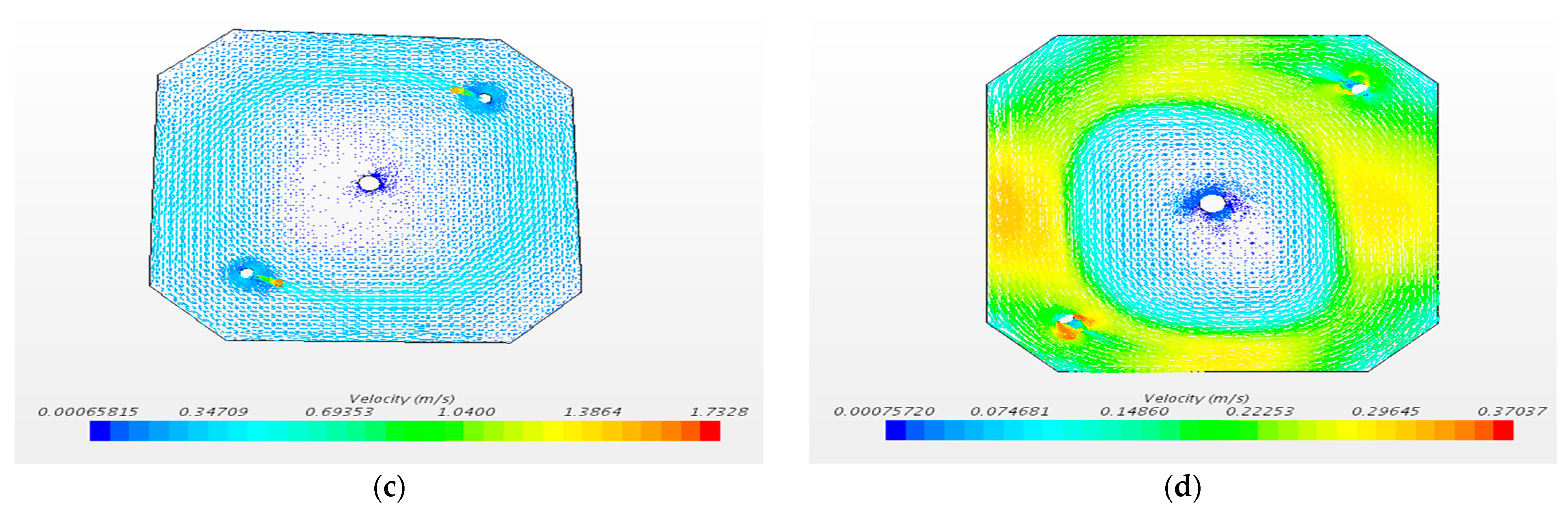
3.3. Two inlet Pipes, Central Spray Particles

(1)

Bottom outflow ratio of 40%

As shown in Figure 17, the particle emission process in the cabin was simulated and the velocity field at four cross-section positions in the cabin was intercepted under the condition of 40% drainage at the bottom of the aquaculture cabin.

(2)

Bottom outflow ratio of 30%

As shown in Figure 18, the particle emission process in the cabin was simulated and the velocity field at four cross-section positions in the cabin was intercepted under the condition of 30% drainage at the bottom of the aquaculture cabin.

(3)

Bottom outflow ratio of 20%

As shown in Figure 19, the particle emission process in the cabin was simulated and the velocity field at four cross-section positions in the cabin was intercepted under the condition of 20% drainage at the bottom of the aquaculture cabin.

(4)

Bottom outflow ratio of 10%

As shown in Figure 20, the particle emission process in the cabin was simulated and the velocity field at four cross-section positions in the cabin was intercepted under the condition of 10% drainage at the bottom of the aquaculture cabin.

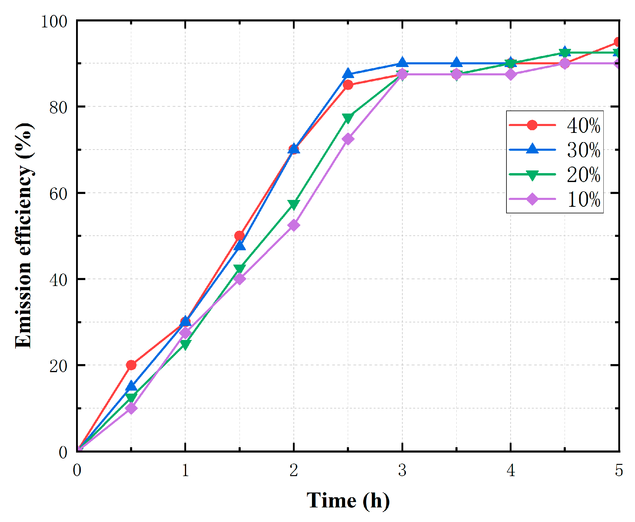
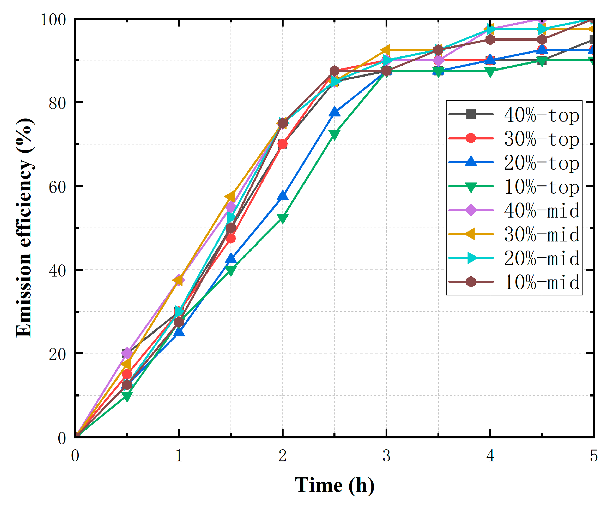
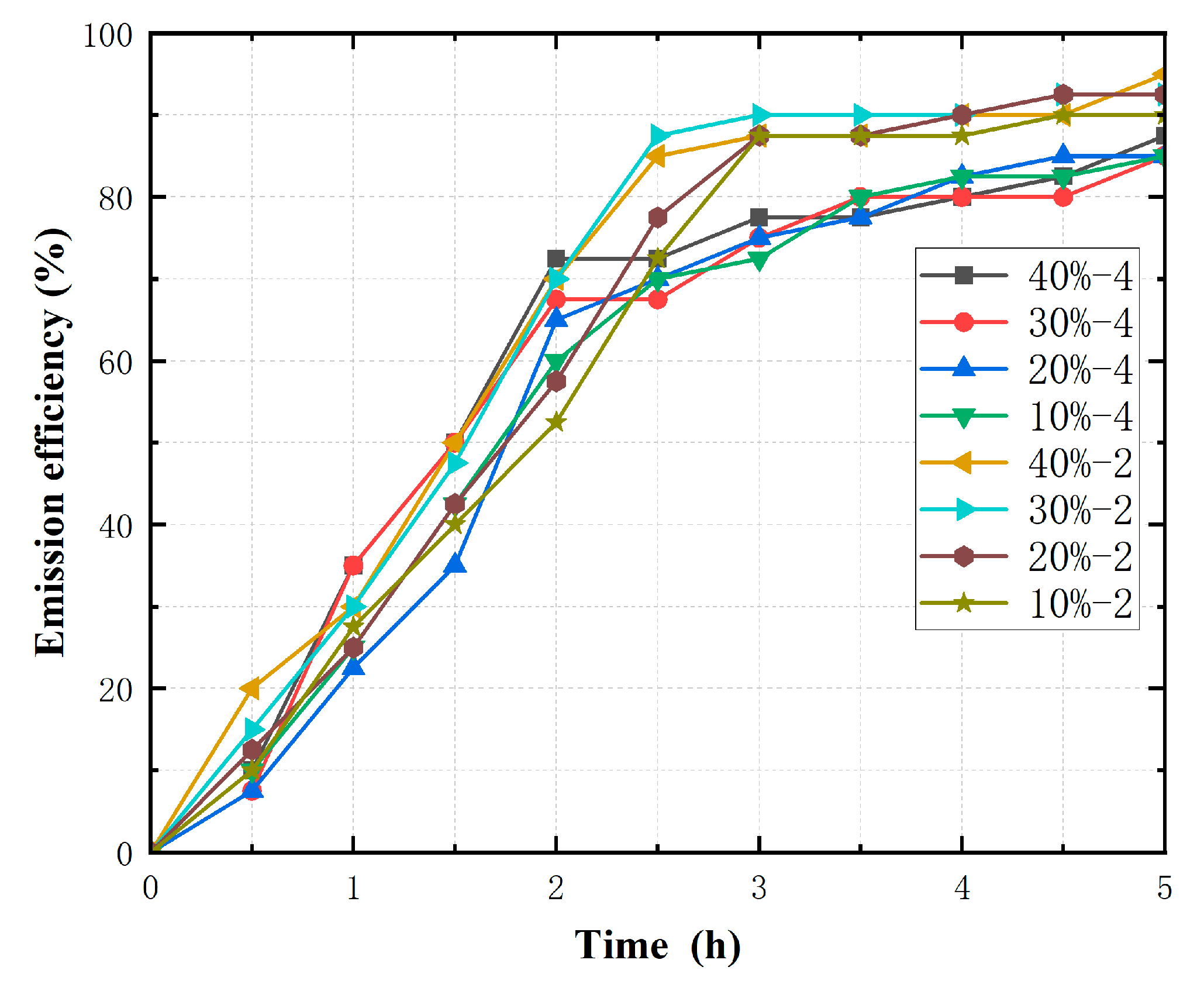
3.4. Simulation Comparison Results of Particulate Matter Emission Effect

If the location of the solid particles is in the center of the aquaculture cabin, the particles can be substantially discharged under the four working conditions. To compare the effects of the different injection positions on the emission results, we compare the particle emission results of the middle injection with those of the top injection (see Figure 21). In addition, the discharge effect of two discharge pipes is also compared with that of four inlet pipes (see Figure 22).

As illustrated in Figure 21, the initial position of the particles has some influence on their emission. The emission rate of particles produced at the center is better than that of particles produced at the top. When the inlet flow is the same, the particle emission efficiency is relatively stable and efficient under the conditions of two inlet pipes and 30% bottom discharge.

Figure 22 shows that the particle emission of two inlet pipes is better than that of four inlet pipes under the same bottom displacement condition. In conjunction with the calculation results of the flow field, it can be observed that the velocity gradient of the flow field is lower for two inlet pipes than for four inlet pipes. That is, the uniformity of the flow field is better for two inlet pipes, and the particles are less affected by the gradient force of the flow field. They are mainly influenced by gravity and air resistance, which is favorable for particle emission. Therefore, using two inlet pipes will lower the drainage rate at 30% and this conforms with the optimal conditions.

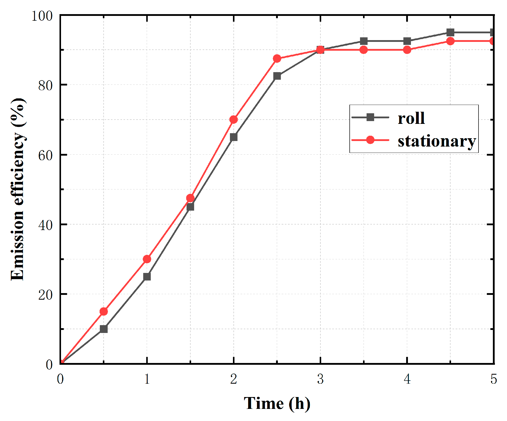
3.5. Effects of Rolling Motion

When the aquaculture cabin operates at sea, it is affected by environmental factors such as wind and waves, and there is a pendulum motion of six degrees of freedom. The rolling motion does not only pose a serious threat to the operational safety of the aquaculture cabin, but it also aggravates the non-uniformity of the water flow velocity in the aquaculture environment [24], which in turn affects the emission of solid particles. The effect of rolling motion on the emission of solid particles at different flow velocities was also simulated in this study. Taking the mild sea state as an example, this means that the wind speed is 15.5 m/s, and the significant wave height is 3.5 m, with a flow rate of 1 m/s under the parameter condition of a maximum water depth of 500 m. The flow rates at the inlet are 100%, 80%, 60%, and 40%, respectively, and the maximum amplitude of the rolling motion is 8°. The results of the comparison with the case without rolling are shown in Figure 23 below.

From the comparison of the figure, it can be observed that the emission effect of particulate matter under mild sea conditions is essentially the same as that under static sea conditions.

3.6. Effect of Different Inlet Flows on Discharge under Optimal Conditions

To compare and study the emission of particles under different inlet flow rates, the statistical results of particle emission under the above three conditions are compared with the statistical emission results under a flow rate of 100%. The comparison results are shown in the following

Table 3. Statistics of emission results at different flow rates under optimal conditions.

Detention Time (h)	100% (1.52 m/s)		80% (1.216 m/s)		60% (0.912 m/s)		40% (0.608 m/s)
0	40	0%	40	0%	40	0%	40	0%
0.5	34	15%	33	17.5%	33	17.5%	32	20%
1	28	30%	28	30%	26	35%	26	35%
1.5	21	47.5%	20	50%	19	52.5%	15	62.5%
2	12	70%	10	75%	10	75%	7	82.5%
2.5	5	87.5%	6	85%	4	90%	4	90%
3	4	90%	3	92.5%	3	92.5%	4	90%
3.5	4	90%	3	92.5%	3	92.5%	2	95%
4	4	90%	1	97.5%	1	97.5%	1	97.5%
4.5	3	92.5%	1	97.5%	1	100%	1	97.5%
5	3	92.5%	1	97.5%	0	100%	0	100%

and in Figure 24.

From the comparison of the statistical results, it can be observed that when the inlet flow rate decreases, the emission efficiency increases slightly. The reason is that the particles are mainly flowing by gravity when moving in the flow field, while the gradient force has a less significant impact on their movement.

4. Conclusions

In this paper, CFD (Computational Fluid Dynamics) is used to analyze the flow field of an aquaculture cabin of an aquaculture ship. The influence of the bilge drainage ratio and the roof drainage on the flow field of the aquaculture cabin was calculated, and the parameters of the number of inlet pipes and the installation position were optimized. According to the calculation results, a reasonable scheme is given to provide the necessary parameters for the development and design of the aquaculture cabin of the aquaculture ship, which has important engineering reference value:

(1)

The change in the discharge volume at the bottom of the outlet has a relatively less significant impact on the entire flow field, and it also has less impact on the movement of particles as well as the overall emission effect of solid particles.

(2)

The number of inlet pipe has a certain influence on the flow field and the emission of solid particles. If the aquaculture cabin is equipped with two inlet pipes under the same inlet flow rate, the emission effect of solid particles in the aquaculture cabin seems better than with four inlet pipes. This is because the flow field velocity distribution of the two pipes is relatively uniform, and the arrangement of the four pipes strengthens the annular water circulation at the four pipes in the aquaculture cabin and reduces the flow velocity inside, but the particles are mainly discharged from the middle bottom outlet. Therefore, the discharge effect of the two pipes Is better.

(3)

The initial distribution of solid particles has a significant influence on the emission effect, and if the initial distribution is in the middle of the aquaculture cabin, the emission efficiency seems better than the initial distribution at the top of the aquaculture cabin.

This study is limited by the calculation equipment, and only 5 h is counted in the numerical simulation calculation. It is recommended to supplement and improve this approach in the subsequent research work.

References

1. Yang, X.; Zeng, X.; Gualtieri, C.; Cuthbertson, A.; Wang, R.-Q.; Shao, D. Numerical Simulation of Scalar Mixing and Transport through a Fishing Net Panel. J. Mar. Sci. Eng. 2022, 10, 1511. [Google Scholar] [CrossRef]
2. Wang, X.; Cuthbertson, A.; Gualtieri, C.; Shao, D. A Review on Mariculture Effluent: Characterization and Management Tools. Water 2020, 12, 2991. [Google Scholar] [CrossRef]
3. Ma, C.; Zhao, Y.-P.; Bi, C.-W. Numerical study on hydrodynamic responses of a single-point moored vessel-shaped floating aquaculture platform in waves. Aquac. Eng. 2022, 96, 102216. [Google Scholar] [CrossRef]
4. Joan, O.; Ingrid, M.; Lourdes, R. Comparative analysis of flow patterns in aquaculture rectangular tanks with different water inlet characteristics. Aquac. Eng. 2004, 31, 221–236. [Google Scholar]
5. Lunger, A.; Rasmussen, M.R.; Laursen, J.; McLean, E. Fish stocking density impacts tank hydrodynamics. Aquaculture 2006, 254, 370–375. [Google Scholar] [CrossRef]
6. Oca, J.; Masaló, I. Design criteria for rotating flow cells in rectangular aquaculture tanks. Aquac. Eng. 2007, 36, 36–44. [Google Scholar] [CrossRef]
7. Lee, J.V.; Loo, L.L.; Chuah, Y.D.; Tang, P.Y.; Tan, Y.C.; Goh, W.J. The design of a culture tank in an automated recirculating aquaculture system. Int. J. Eng. Appl. Sci. 2013, 2, 67–77. [Google Scholar]
8. Plew, D.R.; Klebert, P.; Rosten, T.W.; Aspaas, S.; Birkevold, J. Changes to flow and turbulence caused by different concentrations of fish in a circular tank. J. Hydraul. Res. 2015, 53, 381–392. [Google Scholar] [CrossRef]
9. Liu, Y.; Liu, B.; Lei, J.; Guan, C.; Huang, B. Numerical simulation of the hydrodynamics within octagonal tanks in recirculating aquaculture systems. Chin. J. Oceanol. Limnol. 2017, 35, 912–920. [Google Scholar] [CrossRef]
10. Gorle JM, R.; Terjesen, B.F.; Summerfelt, S.T. Hydrodynamics of octagonal culture tanks with Cornell-type dual-drain system. Comput. Electron. Agric. 2018, 151, 354–364. [Google Scholar] [CrossRef]
11. Shao, D.; Huang, L.; Wang, R.Q.; Gualtieri, C.; Cuthbertson, A. Flow turbulence characteristics and mass transport in the near-wake region of an aquaculture cage net panel. Water 2021, 13, 294. [Google Scholar] [CrossRef]
12. Zeng, X.; Gualtieri, C.; Cuthbertson, A.; Shao, D. Experimental study of flow and mass transport in the near-wake region of a rigid planar metal net panel. Aquac. Eng. 2022, 98, 102267. [Google Scholar] [CrossRef]
13. Hu, J.; Zhu, F.; Yao, R.; Gui, F.K.; Liu, B.; Zhang, Z.K.; Feng, D.J. Optimization of inlet pipe layout position of circular circulating water aquaculture pond based on STAR-CCM +. Agric. Eng. 2021, 37, 244–251. [Google Scholar]
14. Oca, J.; Masalo, I. Flow pattern in aquaculture circular tanks: Influence of flow rate, water depth, and water inlet & outlet features. Aquac. Eng. 2013, 52, 65–72. [Google Scholar]
15. Masaló, I.; Oca, J. Hydrodynamics in a multivortex aquaculture tank: Effect of baffles and water inlet characteristics. Aquac. Eng. 2014, 58, 69–76. [Google Scholar] [CrossRef]
16. Labatut, R.A.; Ebeling, J.M.; Bhaskaran, R.; Timmons, M.B. Modeling hydrodynamics and path/residence time of aquaculture-like particles in a mixed-cell raceway (MCR) using 3D computational fluid dynamics (CFD). Aquac. Eng. 2015, 67, 39–52. [Google Scholar] [CrossRef]
17. Shi, M. CFD Simulation and Optimization of Multiphase Flow in Recirlation Biofloc Technology System; Zhejiang University: Hangzhou, China, 2018; (In Chinese with English abstract). [Google Scholar]
18. An, C.H.; Sin, M.G.; Kim, M.J.; Jong, I.B.; Song, G.J.; Choe, C. Effect of bottom drain positions on circular tank hydraulics: CFD simulations. Aquac. Eng. 2018, 83, 138–150. [Google Scholar] [CrossRef]
19. Dauda, A.B.; Ajadi, A.; Tola-Fabunmi, A.S.; Akinwole, A.O. Waste production in aquaculture: Sources, components and managements in different culture systems. Aquac. Fish. 2019, 4, 81–88. [Google Scholar] [CrossRef]
20. Gorle, J.M.R.; Terjesen, B.F.; Mota, V.C.; Summerfelt, S. Water velocity incommercial RAS culture tanks for Atlantic salmon smolt production. Aquac. Eng. 2018, 81, 89–100. [Google Scholar] [CrossRef]
21. Chen, H.; Li, Y.; Xiong, Y.; Wei, H.; Saxén, H.; Yu, Y. Effect of particle holdup on bubble formation in suspension medium by VOF–DPM simulation. Granular Matter 2022, 24, 120. [Google Scholar] [CrossRef]
22. LaCasce, J.H. Statistics from Lagrangian observations. Prog. Oceanogr. 2008, 77, 1–29. [Google Scholar] [CrossRef]
23. Govan, A.H.; Hewitt, G.F.; Ngan, C.F. Particle motion in a turbulent pipe flow. Int. J. Multiph. Flow 1989, 15, 471–481. [Google Scholar] [CrossRef]
24. Cui, M.; Wang, J.; Guo, X. Numerical analysis of water environment flow field characteristics of aquaculture ship under rolling motion. Chin. Shipbuild. 2020, 61, 204–215. [Google Scholar]
Figure 1. Geometric model of aquaculture cabin.
Jmse 11 00390 g001
Figure 2. Overall grid distribution diagram.
Jmse 11 00390 g002
Figure 3. Inlet pipe grid distribution diagram.
Jmse 11 00390 g003
Figure 4. Grid distribution of outlet pipe and bottom outlet.
Jmse 11 00390 g004
Figure 5. (A) Coarse grid, (B) medium grid, and (C) fine grid.
Jmse 11 00390 g005
Figure 6. (a) middle longitudinal section, (b) H = 16.5 m cross section, (c) H = 8.5 m cross section, (d) H = 1.5 m cross section.
Jmse 11 00390 g006
Figure 7. Particle position diagram in 0–5 h cabin.
Jmse 11 00390 g007aJmse 11 00390 g007b
Figure 8. (a) middle longitudinal section, (b) H = 16.5 m cross section, (c) H = 8.5 m cross section, (d) H = 1.5 m cross section.
Jmse 11 00390 g008aJmse 11 00390 g008b
Figure 9. (a) middle longitudinal section, (b) H = 16.5 m cross section, (c) H = 8.5 m cross section, (d) H = 1.5 m cross section.
Jmse 11 00390 g009
Figure 10. (a) middle longitudinal section, (b) H = 16.5 m cross section, (c) H = 8.5 m cross section, (d) H = 1.5 m cross section.
Jmse 11 00390 g010
Figure 11. Emission curves under different conditions.
Jmse 11 00390 g011
Figure 12. (a) middle longitudinal section, (b) H = 16.5 m cross section, (c) H = 8.5 m cross section, (d) H = 1.5 m cross section.
Jmse 11 00390 g012aJmse 11 00390 g012b
Figure 13. (a) middle longitudinal section, (b) H = 16.5 m cross section, (c) H = 8.5 m cross section, (d) H = 1.5 m cross section.
Jmse 11 00390 g013
Figure 14. (a) middle longitudinal section, (b) H = 16.5 m cross section, (c) H = 8.5 m cross section, (d) H = 1.5 m cross section.
Jmse 11 00390 g014
Figure 15. (a) middle longitudinal section, (b) H = 16.5 m cross section, (c) H = 8.5 m cross section, (d) H = 1.5 m cross section.
Jmse 11 00390 g015aJmse 11 00390 g015b
Figure 16. Emission effect curves of two inlet pipes, top sprayed particles.
Jmse 11 00390 g016
Figure 17. (a) middle longitudinal section, (b) H = 16.5 m cross section, (c) H = 8.5 m cross section, (d) H = 1.5 m cross section.
Jmse 11 00390 g017
Figure 18. (a) middle longitudinal section, (b) H = 16.5 m cross section, (c) H = 8.5 m cross section, (d) H = 1.5 m cross section.
Jmse 11 00390 g018aJmse 11 00390 g018b
Figure 19. (a) middle longitudinal section, (b) H = 16.5 m cross section, (c) H = 8.5 m cross section, (d) H = 1.5 m cross section.
Jmse 11 00390 g019
Figure 20. (a) middle longitudinal section, (b) H = 16.5 m cross section, (c) H = 8.5 m cross section, (d) H = 1.5 m cross section.
Jmse 11 00390 g020
Figure 21. Comparison of emission efficiency at different injection positions.
Jmse 11 00390 g021
Figure 22. Emission effect curves under different inlet pipes.
Jmse 11 00390 g022
Figure 23. Comparison of particle emission effect.
Jmse 11 00390 g023
Figure 24. Particle emission effect curves of different inlet flow rates.
Jmse 11 00390 g024