Abstract
With the increasing number of applications for both surface and underwater autonomous vehicles, a great amount of control methods and guidance principles has been developed over the years. This work proposes a review of the most common of these methods. It is mainly focused on model-based nonlinear control methods and guidance principles. Notably, this work details examples and variations of model-based linearizing controllers, applications of line of sight guidance, sliding mode controllers and several other less common control methods for both fully-actuated and underactuated vehicles. Additionally, this work proposes an alternative definition of underactuation with respect to the task allowing for a better understanding of the consequences of underactuation on control. Comparison of fully-actuated and underactuated cases shows how control laws can be used to solve the problems of underactuation and what mechanisms can be used to compensate for the lack of actuation on a degree of freedom. The reviewed methods are compared and discussed with respect to their capabilities, limitations and suitability for typical tasks.
1. Introduction
This work presents a review of model-based control methods and guidance principles for autonomous marine vehicles. Some of the most common methods found in literature are presented. Detailed examples are given for each of these methods. The idea behind this work is to offer a guide towards the choice of a control method or a guidance principle for an autonomous marine vehicle. It is centered on the methods themselves and does not necessarily compare the application or simulation results.
For each method, a general introduction based on the presentation of a basic example is given before examples in the marine context are presented. This work focuses on the study of marine craft both on the surface and underwater whether they are fully actuated or underactuated. As seen in the following, surface vessels can be considered as a reduced case of underwater vehicles constrained in the horizontal plane. In other words, surface vehicles are not different from underwater craft, which motions out of the horizontal plane are neglected and considered naturally stable.
First, this work introduces the most intuitive guidance method for marine vessels: Line of Sight Guidance [1,2,3]. This guidance principle is inherited from naval tradition and mimics the behavior of an experienced boat pilot. Although it is not specific to marine craft, Line of Sight guidance is the go-to method for the most common applications for autonomous marine vehicles. In comparison to the other methods introduced later in this work, LOS is slightly different since it is a guidance method and not a control method. Guidance algorithms are used to calculate new sets of references for the vehicle to track instead of the trajectory. The guidance calculations are usually based on the error signals on non actuated degrees of freedom and give references for actuated degrees of freedom that would not be part of the task. Most often with marine vehicles, LOS guidance is used to calculate heading references with sway errors.
Then, examples of the different control methods are presented beginning with the PID-based controllers [4,5]. PID-based controllers are very common when working with linear systems and, when working with nonlinear systems, need to be associated with various linearization techniques to perform at best. Some of them are presented and notably model-based feedback, feedforward, and hybrid linearizations. In the underactuated case, examples of additional manipulation allowing compensation of non actuated degrees of freedom are presented.
The next control method presented here is Sliding Mode Control (SMC) [6,7,8]. SMC is another very common control method for both linear and nonlinear systems offering good robustness to external disturbances and model approximations as well as theoretical finite-time convergence. Note that, as for the PID-based control methods, in the case of nonlinear systems, SMC must be used in association with linearizing techniques. Several formulations exist for SMC as the Terminal Sliding Mode [9] or the Super Twisting Sliding Mode [10], each showing different properties and advantages. The examples also show that SMC can be applied in the underactuated case and that the construction of the sliding mode control law itself can be tuned to have a guidance role as well.
The last control technique introduced in this work is Differential Flatness [11,12]. Differential flatness shows very good performances and robustness when it is applied to nonlinear systems. The few examples of differential flatness application to marine craft show promising results.
Additional control methods can be found in [1,13,14,15,16] among many others. We did not retain some approaches that are promising but on which we found very few references, such as [17]. In addition, these last few years, some new control techniques based on machine learning are developed. Because they are still recent and not found so often in the literature, these methods are not depicted in this work either.
One of the interests of this work is to see what consequences underactuation may have on the control and how control laws can be used to “solve” actuation flaws. To this end, most of the control laws in this work are first presented in the fully-actuated case and then underactuated examples are given. Doing so allows for comparing the different strategies used in the underactuated case with the fully-actuated case. To enable comparisons between the different methods, it is mandatory to set for a definition of underactuation. Therefore, a definition of this notion with respect to its task as well as a basic example of the consequences of underactuation are given in this work.
This work is organized as follows. Section 2 briefly introduces the model used for representation of the marine vehicles. Section 3 gives the definition of underactuation used in this work as well as a basic example to show the consequences of underactuation. Section 4 presents the Line Of Sight guidance principle and application examples for both surface and underwater vehicles. Section 5 focuses on the use of model-based linearization and PID control for marine vessels. Section 6 displays examples of the use of Sliding Mode Control in its various aspects for fully-actuated and underactuated vehicles. Finally, Section 7 presents a few examples of differential flatness in the context of marine vehicles.
2. Model of Marine Vehicles
For ease of understanding and comparison of the following references, the kinematic and dynamic models of a marine vehicle are introduced in this section. In the following, equations and quotes from the references are adapted to the model given here. This model is heavily inspired by the model given by T. I. Fossen [18] and is widely used in the literature.
This work deals with both surface vessels and underwater vehicles. Looking at the models used in the literature for surface vessels and underwater vehicles, one can think of the surface case as a reduction of the underwater case in the horizontal plane. In fact, the main difference between the two cases lies in the choice of neglecting certain terms. However, behavioral differences could be expected between the two cases. Notably, the differences in the inner structure of the model matrices typically used in one case or the other can lead to different reactions when exposed to certain control signals. Such differences could also be expected between different hull structures or mass distributions; in fact, they are mainly related to the dynamic couplings in the model, but they will not be studied in detail in this work. The following examples are presented for generic vehicles or following the assumptions made in the reference work. The models given in this section are defined in the case of an underwater vehicle moving through 6 degrees of freedom space.
2.1. Framework
In the studies presented here, two different frames are mainly used: and . First, is the usual earth-fixed North-East-Down reference frame. In most of the references, the desired trajectory or the waypoints to reach are defined in . Then, is a mobile body-fixed frame centered on attached to the vehicle. Traditionally, is taken in the principal planes of symmetry of the hull of the vehicle. Nonetheless, does not necessarily concur with either the center of gravity or the center of buoyancy . The generic framework is presented in Figure 1.
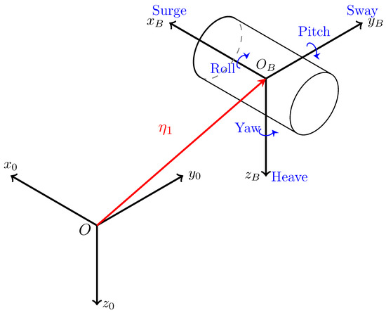
Figure 1.
Generic framework.
2.2. Kinematic Model
The position of the vehicle is given by the coordinates of the center of the mobile frame in . Let us define the position and orientation vector with the position of in and the orientation of with respect to represented with the Euler Roll–Pitch–Yaw angles convention. Note that the Euler angle representation introduces a singularity in . This singularity is of no consequence in most applications, but, for the few cases in which such a configuration could be reached, a non-singular description of the vehicle’s orientation such as quaternions can be used [16]. Nonetheless, such descriptions come at the cost of an additional parameter.
It is useful to introduce here the error representation chosen in this work. Error vectors will be denoted with i the name of the considered variable and always calculated as the difference between the desired and actual values of a variable. As an example, the position and orientation error vector is given as , where is the desired value of . It is also worth noting that the signs of the equations drawn from the references are adapted to follow this convention unless the opposite is specified.
To complete the definition of , let us introduce the velocity vector of the vehicle expressed in with respect to : , where is the vector of linear velocities, and is the vector of angular velocities.
The kinematic model of the vehicle is then given by the equation:
where is the first time derivative of vector , and is defined in this representation as [1]:
where being the rotation matrix of angle around axis . Additional definitions of can be found in [1,16,18] for the quaternion representation.
Some control methods presented later in this work require the definition of a tracking point E. The tracking point is the point of following the task. In some applications, the tracking point could be the focal point of a camera or the grasping point of a manipulator. Depending on the application, the tracking point could be either fixed or moving in . In this work, E is taken as a fixed point of coordinates in . Therefore, a solid kinematics law gives the linear velocities of E and angular velocities of the vehicle expressed in w.r.t. as :
with
2.3. Dynamic Model
Dynamic modeling of marine craft has been widely studied over the years, and many formulations exist with different levels of accuracy. In this work, the most common formulation of the model in the control community is used even if it is not the most accurate one from a hydrodynamics point of view. It is the one generally used in underwater robotics. In this context, hydrodynamic inaccuracies are seen as perturbations that will be rejected, in practice, by robust control of the craft. The dynamic model of the system in the marine environment is given by [16,19]
where is the generalized vector of propulsive forces and moments, is the matrix of mass, inertia and added mass, is the matrix of Coriolis and centripetal terms including hydrodynamic effects, is the damping matrix, and is the vector of gravitational forces and moments.
In (5), the hydrodynamic effects are linearly superposed to the rigid mass effects. The mass and Coriolis matrices are therefore defined as:
Matrices and refer to the mass effects of the rigid body while and are the hydrodynamic effects applied to the vehicle and called added mass effects. The interested reader can refer to [18,19,20,21] for more details about added mass coefficients, matrices structures for different vehicles and hull shapes as well as calculation and approximation methods for those coefficients.
2.4. Actuation Vector and Propulsive Configuration
The actuation vector in (5) is the vector of generalized forces and moments generated by the vehicle’s propulsion expressed in . The wrench is defined as:
with X, Y and Z the propulsion forces on axis , and , respectively, and K, M and N the moments around , and , respectively.
The thrusts produced by each thrusters of the vehicle or, in the case of reconfigurable thrusters, produced by equivalent stationary virtual thrusters are summed up in the vector of forces , where each row is the propulsion force of one thruster. The vector is calculated as:
where is the Thruster Configuration Matrix (TCM) detailed in [22,23], and is a vector containing the propulsive thrusts. Matrix defines the propulsive configuration of the vehicle. As an example, we consider an underwater vehicle equipped with 4-fixed thrusters: and longitudinal at the stern and and vertical in the middle of the hull. We call this configuration the “RSM”robot, and it is displayed in Figure 2. The TCM matrix of the RSM propulsive configuration is:
where is the coordinate of thruster i on the axis of .
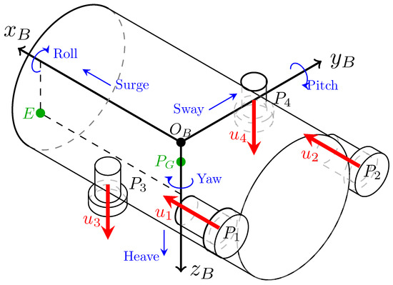
Figure 2.
Propulsive configuration of the RSM robot.
Because of the rows of zeros in the TCM matrix (8), the vector of propulsive forces and moments in for a vehicle such as the RSM robot will be of shape:
Therefore, the RSM robot is an example of an underactuated underwater vehicle for a 6-DOF task. The propulsive configuration cannot produce any force on the axis or moment around the axis.
In the case of fixed thrusters associated with rudders, the forces and moments generated by the rudder can be expressed as a function of the rudder angle and surge thrust as in [24], and a similar representation can be found.
3. Consequences of Underactuation on a Controlled System
In this study, it seems appropriate to relate the definition of underactuation to the task the vehicle is evaluated on. In fact, it is common practice [5,7] to consider a subspace of the six-dimensional space reduced to the degrees of freedom (DOF) required in the task. It is therefore mandatory to evaluate whether or not the system is completely actuated in this subspace. Thus, two parameters are considered when evaluating the actuation of a system: the number of actuated degrees of freedom of the system relatively to the number of degrees of freedom of the task and the coherence between these two sets of DOF. The number of independent degrees of freedom constrained by the task will often be referred to as task requirements in this work. For the first parameter, it is commonly known that a system which has fewer actuated degrees of freedom than the requirements of the task is underactuated. However, even if the system has as many actuated degrees of freedom as the task requires, the two sets of DOF may not match. In such a case, a problem like trajectory tracking becomes non-trivial and new mechanisms must be introduced in the guidance or control of the vehicle to make the best use of the actuated degrees of freedom to perform the task. Thus, in this case, the vehicle can also be considered underactuated. One way of seeing this case of poorly actuated vehicles is to consider the subspace of the required DOF of the task. In this subspace, such a vehicle would clearly appear underactuated. As will be seen later in this work, most traditional boats can be considered underactuated when it comes to reaching fixed waypoints; in addition, most glider submarines are underactuated when tracking a 3D trajectory.
The definition of the underactuated vehicle used in this work is the following:
Definition 1
(underactuated vehicle). A vehicle is considered underactuated if either:
- The vehicle has fewer actuated degrees of freedom than the task requirements;
- The vehicle has as many degrees of freedom as the task requires, but some of them are not in the subspace defined by the task requirements.
This definition of underactuation involves the fact that underactuated vehicles are not always controllable in the task subspace making the control problem non-trivial. While controllability criteria are hardly defined for nonlinear systems, differential flatness introduced in Section 7 is often raised as a good candidate.
As will be seen in this work, many methods exist to exploit the actuated degrees of freedom of an underactuated vehicle at best and especially when they do not match with the task. Although they are all different and complex, all the methods make use of a simple mechanism referred to in this work as the compensation of one or a few non-actuated DOF with another actuated one or ones. This is the most intuitive way to cope for the lack of actuation over a degree of freedom, and it is in used in most terrestrial and marine vehicles autonomous or not to this date.
A very quick generic example allows for getting a grasp of the idea of compensation and the notion of diagonal and non-diagonal problems. Let us consider a three-dimensional problem with state and input . In the most basic case (fully actuated and decoupled), a simplified input–output representation of the close-loop system can be given as
where are functions of the state and its first derivatives and a certain number of control parameters. The variables represent the error between and the desired value on this axis . In this first case, each control input is built upon the corresponding error signal in a one-to-one relationship, and the input–output matrix is diagonal. In such a case, a simple proportional gain could do as the function. Now, let us introduce underactuation in this simple system. One way of introducing a non-actuated degree of freedom in such a system is to consider that, whatever the required output value, the non-actuated input is always equal to 0. If the second degree of freedom is not actuated, the system becomes:
Comparing (10) and (11), it appears clearly that the values of and will be of no consequence over the input . This would lead to a parallel convergence where the errors and could converge to 0, but the error would be ignored. In this system, underactuation really is a problem only if the task is composed of the three DOF or of the first and second but not the third. If the task requires three independent DOFs, then the system is underactuated and there is no solution to control the three DOF at the same time. However, in a case where the task is composed of the first and second DOF but not the third, the third control input could be used to compensate for the lack of actuation on the second. In such a case, the subspace defined by the requirements of the task would be:
In the subspace defined in (12), the reduced system appears underactuated.
Then, to take into account, a new input–output matrix can be designed in the complete space as:
In the case (13), the error signal is used in the calculation of the input . This example shows compensation of the lack of actuation over with . Note that, for this compensation phenomenon to happen and actually have an incidence on , and cannot be orthogonal forces or a force and a moment around the same axis. Most of the time, and notably with autonomous vehicles and marine craft, is a linear force, and is chosen as a moment around any axis orthogonal to . With a well-chosen , most often based on the system model, convergence of to 0 can be attained. However, this comes at a cost since it is now that is ignored. It is the designer’s choice to decide which of the degrees of freedom of the system must be prioritized or which error can be left non-zero without risking the application.
4. Line of Sight Guidance
The Line Of Sight guidance technique (LOS) [3,25,26,27] is the most intuitive guidance method for most marine vehicles both on the surface and underwater. The basic idea is rather simple: when piloting a typical boat, the easiest and fastest way to reach a distant waypoint is to point the boat towards the waypoint and sail straight forward. Once the waypoint or its neighborhood is reached, the boat is pointed towards the next one and so on.
While being quite simple, the idea behind LOS guidance hides interesting concepts. Inherited from traditional naval techniques, LOS guidance has initially been designed for autonomous boats. Such vehicles are typically underactuated in the horizontal plane. Only surge and yaw are actuated on most surface vehicles and sway is passively stabilized by the hull shape making trajectory tracking in the horizontal plane non-trivial. These vehicles will be referred to as -boats or -vessels in the following. There are three main actuation topologies for -boats: a fixed rear longitudinal thruster and a rudder, a single reconfigurable rear thruster or two fixed rear thrusters. These three topologies allow for generating both a surge force and a yaw moment. Few differences exist between the three possible topologies of a -boat and notably when it comes to decoupling of the surge and yaw speeds. While not being treated in this work, the possible couplings between surge and yaw actuation may lead to different performances for a given control or guidance method. The most common task LOS guidance is applied to its reaching waypoints where the waypoints are a set of fixed points of the horizontal plane. Waypoint reaching has later been extended to trajectory tracking considering either a mobile waypoint or a set of waypoints close to each other associated with a propagation rule.
A very simple LOS guidance is given in Figure 3 and in Section 6.5 of [1]. Here, a new heading reference is calculated based upon the position error between the vehicle and the tracked waypoint calculated in the inertial frame. Proportional control allows for tracking of the said heading reference. The surge speed is set to a constant. It could be controlled with another PI-based controller as well. Once the neighborhood of the current waypoint is reached, the next one is targeted. This simple LOS guidance principle does not take the model of the vehicle into account nor does it compensate for any external disturbances. Intuitively, the heading reference would be calculated as:
In (14), the function is used instead of the classical function to avoid singularities. This expression is commonly used in numerical calculation; it extends the definition of to the complete complex plane. The function is defined on the four quadrants of the complex plane as:
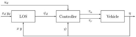
Figure 3.
Block diagram of a simple Line Of Sight Guidance control. The Controller block represents any control function capable of calculating the surge and yaw controls and from the desired and current states.
A more advanced control based on LOS guidance is given in [2]. In this work, LOS guidance algorithms provide desired heading and its first and second order derivatives. The nonlinearities of the model are taken into account and linearizing terms are added in the controller in a hybrid feedback and feedforward fashion (see Section 5 for more details on linearizing controllers). The two controller equations can be expressed as:
where are coefficients of the mass matrix, are coefficients of the Coriolis and damping matrix, , and c are control gains. The yaw speed control is calculated as an intermediate command variable in the kinematic controller (15d). In the controller given by (15a), the heading references , and are outputs of an extended LOS guidance algorithm similar to (14).
LOS guidance can also be applied in the underwater three-dimensional case as displayed in [3]. Underwater, LOS guidance is mainly used for vehicles actuated in surge, pitch and yaw (called -vessels in the following). For -vessels, pitch and yaw are generally used to cope for the lack of sway and heave actuation therefore allowing tracking of waypoints or trajectories. The same principle as for 2D LOS guidance is applied, and the vehicle is pointed towards the tracked point and is propelled forward. As shown in [3], 3D LOS guidance involves an additional angle: the elevation. As in the 2D case, the heading and elevation angles given by LOS guidance can be used as references in the yaw and pitch controllers respectively.
The work in [3] provides three assumptions for convergence of the LOS guidance and also makes use of two additional control parameters called look-ahead distances. In simple terms, when look-ahead distances are used, the ship is not pointed towards the target itself but towards a fictional point slightly further away on the trajectory. Look-ahead distances allow a smoother trajectory convergence and can be tuned relatively to the application and system. This work also introduces a path frame centered on the tracked point p. Conditions upon the evolution of point p are given in this work to ensure convergence in the form of an equation giving the evolution speed of point p relatively to the desired speed of the vehicle. The tracking errors used for the calculation of the reference elevation and heading angles of the LOS algorithm are calculated in frame .
In [25], the same authors apply the principle of 3D LOS guidance to a -ship and build a complete controller upon this principle. As seen before, the LOS angles are used as references in the pitch and yaw controllers. This work also gives a lead towards unification of fully-actuated and underactuated controllers, taking into account the fact that some actuated DOF may be considered non-actuated in certain speed ranges. In addition, Ref. [26] gives experimental results of a similar control method in the case of an underwater vehicle tracking a predefined fixed-depth path close to the surface.
The LOS guidance principles described up to this point do not take external disturbances like marine current, wind or waves into account. In fact, traditional LOS guidance does not ensure theoretical convergence in the presence of external disturbances. To cope for such disturbances, Ref. [27] proposes adding a new term in the traditional LOS heading angle calculation in the case of a -vessel. This new term, denoted as , behaves like the integral term of a PI controller would, and it cancels possible steady state error due to persistent external disturbances. Though is not calculated as the integral of y, its propagation function will be chosen to allow convergence of the closed-loop system. Therefore, will be referred to as a pseudo-integral term. Considering , the modified LOS heading angle can be expressed as:
In (16), is a new control parameter acting as an integral gain, and is the look-ahead distance. As is always strictly positive, RHS of Equation (16) is always defined, and the value of is always in . For a complete four quadrants output, one may use the function instead.
Equation (16b) gives the propagation rate of the integral term . The first order derivative of the pseudo-integral term is conveniently chosen to allow convergence of the closed-loop system.
In [27], the tracked trajectory is a straight-line path defined in by . Therefore, the position of the vehicle y used in (16) could be replaced by the cross-track error for different trajectories. Nonetheless, having the integral term in (16) allows the vehicle to move along the path with a non-zero relative heading angle in case of external disturbances. An adaptive yaw controller is then given and convergence is proven in the presence of external disturbances.
The work presented in [28,29] provides a generalization of the integral LOS guidance in 3D in the presence of sea currents. In the former, the addition of an integral term in the elevation angle calculation allows for compensation of vertical oceanic current in the case of a horizontal trajectory tracking problem for a -ship while, in the latter, both elevation and heading angles are given with an integral term therefore allowing robustness to any irrotational current. The example in [29] is interested in tracking the x-axis line defined by . The enhanced heading angle in [29] is similar to (16), and the elevation angle is built the same way but with the z tracking error:
In [24,30], a slightly different approach of LOS guidance is proposed. Here, the calculation of the desired LOS heading angle is based upon the cross-track error. The cross-track error kinematics is given by:
where is the velocity of the ship, is the trajectory heading angle, and is the slide-slip angle of the vehicle. The variable s can be considered as a curvilinear abscissa whom propagation rule is given in [24]. More details about the path frame used here can be found in the references. Thus, the cross-track error kinematics (18a) can be seen as a new tracking problem of input and output , where is the course angle. A new formulation of the desired LOS heading angle is given to stabilize the cross-track error towards the equilibrium point ; the so-called proportional LOS guidance:
It is worth noting that [24] proposes an alternative representation of the problem. A pivot point is introduced and is chosen as the point of the vehicle where the local sway velocity is zero. The pivot point is considered as the new tracking point. A new definition of the cross-track error and of the tracking problem in general is given in this point. The proportional LOS guidance is demonstrated as being uniform semiglobal exponential stable (USGES) for the -boat. Surge and Yaw controllers are given in this case based on the cross-track error. In addition to minimizing the cross-track error, the work of [30] also includes minimization of the along-track error with a surge speed controller taking both cross-track and along-track errors into account.
LOS guidance has received a lot of attention over the years and many more references could be added in this work. The method has been used in different applications such as waypoint tracking control in [31], studies on the optimization of the look-ahead distance choice have been conducted as in [30], and LOS guidance has been applied to smooth transitions between fully-actuated and underactuated configurations in [32] and, up to this date, more work is conducted on the application of LOS guidance to different marine craft [33,34].
Overall, LOS guidance can be considered as the go-to method for automation of -vessels in surface or planar applications or -ships for underwater applications. However, as can be seen here, LOS guidance is not suited for applications where orientation of the vehicle is controlled. In fact, LOS is one of the methods using a rotational DOF to compensate the lack of actuation on a translation. In the -ship case, yaw moment is used to compensate for the lack of sway. However, the difference between LOS guidance and the other compensation methods given later in this work is that, with LOS guidance, the compensation occurs at the guidance level while, in the following, it happens mostly at the controller level. Using two translation errors or two translation speeds in the calculation of a reference for a rotational DOF makes the controller on the latter a function of either of these translation signals. This kind of manipulation is useful for underactuated systems since it allows for going beyond the traditional one to one diagonal controller systems where control over a DOF is calculated upon the error on this same DOF. Other methods of this kind are presented in the following.
5. Model-Based Linearization and PID Control
The very early works in (static state) feedback linearization can be found in W. Korobov [35] and R.W. Brockett [36]. The necessary and sufficient conditions of feedback linearization have been obtained by B. Jakubczyk and W. Respondek [37]; see the works of R. Su and A. J. van der Schaft [38,39] for the general extension to the nonlinear case. Refer to D. Claude [40] for a survey. The problem of dynamic feedback linearization has been later addressed by B. Charlet, J. Lévine and R. Marino [41]. See also the books [42,43,44] for more references. Recall that the problem of dynamic state feedback linearization is still open. The input–output linearization problem has been first addressed in [45] and completely solved in an algebraic setting in [46].
Proportional Integral Derivative (PID) control is the most well-known and widely spread control technique among autonomous systems. However, when it comes to marine craft and nonlinear systems in general, PID control itself may not be enough to cancel the state error in trajectory tracking tasks. Additional linearizing mechanisms must be associated with PID control when working with nonlinear systems such as autonomous boats or underwater vehicles. This section demonstrates the use of PID control and these additional strategies in the case of marine craft. The main advantage of adding linearizing terms to the control law is to create a linear closed-loop system by canceling the nonlinearities of the model, whereas a PID controller alone applied to a nonlinear system would be particularly difficult to tune and concluding on the convergence and stability of the closed-loop system would not be possible.
This section displays an example of PID-based controllers both in the fully actuated case and in the underactuated case. Note that, in the fully actuated case, the common use of diagonal gain matrices create a 1-to-1 relationship between input and output only tempered by non-diagonal linearizing terms. In the underactuated case, on the other hand, additional non-diagonal mechanisms allow for creating the compensation behaviors introduced earlier in this work.
This section mainly focuses on model-based linearization methods but model-free, adaptive controllers also exist and some examples of such controllers can also be found in [1,5,47].
In fact, linearizing model-based controllers can be broken down into three classes. The first type is State Feedback Linearization, often referred to as Exact Linearization [1,47]. Here, components of the model evaluated at the current state of the system are used in the controller in order to theoretically exactly cancel the nonlinearities in the closed-loop system. Practically, some nonlinear terms may appear in the closed loop system depending on the experimental conditions. Nonetheless, the main advantage of using exact linearization is to turn the original nonlinear control problem into a linear closed-loop system tuning problem in which conventional PID setting methods as pole placement or linear quadratic regulation can be used.
The second class of linearizing model-based controllers can be referred to as Feedforward Linearization or Non-exact Linearization in opposition to the first one [1,4]. Here, the model parameters added to the controller are evaluated at the desired state or at a virtual reference. Therefore, as long as the current state is different to the desired state or the reference used in the feedforward terms, the nonlinear terms of the system are not exactly canceled in the closed-loop system. The resulting state error dynamics can therefore remain nonlinear. In this second case, conventional tuning methods are therefore more difficult to set up on the resulting closed-loop system. As will be detailed later in this section, the idea of using a virtual reference in the controller can be apprehended as having two nested control loops or two stages. As a simple example, the virtual reference in the case of marine craft would be a virtual speed vector built itself as a controller assuring convergence of the position of the vehicle towards the trajectory. Roughly speaking, the outer loop generates an effort control vector ensuring convergence of the vehicle’s speed towards the virtual reference. This virtual reference is calculated as a speed controller output assuring convergence of the position towards the trajectory. Figure 4 displays simple block diagrams of feedback and feedforward linearizing controllers.
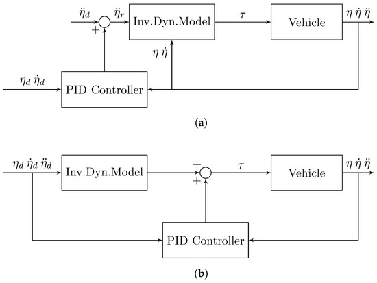
Figure 4.
Comparison of the feedback and feedforward linearizing controllers. (a) block diagram of a feedback linearizing controller; (b) block diagram of a feedforward linearizing controller.
The third class of linearizing model-based controllers is hybrid [5,47]. In these controllers, both feedback and feedforward terms are used to cancel only some of the nonlinearities of the system. Such controllers can be used to bring few “well-behaving” nonlinear terms in the closed-loop system, therefore enhancing the overall performances. Outside of the marine context and with other types of controllers, details about these nonlinearities of the closed-loop system and their interest can be found in [48]. Some of the examples introduced in this section allow for comparing hybrid linearizing controllers using different amounts of nonlinear terms.
5.1. Generic Example of State Feedback Linearization
A generic example of state feedback linearization can be found in [44]. As one may have noticed already, the dynamic model (5) can be given in the companion form.
Let us introduce a nonlinear system of state x and input u. For simplicity, the system used here is of scalar state and input:
The functions and are known nonlinear functions of the state x. Assuming that is non-singular and, using the inverse of Equation (20), it is possible to build a command vector u such as:
In this equation, is a positive gain and are the desired state and first order derivative of the desired state. The closed-loop system is therefore given by:
Equation (22) shows that the feedback linearizing controller given in (21) leads to a linear state error differential equation, namely , whose all solution asymptotically converges to 0. In this example, exact feedback linearization is used since the actual values of the state and the model matrices evaluated at the current state are used in the control to cancel the nonlinearities of the model and lead to a linear closed-loop dynamics. Development of the general case, with a state of dimension n and a control of dimension m, is left to the reader.
Obviously, such linearizing controllers are not only used with marine vehicles. They can be applied to many nonlinear systems as in [49,50]. Linearizing controllers are applied to a generic dynamic system in the former and to a manipulator arm in the latter. These two references refer to the methods used as the Computed torque. Although it is very close to the linearization methods used in the following examples, the term “computed torque” is rarely used when working with marine craft.
5.2. PID Control and Model-Based Linearization in the Fully Actuated Case
5.2.1. Feedforward Linearizing Controllers
A first example of a non-exact linearizing controller can be found in [4]. In this work, the model is considered in the inertial frame and an expression of the model matrices expressed in the inertial frame can be found in the reference. The modified matrices are indicated with a ∗. The controller is given by the set of equations:
In Equation (23), the orientation of the vehicle is represented in quaternions as part of the vector , and is the state error. The matrices , , and are strictly definite positive gain matrices that are set to the identity in this work but could be tuned for better performances. The reference [4] specifies that removing the integral term by setting to 0 does not disturb the global convergence of the method.
In the control law (23), is built as a conventional PID controller outputting an acceleration vector and is a virtual speed reference as explained at the beginning of this section. This reference can be seen as a kinematic controller assuring convergence of the position of the vehicle towards the trajectory. It is interesting to note that, when the state error tends to zero, the virtual speed reference tends to the desired speed in the inertial frame multiplied by a control parameter .
Removing the integral terms of the controller, the closed-loop error system can be expressed in the inertial frame as:
Because of the “non-exact” linearization used in this example, the closed-loop dynamics (24) is nonlinear. However, the reference [4] states that the system is globally asymptotically convergent.
Similar examples of nonlinear PD controllers for trajectory tracking are demonstrated in Sections 7 and 14 of [1]. Here, the control laws are given in the mobile frame as:
Again, (and thus ) can be considered as the virtual speed reference used in the feedforward part of the control law . Because the nonlinear terms of the model are evaluated at that reference instead of the actual state of the system, nonlinearities will remain in the closed-loop system. However, it should be noted that, once the position error is canceled (), the speed reference is equal to the desired speed . Therefore, when the vehicle converges towards the desired state, the controller behaves like a feedforward controller, introducing nonlinear terms in the closed-loop. As will be seen later, these nonlinear error terms in the closed-loop system may be beneficial for the overall behavior of the system.
As with the previous example, Equation (25c) can be seen as a kinematic stage ensuring convergence of the vehicle position towards the trajectory, and (25a) can be seen as the dynamical stage dealing with convergence of the speed of the vehicle towards the virtual reference . However, this separation of the two levels is made difficult because of the two additional position and speed control terms in the dynamic stage. A simple block diagram of a generic two-staged controller is displayed in Figure 5. On this diagram, the outer stage uses the inverse kinematic model to calculate a speed control ensuring convergence of the position of the vehicle towards the trajectory, and the inner stage uses the inverse dynamic model to calculate a command vector ensuring convergence of the speed of the vehicle towards the speed command.
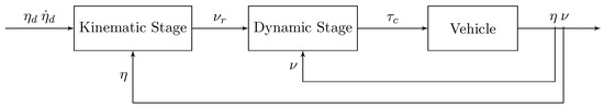
Figure 5.
Simple block diagram of a two-staged controller.
5.2.2. Feedback Linearizing Controllers
There is a second example of a PID-based linearizing controller in [1] (in Sections 7 and 14), but this one uses exact linearization. The closed-loop system obtained when applying the controller is linear. The control law is given by:
In (26), the acceleration reference is built as a typical PID controller associated with the acceleration feedforward term . This control law is very close to the generic example given earlier in this section. It is clear that applying the control law (26) leads to a linear closed-loop system dynamics. In fact, because they are evaluated at the actual state of the system, the nonlinearities of the model are exactly canceled by the control law. The closed-loop system is now:
The exact feedback linearization used in this example allows global exponential convergence of both the speed and position of the vehicle. This example also highlights another advantage of the exact linearization, which is that it allows using traditional gain tuning methods on the closed-loop system such as pole placement or LQ regulation.
5.2.3. Hybrid Linearizing Controllers
Examples of hybrid linearizing controllers can be found in [5]. This work proposes and compares a set of controllers using either a hybrid linearization with both feedforward and feedback terms, fully non-exact linearization or adaptive structures. The model-based controllers introduced in [5] show interesting results. First, a conventional PD controller that does not rely on the model, is given as a baseline for comparison. The PD control law is given as:
As said in the introduction of this section, a simple PD controller is unlikely to show good performances when used to control a marine craft on complex trajectory tracking tasks. However, it is worth mentioning here because it can be a first step towards an autonomous vehicle and give results on simple set point tasks.
Note that, in [5], the system is represented with a decoupled model. All non-diagonal terms are neglected and notably the non-diagonal added masses and Coriolis and centripetal terms. Therefore, most of the nonlinearities of the model are neglected. The model can therefore be considered as six independent nonlinear subsystems, one per degree of freedom. In addition, the linear and quadratic terms are broken apart and regrouped in two different matrices, respectively, and . The first control law is given as:
The control law (29) is hybrid in the sense that it mixes feedforward and feedback terms. The control law can be broken down into three parts. First, one finds a traditional PD controller similar to the baseline PD control law (28): . Matrices and are usual gain matrices. Then, the linear part of the reduced model is added and evaluated at the desired state, that is: . Finally, the nonlinear terms of quadratic damping and gravity, buoyancy and disturbance effects are added and evaluated at the actual state: . This last part is exactly canceling the nonlinear part of the system.
Now, let us introduce the second control law of [5] for the sake of comparing the closed-loop systems they both lead to. This second control law is mostly similar to the first one, but this time feedforward is used in the quadratic damping. The second control law is then:
Note that exact feedback values of the nonlinear gravity, buoyancy and disturbance term are used anyway.
The two closed-loop systems are then given by:
Because of the slightly different constructions of the two control laws, the second closed-loop system (31b) shows an additional quadratic speed error term. Both control laws are exponentially convergent in both speeds and positions. Due to the system simplification, the differences in behavior are very small in this example, but a small improvement on the convergence time can be observed with the second control law.
Another similar comparison is made in [47]. In this work, the system model is complete, and two control laws are produced. The first one is a completely exactly feedback-linearizing controller while the second one uses feedforward terms in the damping term. The two control laws are given by:
Note that, in these two control laws, the PD controller terms are used as part of the reference acceleration term instead of being just linearly added to the linearizing terms. This method essentially allows for simplifying the mass matrix in the closed-loop system equations, making them independent from the mass matrix and avoids introducing nonlinear error terms in the closed-loop system. The two closed-loop systems are given as:
In this work, the addition of quadratic speed error terms in the second closed-loop system leads to better trajectory tracking performances. It appears that the nonlinear damping term of this second solution behaves well and enhances the performances.
This section presents some linearization methods used with PID control in the context of fully-actuated marine craft. Figure 4 shows the difference between a completely exact linearization and a completely non-exact one. Of course, more combinations of feedforward and feedback terms could be used but are not treated here. Nonetheless, this section shows that the knowledge of the model can be used to simplify the nonlinear system, lead to a linear or partially linear closed-loop system and therefore allow using a conventional tuning method for the PID like pole placement or LQR1. Of course, similarities with the methods presented in this section will be found in the following sections because these linearization techniques are also used with other classes of controllers.
The interested reader is also referred to [5,47,52,53,54,55], for example, of PID-based controllers using adaptive structures for linearization. Although adaptive controllers are not detailed in this work, they are worth mentioning. Indeed, the model-based linearization methods introduced in this section require a precise estimation of the model parameters to perform at best. Adaptive methods on the other hand only require minimal model knowledge and are shown to perform as well as the model-based ones. The idea of these adaptive structure is to consider a set of variable gains and find propagation functions for these gains such that they progressively converge towards the real values of the model parameters. Then, the adaptive terms can be used to linearize the model and create linear closed-loop systems.
5.3. PID Control and Model-Based Linearization in the Underactuated Case
In the underactuated case, the linearization and PID control examples introduced in the above are not sufficient. Indeed, following the example of Section 3, the PID-based control laws introduced before would neglect some degrees of freedom in the underactuated case because they are diagonal. In order to take the non actuated degrees of freedom into account, the examples introduced in this section use either a non-diagonal space reduction or a non-diagonal, kinematic couplings-based gain matrix in the control law. In both cases, the kinematic couplings of the model are used as a guidance principle in a similar fashion as LOS guidance. Thanks to kinematic couplings, rotational speeds are calculated in the control law to compensate for the lack of actuation on a non actuated translation.
The first mechanism used in addition to model-based linearization and PID control is asymmetrical Space reduction. Space reduction is a method consisting of reducing the spatial dimension of the system and considering only some of the degrees of freedom of the system. It is common practice when it comes to dealing with underactuated systems and especially for a system where one or more degrees of freedom are both non-actuated and naturally mechanically stable. As an example, it is common to neglect the roll motion of a torpedo shape vehicle if the restoring moment in roll is considered strong enough to keep an almost zero-roll angle during all the application time or if this DOF has no meaningful impact on the mission. In such a case, the problem can be reduced to a five-DOF problem. However, when it comes to vehicles and applications whose degrees of freedom do not match, space reduction gets more complicated but offers new possibilities. In the following examples, space reduction can be considered asymmetrical because the method considers different degrees of freedom at the tracking point and at the center of vehicle, therefore introducing some non-diagonal terms in the control law.
As a first example, Ref. [56] proposes a solution to the 3-DOF position tracking problem applied to a generic -craft in which space reduction is used as a guidance mechanism. First, let us define a tracking point E fixed in the mobile frame . Using a E as a tracking point means that E is required to follow the trajectory and no longer the center of the mobile frame , as it was in the previous sections. This tracking point can be chosen anywhere in the mobile frame and usually represents either the bow of the ship, the focal point of a sensor or an end effector. In [56], E is chosen on the axis of the mobile frame. Using (1) and (3), the system kinematics can be rewritten as:
with the velocity vector of point E in , and the transformation matrix given in (4) with and .
In [56], a reduced version of Equation (34) is then produced with reduced matrices and vectors. Because and are expressed at point E, they are reduced following the DOF required in the application so the three last rows and columns are discarded. On the other hand, is expressed in point and is therefore reduced following the actuated DOF of the ship so the second, third and fifth rows are discarded. In addition, because the transformation matrix is used to move from E to , the rows are reduced following the DOF required in the application while the columns are reduced following the actuated DOF. Therefore, the three last rows and columns 2, 3 and 5 are discarded in . The reduced kinematic model is then given as:
The reduction of the dynamic equation is more straightforward since all the matrices and vectors are expressed in point and reduced in the same way, keeping the first, fifth and sixth rows and columns.
The control law presented in [56] is composed of two stages, kinematic and dynamic ones. The kinematic stage is a proportional controller with an anticipation term based on the position error calculated in . The equation of the kinematic stage is given in by:
with a definite positive gain matrix and a drift vector accounting for the neglected translation motions and current speeds. Note that stands for a control speed at the tracking point E supposed to ensure convergence of the position of the tracking point towards the trajectory. All the vectors and matrices of Equation (36) are reduced following the steps presented before, but the index r is omitted for clarity.
The dynamic stage is built like a common computed torque control in the reduced space. One obtains:
where is the output velocity vector of the kinematic stage, and is a vector containing some terms discarded during the space reduction and considered as external disturbances. Equation (37) is expressed following the space reduction presented before.
Therefore, looking at (35) and (36), it appears clearly that the pitch and yaw control speeds at the output of the kinematic stage and are functions of the sway and heave control speeds in point E, and , respectively. Therefore, the pitch and yaw components of are themselves calculated out of the lateral and vertical motions required in point E. This behavior is created by the asymmetrical space reduction and notably the introduction of non-diagonal terms in the reduced transformation matrix .
The method developed in [56] has been extended to different propulsive topologies and applications in [23,57]. In [57], the space reduction method is applied to two different underwater vehicles. The first one is the RSM robot displayed in Figure 2. It is equipped with four fixed thrusters generating surge and heave forces as well as roll and yaw moments. The second vehicle is equipped with a stern vector thruster generating surge force as well as pitch and yaw moments which is shown equivalent to three fixed stern thrusters aligned to the body-fixed axes. This second vehicle will be called the 1D3-Robot in this work and is displayed in Figure 6. Both vehicles are evaluated on the same 4-DOF task defined by the position vector in and the heading angle . Therefore, both vehicles are underactuated relatively to the task. The first vehicle has the correct number of DOF but lacks sway actuation and is actuated in roll, which is not required for the task at hand. The second vehicle has three actuated DOF, thus making it unable to completely meet the task. For this second vehicle, the task is reduced to the three positions only.
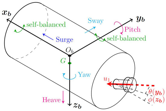
Figure 6.
Propulsive configuration of the 1D3-Robot. It is equipped with one 3-DOF reconfigurable thruster at the stern.
Then, the space reductions in [57] are different from the one introduced in [56]. For the first vehicle, the vector and matrices expressed in are reduced discarding the second and fifth rows and columns, whereas the vectors and matrices expressed in E are reduced discarding the fourth and fifth rows and columns. For the second vehicle, only three DOF of the vehicle are actuated. The vectors and matrices in E are then reduced, keeping only the three first rows and columns while those expressed in are reduced keeping the first, fourth and fifth rows and columns. The shape of the vectors and matrices for both vehicles are described in detail in [57].
Partial convergence of the method is demonstrated in [23] for the first 4-DOF vehicle. The compensation mechanism allows sway tracking in E but at the cost of yaw. Nonetheless, the heading of the vehicle is kept stable thanks to hydrodynamic restoring moments and stays very close to the task requirements.
Overall, in the examples presented above, the reduced translation matrix behaves like a non-diagonal gain matrix making the speed command of one DOF in depending on the speed command in E on another DOF. As the previous solutions shown in this work, this method allows compensation of the lack of actuation over one degree of freedom with another. Preferably, a rotational DOF would be used to compensate the lack of a translation. However, one of the major issues of such methods is that reduced matrices lose some of their properties. Notably, the reduction of the might, in some cases, add new singularities to the system, making the matrix noninvertible for some orientations.
Similar behavior can be obtained without space reduction introducing a model-based non-diagonal gain matrix in the kinematic stage of the controller as displayed in [58] (only in French for now). In this example, the so-called Handy matrix is introduced in the kinematic stage of the control law to allow compensation of the non-actuated sway motion with yaw. This matrix is autonomously calculated by an algorithm provided in this work and is based on the kinematic couplings of the model. It allows for generating the yaw moment necessary to exactly create the sway speed in the tracking point E required to cancel the lateral error. The interest of this method is that it does not require reducing the space of the application which makes generalization easy.
6. Sliding Mode Control
After the famous book by I. Flügge-Lotz [59] on discontinuous control, the sliding regime control was essentially introduced by a few authors in the end of the 1950s [60,61,62,63,64]. These works were followed by those of Cypkin [65], Emelyanov [66] and Itkis [67]. Utkin introduced a notion, new for the time, of sliding control applied to mono-variable classical linear systems, by the use of discontinuous controls [68]. See also [69] for a survey. All of these ideas would not have been possible without the much more theoretical work of the Soviet mathematician Filippov in the 1960s concerning differential equations with a discontinuous right-hand side [70]. The books of Utkin [68] and Sira-Ramírez [71] give a good overview of this approach to discontinuous control which has gained popularity its simplicity and its applications in various fields of automation. Moreover, these techniques have led to industrial applications. The applications of SMC in robotics and AUV start with the works of J.J.E. Slotine: [6,72,73,74].
This section introduces the use of Sliding Mode Control for both fully-actuated and underactuated marine craft. SMC is widely used in both linear and nonlinear systems experiencing model uncertainties or external disturbances. SMC is known for its robustness [6] and for offering theoretical finite time convergence even in the presence of model approximations and external disturbances. Finite time convergence is made possible by the introduction of a sign function in the controller, but the use of the discontinuous sign function in SMC induces a new phenomenon called chattering. Chattering is a consequence of a discontinuity in the controller around the equilibrium point creating fast steep oscillations potentially damaging for the actuators. Chattering can be mitigated or completely avoided using different methods but at the cost of asymptotic convergence instead of finite time convergence. Many examples of successful application of SMC on surface vehicles and underwater craft can be found in the literature. This section presents some of them after briefly introducing the method on a generic simple example. This example is also used for introduction of the notations relative to SMC. The interested reader is referred to [9,44,75,76] for more information about SMC outside of the marine environment. Note that, when SMC is applied to nonlinear systems, similar techniques as in Section 5 are used to make the closed-loop system linear.
An example of basic SMC can be found in [44]. Let us recall the system used in the first example of Section 5, in the case of a n-order system, as:
The state of the system is defined as . Referring to the model introduced in Section 2, matrix can be seen as the inverse of a mass matrix and vector as the vector regrouping all other effects of force, notably the Coriolis and centripetal effects as well as damping. An additional vector of disturbances could be added in the system, but it is neglected in this example for the sake of simplicity. Finally, is the system input. In this example, and are considered known but further analysis in the case of approximated model matrices can be found in [6,44].
The idea behind SMC is to reduce the control problem to the lower-order problem of minimizing the distance between a point in state-space and a surface. The said sliding surface is in fact a state-space hypersurface2 representing the desired dynamics of the system. It appears in the literature that a confusion is often made between the actual sliding surface and the distance between the current state and the surface. When referring to the “sliding surface”, authors often use the equation of zero distance to the surface. In fact, the sliding surface itself is the set of desired states represented in state space, and it can be defined by the ensemble of system states where the distance to the surface is zero. In this work, the distance representation will often be used keeping in mind that the sliding surface is, in fact, properly defined as the states where this distance is zero. This choice is the most common in the literature because the distance to the surface is a function of the state error which is used to close the loop in the controllers.
As will be seen later, the question of defining the sliding surface has been widely studied in the literature, but a basic definition of such a surface associated with the distance measure is given by:
To match with the model used in this work, the example is presented with and therefore . The quantity is a design parameter representing the slope of the surface in state space. It can be tuned for better performances or relative to the application. Equation (39) shows that, in trajectory tracking applications, the sliding surface moves with the reference. One can also observe that the equilibrium point , is contained in the surface . Therefore, the control problem becomes a problem of minimization of the distance . Once the surface is reached, the sliding motion drives the system on the surface towards the equilibrium point , giving its name to the method.
The design of the command vector relatively to the sliding surface is based on the Lyapunov theory. Let us define the following Lyapunov function candidate:
for which ones obviously have and for . The Lie derivative of V is given by:
and the stability criteria therefore leads to:
Equation (42) is referred to as the sliding condition. One of the solutions of the sliding condition is given by:
where is a control gain to be tuned later. Using , the model Equation (38) can be combined to the sliding condition (43) to give an expression of the control vector :
One could rewrite Equation (44) as:
where the so-called equivalent term is in fact a feedback linearizing term of reference (see Section 5), and is the switching term assuring convergence towards the sliding surface. In the case of an approximated model, would be based on the model matrices approximation and would only compensate the known parts of the model matrices.
Note that, in a real application, the simple controller (44) is likely to create chattering as the switching of the sign function would not be instantaneous. The following examples propose alternative switching functions reducing or avoiding chattering.
6.1. Sliding Mode Control for Fully-Actuated Vehicles
The work of [6] gives a good example of SMC applied to fully-actuated marine craft, and the formulation is the same as in the example exposed before. The system has three actuated DOFs and is sent on a horizontal plane application composed of trajectories. In [6], the model is not entirely known a priori and estimated values of the model matrices are used in the controller. The model also includes approximated disturbances. All approximations are bounded, and this work shows that, when they are known, the estimation bounds can be used for the calculation of the gain parameter (noted in the reference) to ensure convergence. In addition, Ref. [6] displays the use of a different switching function based on a saturation function instead of a sign function. The saturation function shown in Figure 7 is better suited for real applications since it avoids the chattering phenomenon. Using the saturation function allows for creating some kind of boundary layer around the sliding surface where the switching effect is made continuous. The saturation function is defined as:
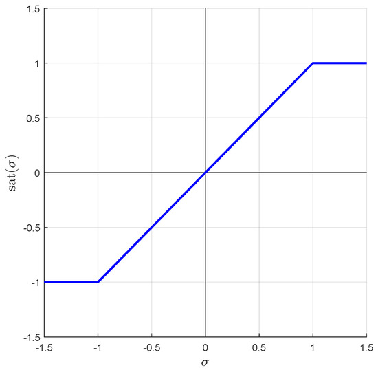
Figure 7.
The saturation function.
Using the saturation function (46), it appears clearly that, inside the boundary layer defined by , the nonlinear controller like (44) becomes very similar to the PID-based linearizing controllers introduced in Section 5. The controller becomes:
Therefore, the main drawback of using a continuous switching function such as the saturation function is that the convergence cannot be guarantied in finite time anymore. Nonetheless, Ref. [6] gives a method for calculation of the control gain, the slope of the surface and the boundary layer thickness based on the estimation of the model matrices, and shows very good tracking results.
The method is then used for the design of three decoupled controllers, one per actuated DOF. For each DOF, a sliding surface is defined as well as the different control parameters such as the boundary layer thickness or the switch control gain. The three sliding surfaces are given as:
One could observe that the surge and sway surfaces given by (48a) and (48b), respectively, are defined in terms of positions in the inertial frame and velocities in the body-fixed frame . While this could be fine for simple mono-axial applications, such a definition of the surge and sway sliding surfaces may be problematic when it comes to more complex trajectories. In this case, the trajectory tracking results show good performances.
The work of [7] is another good example of SMC following the same overall logic. Here, the vehicle is controlled only in the dive plane and is fully-actuated w.r.t. the task. In this work, the performances of four different controllers based on SMC are compared. The main difference between the four controllers is the model used in the equivalent part (see below Equation (51)). The first one uses a linearized model, the second one uses the nonlinear exact model, the third one uses an adaptive model, and the last one uses estimated states. The compliance and robustness of the SMC method allow such differences between controllers applied to the same system and is once again demonstrated by the results of this work.
The definition of the sliding surface is also slightly different in [7] since a first order linear surface, defined by , is used. Here, is a reduction of the state of the vehicle in the diving plane, is a vector of gains, and contains, in fact, three decoupled surfaces, one per DOF. The use of first order sliding surfaces allows for a simpler command vector and also enables the use of pole-placement techniques when tuning the parameters.
Another different definition of the set of sliding surfaces is given in [8]. As in [6], the sliding surfaces are defined in terms of the position errors in the inertial frame summed to speed errors in the moving frame. The set of sliding surfaces is given by:
where and being coefficient matrices are defined in . To take better account of the coupling effects between the DOF of the system, the sliding surfaces used here are defined over the full state space while, in the references presented before, they are often defined only on the output. For ease of understanding of the following equations, another expression of the vehicle model is given to match both the notation of Section 2 and the notation used in the reference:
The definition of the sliding surfaces (49) leads to a different expression of the control vector:
In (51), the estimates , and of the model function are used. A similar definition of the control vector could be given with the real values of the model functions if they were to be considered known. As for the usual definition of SMC given earlier in this section, the control vector can be broken down into three parts. compensates the estimates of the dynamic effects of the model, provides stabilization based on estimates of the positional elements in , and is the switching term driving the system to the sliding surfaces. This work uses the hyperbolic tangent function over the boundary layer of thickness as a switching function:
The hyperbolic tangent function is displayed in Figure 8 with . The hyperbolic tangent appears ideal since it is smooth around the equilibrium point but is still steep enough around the sliding surface to ensure fast switching and the sliding behavior.
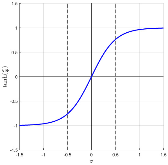
Figure 8.
The hyperbolic tangent function for .
Here, again, the structure of the control law is very similar to some controllers introduced in Section 5 and notably when the distance to the sliding surface is close to zero.
As for the saturation function seen before, using the hyperbolic tangent avoids chattering at the cost of a non-finite convergence time.
In order to set the values of and , the system is linearized. Doing so highlights that the first parameter matrix can be chosen as the identity matrix without loss of generality in the fully-actuated case. Then, analyzing the linearized close-loop dynamics leads to a desirable choice of the second parameter matrix :
Equation (53) is quite similar to the kinematic model of the system given in Equation (1).
The authors then apply the SMC method they introduced on a set of four Single-Input-Multiple-States subsystems. The three main subsystems are tested first independently then all together in association with LOS guidance in a waypoint tracking experiment. Effects of sea current are also highlighted in the last simulations.
Over the years, some more work has been carried out on SMC and notably the introduction of new sliding surfaces. As an example, terminal sliding mode introduced in [9] and applied to the marine craft model in [77] is based on a different sliding surface definition. Terminal sliding mode offers finite convergence time, faster and more precisely than conventional sliding mode by introduction of a new nonlinear term in the sliding surface definition. Note that, in this work, the sliding surfaces are completely defined in the inertial frame. In fact, two formulations of the terminal sliding surface are given in [77]:
In (54), is analogous to the control parameter used in the previous examples, and p and q are two positive odd integers satisfying . Using the sliding condition (42), two control vectors can be derived from (54), respectively:
The first expression of the terminal sliding surface (54a) shows a singularity in because . Therefore, the second expression (54b) is to be used. Of course, the two expressions of (54) are equivalent when the system reaches the surface. Once again, the sign function is substituted with a saturation function in the final controllers.
Simulation results show the performances of the terminal sliding mode in comparison with traditional SMC and a classical computed torque controller (CTC). Terminal sliding mode seems to outperform the traditional SMC and CTC notably displaying better convergence times and a smoother overall behavior on the helix tracking task.
Another example of a different formulation of the sliding surface can be found in [78]. This work proposes a controller based on Super Twisting Sliding Mode Control (STSMC) applied to the linearized model of the vehicle in the diving plane. More details about the theory behind STSMC, sliding order and sliding accuracy can be found in [75,79]. STSMC is designed to have as good disturbance rejection and robustness as traditional SMC but reducing the chattering effect without the need of substituting the sign function, therefore assuring finite time convergence. The Super Twisting behavior is created using a different solution of the sliding condition (42):
The continuous switching behavior is created by the first member of Equation (56) displayed in Figure 9.
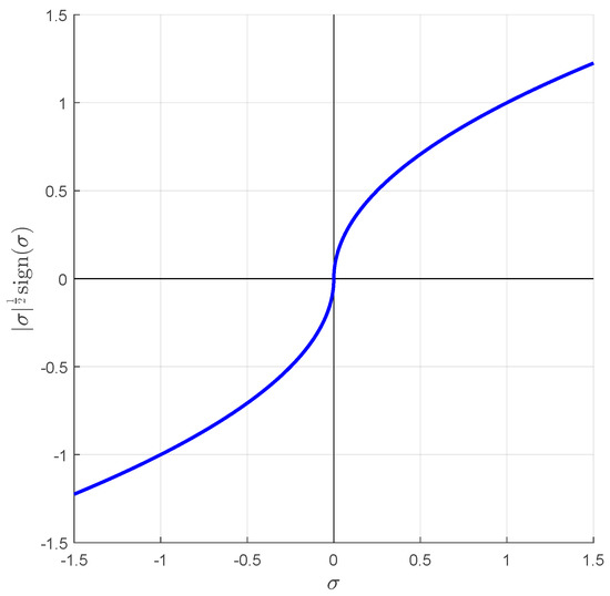
Figure 9.
Switching member of the super twisting sliding mode solution.
Using the small angles approximation to linearize the system in the diving plane, one can derive the sliding condition given by (56) into the following control law:
In this case, a constant depth , is tracked. The coefficients are model parameters and the control input u is analogous to the stern plan defection angle . is a constant sway speed.
The simulation results indeed show dampening of the chattering effect when the STSMC is compared with traditional SMC. However, it should be noted that STSMC displays slightly slower convergence than SMC.
This section demonstrated the use of different sliding mode controls in the case of fully-actuated marine vehicles. As seen in this section, sliding mode control comes in different shapes. However, the two main levers for tweaking the controllers are the definition of the sliding surface itself and the choice of the solution of the sliding condition. Many more examples would be worth adding to this section like the work in [80] where SMC is associated with LOS guidance and Fuzzy Logic in the diving control of an autonomous bio-mimetic dolphin robot as well as [81], which introduces four decoupled SM controllers of different orders in a vehicle with actuated surge, heave, pitch and yaw.
6.2. Sliding Mode Control for Underactuated Vehicles
This section studies the use of SMC in the case of underactuated marine craft. It is notably interested in how the SMC method can be used as a guidance principle and allow compensation of underactuation in the same way LOS does and how SMC can be coupled with external guidance laws.
As a first example, in [82], the model of a -ship tracking horizontal straight lines is studied. Two decoupled controllers are designed one for the surge motion and the other for the yaw motion. Two sliding surfaces are given:
There are multiple points of interest in (58). First, both sliding surfaces are completely defined in the mobile frame. However, because positions in the mobile frame can not be measured, the surfaces are defined in terms of the integral of the velocity on the two axes of the moving frame. This solution is analogous to defining the surfaces in terms of positions but, as shown later, the definition of the surge and sway references matters when it come to tracking trajectories originally defined in the inertial frame. Then, while is of the first order relatively to the integral of u, the second sliding surface is of the second order and defined relatively to the sway speed error instead of the heading angle or the yaw velocity. Therefore, the yaw controller derived from will be based on the sway speed error . Doing so allows the authors to compensate the lack of sway actuation with yaw. This method is very close to the other guidance methods exposed earlier in this review, and it is somewhat equivalent to generating yaw controls based on the lateral error measured on the axis of the moving frame.
The surge and yaw controllers are derived from the respective sliding surfaces and the dynamic model of the system as:
Note that, in the original article, estimated values of the model parameters are used in the control calculations, and the authors left the possibility to consider nonlinear damping. Equation (59) has been simplified for clarity. Equation (59b) is of a different structure than the other control equations seen in this section because it is based on the first time derivation of the sway equation of the dynamic model instead of the first order derivative of the chosen sliding condition solution (58b). Hence, the new speed terms and contain the terms created by this manipulation. Exact definitions of , as well as the gains and can be found in [82]. The dynamic sway equation derivative is used instead of the sliding condition derivative because the latter would require information upon the second order derivative of both the actual and desired sway speeds. Such information is not available in this work.
However, as claimed in [83,84], the solution proposed in [82] does not solve all the tracking problems. In fact, defining the sliding surfaces in terms of the integrals of the speed errors in the moving frame leads to neglecting constant offsets of the desired position signals. To counteract this problem [83,84], redefine the surge and sway velocity references.
First [83], give a similar approach for trajectory tracking of a -ship in the horizontal plane but with modified speed references. To take a possible position offset into account, the desired reference surge and sway speeds are calculated as:
with k a positive constant control parameter. Note that, in the original work [83], two different control parameters and , are mentioned but do not appear in the equations. This work shows that convergence of the surge and sway errors and leads to convergence of the position errors in the inertial frame and . The first order derivative of the second order yaw sliding surface expressed in terms of the integral of the sway error is used for the calculation of the yaw control. Therefore, knowledge about the second order derivative of the desired sway motion is necessary as well as the third order derivative of both desired position signals.
In the same way, Ref. [84] proposes a more global solution than in [82], solving the case of offset trajectories. To do so, new surge and sway speed references are defined as:
where and are controller gains, and and are saturation coefficients chosen relatively to the system’s physics. The definition of the speed references and given by Equation (61) leads to the error equation:
Equation (62) shows that convergence of the speed errors and to zero leads to asymptotic convergence of the position errors and . In fact, the speed errors in Equation (62) behave nearly like sliding surfaces for the positions. The rotation matrix being non-singular, when the speed errors converge to , one obtains:
Equation (63) can be seen as the sliding conditions of the inner loop of the system assuring asymptotic convergence of the position errors the hyperbolic tangent function being used instead of a sign function.
The sliding surfaces used for the dynamic controllers are then given. The sliding surfaces used in [84] are very similar to (58) but with two different control parameters in the yaw surface:
Here, too, the sliding surface used for yaw control is built upon the sway error . Slightly different dynamics than the usual sliding condition (42) are imposed on and :
where are all strictly positive control parameters. This time, the surge and yaw controllers are both calculated with the first order derivations of the sliding surfaces giving:
The newly introduced mass coefficients , , and as well as control parameters and b are given in detail in [84]. The damping surge and yaw coefficients and , respectively, are issued from the damping matrix of the dynamic model. The simulation results show good performance in tracking linear trajectories with or without an offset and circular trajectories.
A more recent example of SMC applied to underactuated vehicles can be found in [10]. In this work, the authors propose a Super Twisting SMC based solution for the problem of leader–follower tracking. The followers are -vehicles following the trajectory set by the mother ship. Three dimensions LOS guidance is used to calculate the approach angle references in pitch and yaw. Then, three decoupled Super Twisting sliding mode controllers are designed for surge, pitch and yaw as well as a fourth one looping back on the forward speed of the mother ship.
For surge control of the follower submarines, a zero-order sliding surface is built upon the surge error with a constant reference . The surface is therefore given as and the Super Twisting formulation of the sliding condition is used as in [78]
with two strictly positive gain parameters and . The definition of the kinematic Super Twisting sliding-mode controller calculating the surge speed consign of the mother ship is similar to this one. The mother ship speed is calculated with the position error kinematic model. More details about mother ship control can be found in the reference [10].
On the other hand, the pitch and yaw controllers are Super Twisting sliding mode controllers using first order terminal sliding surfaces as in [77]. The pitch and yaw sliding surfaces and associated sliding conditions are given by
where all the control parameters are constant and strictly positive.
As seen in the previous examples, the actual control signals , and are derived from the first order derivative of the associated sliding surface and calculated with the corresponding dynamic model equations. For increased robustness to external disturbances, adaptive disturbance terms can be added to the controller equations as shown in [10]. Finally, the four sliding mode controllers are shown to stabilize the tracking errors of the following submarines.
These few examples show that SMC can be used in the underactuated case and displays good performances. In these examples, one can find the idea of using a rotational degree of freedom to compensate the lack of one or two non actuated translations. Sliding mode itself can be used as guidance principle like in [82,83,84] where yaw controls are given as functions of the lateral motion errors using the same idea as in the LOS examples given earlier [30] directly in the sliding surface calculations.
7. Differential Flatness
This section introduces examples of control laws based on differential flatness and applied to both fully-actuated and underactuated marine craft.
The “differential flatness” or, simply, “flatness” is an approach of control-command born in 1991, as a consequence of the work of four French researchers—M. Fliess, J. Lévine, Ph. Martin & P. Rouchon—on the control of an overhead crane [85]. This invention, created from an application, gave rise to a new theory of nonlinear control. It was first formulated in the language of differential algebra [86,87]3. The definition of this property has been reformulated some years later in the formalism of the differential geometry of prolongations and infinite jets [88]. Flatness is a structural property of a to-be-controlled system, which naturally leads to trajectory tracking control. In the linear framework, a flat system is exactly a controllable one, so flatness is a good candidate to be a definition of controllability of nonlinear systems. Flatness is presented in detail in several books [11,89,90,91,92]. The control methodology derived from flatness proceeds in two steps: Firstly, generation of a nominal command from the to-be-followed trajectory by the system, secondly, closing the loop to have robustness properties. The closed loop can be realized in several ways: it can be classical PID, state feedback, LQG/LQR, sliding modes, model-free control… Flatness is sometimes been confused with feedback linearization, partly because, besides its definition, the notion of endogenous feedback and a related notion of linearization were introduced. Remember that flatness corresponds to the notion of state feedback linearization in the case of single-input systems. See [93] for more details on the links between flatness and feedback linearization. About ten years after the appearance of flatness, it has been demonstrated that, during operation, the trajectories of the flat output correspond to that of a linear system in Brunovský form. This property is called “exact feedforward linearization” (thus cannot be confused with feedback linearization). Through this new approach of flatness, it was possible to establish the properties, already observed in practice on applications, of robustness towards parameter errors and perturbations. We can quote [94,95,96] for the theoretical aspects and [97] for the practical aspects of exact feedforward linearization based on differential flatness. The flatness has spread in many domains of control; we can quote here some of them: control of mechanical systems [98], mobile robotics [99], control of electric motors [100], control of chemical reactors [101,102,103] (see references in [11,89,90,92] for more more applications). Besides the academic aspects, the flatness is present in many industrial realizations, too numerous to be all quoted here.
7.1. Differential Flatness Applied in the Fully Actuated Case
One of the few applications of differential flatness theory in the context of marine vehicles can be found in [12]. In this example, a fully-actuated AUV is evaluated on a 6-DOF task. For fully-actuated system, choosing the flat output is pretty straightforward. Nonetheless, this work shows that the model of the fully-actuated AUV is flat for a flat output chosen as the position and orientation vector in the inertial frame. Then, using flatness equations, the inputs of the system are written as functions of the flat output. These expressions are then used to derive a flatness-based linearizing control law using exact feedforward linearization and PD controllers. This work also introduces an additional Kalman disturbances compensation method. The good performances of the method on a 6-DOF task are displayed at the end of this work.
The proof of flatness of the completely actuated AUV given in [12] is a little bit tricky and gives many details that are out the scope of the present work. Let us give a direct proof: the position and orientation vector is the most obvious and natural choice as the flat output. Choosing notably allows for defining the task in terms of desired position, orientation and velocities in the inertial frame, which is both logical and practical in most applications. As in many cases, the flat output found here has a strong signification w.r.t. the control problem as ones want to control . Then, showing the differential flatness of the system is pretty straightforward. In fact, the only variables to express as functions of the flat output are the velocity vector in the body-fixed frame and the propulsion vector . The inverse kinematic model and the dynamic model expressed in the inertial frame constitute self-explanatory demonstrations of the flatness of the system:
Looking at Equation (69), it appears clearly that both the velocity vector and the effort vector can be expressed as functions of the flat output and its derivatives and . The model used to represent fully-actuated marine craft is therefore flat with flat output .
As a consequence of flatness, the nominal open-loop control that achieves trajectory tracking of the reference trajectory of the flat output is expressed by:
Following the reasoning introduced among other in [94] and using the flatness Equation (69), a flatness-based closed-loop controller can be easily defined as:
where is a control function like a PID controller based on the state error and constitutes the exact feedforward linearizing term. Of course, in the fully actuated case, the formulation of the control law built with differential flatness is very close to some of the feedforward linearizing controllers introduced in Section 5.
7.2. Differential Flatness Applied to Underactuated Vehicles
For underactuated vehicles, showing differential flatness is significantly harder. In the marine context, two very promising examples can be found in [11]. Note that, for underactuated systems, the flat output must be of the same dimension as the input which implies that natural relations must exist between the flat output and the rest of the state of the system for it to be flat. In fact, the very last example of chapter 12 in [11] states that the model of an underactuated surface ship is not differentially flat. It is impossible in this example to express all the problem variables as functions of the flat output chosen as the positions in the horizontal plane without the need for integrating a differential equation. Instead, the underactuated surface ship is said to be Liouvillian. Actually, in order to express the heading angle of the vehicle as a function of the flat output, the heading rate must be integrated, therefore introducing integral terms of the flat output and making the system non-flat. More details about the control of Liouvillian systems can be found in [87,104].
However, another very interesting system can be found in [11] as well as in [105]: the Hovercraft system. Arguably, the model used to represent the hovercraft system is very close to the model of an underactuated surface vessel and could even be considered as a special case of the more generic model of the surface ship with selected numerical values of the parameters. The main differences to find between these two models are in the mass distribution and damping approximations. However, the model of the hovercraft is shown to be flat for the flat output in [11,105]. In both examples, equations of flatness allow for calculating surge and yaw controls as function of the desired state, its derivatives up to the fourth order, and PD controllers on the flat output.
8. Conclusions
This work introduces some of the most popular model-based control methods and guidance principles for autonomous marine vehicles, notably feedback and feedforward linearization associated with PID-based control, Line of Sight Guidance, Sliding Mode Control and several other methods. It also tries to give a definition of underactuation of a vehicle relative to the task it is sent on and shows that, even with the right number of actuated degrees of freedom, a vehicle can be ill-actuated relatively to the task meaning that it is not able to generate at the same time all the independent efforts necessary to fulfill the task. A generic example is used to what the consequences of such actuation can be and how some actuated degree of freedom can be used to compensate the lack of another one.
Because the kinematic and dynamic models of the vehicle are nonlinear, model-based linearizations are widely used with underwater vehicles. These methods allow for creating linear or semi-linear closed-loop systems that are much easier to control. The examples presented in this work allow for demonstrating the different solutions for model-based linearization. Either it is only with feedback terms or with a combination of feedback and feedforward terms, model-based linearization shows very good tracking results and, when associated with PID-based controllers, is one of the simplest control methods for these types of vehicles.
The first method dedicated to underactuated vehicles introduced in this work is Line Of Sight Guidance. As a traditional inheritance from naval techniques, LOS guidance has been designed for control of underactuated surface vehicles on waypoint reaching tasks. However, several examples show that the same guidance principles can be used both in 2D and in 3D and for path and trajectory tracking as well. Using a non-diagonal compensation mechanism based on the calculation of new pitch and yaw angle references from sway and heave errors, LOS leads the way for many other guidance and control techniques. To this date, LOS guidance is still predominant both in the literature as well as in the industry. However, LOS guidance alone is not suited for applications where constraints on the orientation of the vehicle are part of the task.
Then, examples of Sliding Mode controllers for both fully-actuated and underactuated vehicles have been introduced. Sliding Mode Control comes in many shapes and both the sliding surfaces and the choice of the sliding condition solution can be tuned to suit desired performances. In the underactuated case, examples of Sliding Mode controllers show the same non-diagonal behavior as LOS does. Indeed, in several examples, the sliding surface of one degree of freedom is calculated upon the error signal of another degree of freedom. Mostly, the yaw sliding surface is calculated with sway errors creating this compensation behavior where yaw is used to cope for the lack of sway actuation.
Finally, differential flatness is also briefly discussed as some examples show that it is a very good candidate for fully-actuated marine craft. This works also gives a hint towards the use of differential flatness on underactuated marine craft as it is carried out on a very similar hovercraft system.
Overall, the guidance and control principles presented in this work represent the main advances of the last few years and can be considered the go-to methods for designing an autonomous marine vehicle. All of them show very good performances and can be applied to almost every marine vehicle regardless of the propulsive configuration.
This work paves the way towards very interesting future research. Notably, the question of controllability of the underactuated marine vehicles relative to their task must be addressed. In the same way, some additional work comparing the different control methods on the same vehicle and on the same task would be interesting to level out the capabilities and performances of each methods. In addition, some more control methods could be added to this study like adaptive controllers or machine learning based methods.
Author Contributions
Conceptualization, L.D., E.D. and O.C.; methodology, L.D., E.D. and O.C.; validation, L.D. and E.D.; formal analysis, L.D.; investigation, L.D.; resources, L.D.; writing—original draft preparation, L.D and E.D.; writing—review and editing, L.D., E.D. and O.C.; supervision, E.D. and O.C.; funding acquisition, E.D. and O.C. All authors have read and agreed to the published version of the manuscript.
Funding
The work of L.D. is funded by research grants from “Région Bretagne” and “Brest métropole”.
Institutional Review Board Statement
Not applicable.
Informed Consent Statement
Not applicable.
Data Availability Statement
The data of this work are only the references cited in the article.
Acknowledgments
The authors thank “Région Bretagne” and “Brest métropôle” for their supports.
Conflicts of Interest
The authors declare no conflict of interest.
Notes
| 1 | For more details about LQR control in this context, see [51]. |
| 2 | Recall that a space of dimension N, and a hypersurface is a geometric object of dimension . |
| 3 | This article is cited more than 3800 times at the date of writing the present work. |
References
- Fossen, T.I. Marine Control Systems: Guidance, Navigation and Control of Ships, Rigs and Underwater Vehicles, 3rd ed.; Marine Cybernetics: Trondheim, Norway, 2002. [Google Scholar]
- Fossen, T.I.; Breivik, M.; Skjetne, R. Line-of-sight path following of underactuated marine craft. Ifac Proc. Vol. 2003, 36, 211–216. [Google Scholar] [CrossRef]
- Breivik, M.; Fossen, T. Principles of Guidance-Based Path Following in 2D and 3D. In Proceedings of the IEEE Conference on Decision and Control (CDC), Seville, Spain, 15 December 2005; pp. 627–634. [Google Scholar]
- Fjellstad, O.E.; Fossen, T. Position and attitude tracking of AUV’s: A quaternion feedback approach. IEEE J. Ocean. Eng. 1994, 19, 512–518. [Google Scholar] [CrossRef]
- Smallwood, D.; Whitcomb, L. Model-based dynamic positioning of underwater robotic vehicles: Theory and experiment. IEEE J. Ocean. Eng. 2004, 29, 169–186. [Google Scholar] [CrossRef]
- Yoerger, D.; Slotine, J.J.E. Robust trajectory control of underwater vehicles. IEEE J. Ocean. Eng. 1985, 10, 462–470. [Google Scholar] [CrossRef]
- Cristi, R.; Papoulias, F.; Healey, A. Adaptive sliding mode control of autonomous underwater vehicles in the dive plane. IEEE J. Ocean. Eng. 1990, 15, 152–160. [Google Scholar] [CrossRef]
- Healey, A.; Lienard, D. Multivariable sliding mode control for autonomous diving and steering of unmanned underwater vehicles. IEEE J. Ocean. Eng. 1993, 18, 327–339. [Google Scholar] [CrossRef]
- Zhihong, M.; Yu, X.H. Terminal sliding mode control of MIMO linear systems. IEEE Trans. Circuits Syst. I 1997, 44, 1065–1070. [Google Scholar] [CrossRef]
- Xia, G.; Zhang, Y.; Zhang, W.; Zhang, K.; Yang, H. Robust adaptive super-twisting sliding mode formation controller for homing of multi-underactuated AUV recovery system with uncertainties. ISA Trans. 2022, 130, 136–151. [Google Scholar] [CrossRef]
- Sira-Ramírez, H.; Agrawal, S.K. Differentially Flat Systems; Marcel Dekker: New York, NY, USA; Basel, Switzerland, 2004. [Google Scholar]
- Rigatos, G.G.; Raffo, G.V.; Siano, P. AUV Control and Navigation with Differential Flatness Theory and Derivative-Free Nonlinear Kalman Filtering. Intell. Ind. Syst. 2017, 3, 29–41. [Google Scholar] [CrossRef]
- Leonard, N. Control synthesis and adaptation for an underactuated autonomous underwater vehicle. IEEE J. Ocean. Eng. 1995, 20, 211–220. [Google Scholar] [CrossRef]
- Lea, R.K.; Allen, R.; Merry, S.L. A comparative study of control techniques for an underwater flight vehicle. Int. J. Syst. Sci. 1999, 30, 947–964. [Google Scholar] [CrossRef]
- Mitchell, A.; McGookin, E.; Murray-Smith, D. Comparison of Control Methods for Autonomous Underwater Vehicles. IFAC Proc. Vol. 2003, 36, 37–42. [Google Scholar] [CrossRef]
- Antonelli, G. Underwater Robots, 4th ed.; Springer International Publishing: Cham, Switzerland, 2018. [Google Scholar]
- Li, H.; Chen, H.; Gao, N.; Aït-Ahmed, N.; Charpentier, J.F.; Benbouzid, M. Ship Dynamic Positioning Control Based on Active Disturbance Rejection Control. J. Mar. Sci. Eng. 2022, 10, 865. [Google Scholar] [CrossRef]
- Fossen, T.I. Guidance and Control of Ocean Vehicles; Wiley: Chichester, NY, USA, 1994. [Google Scholar]
- Lamb, H. Hydrodynamics, 6th ed.; (Unabridged and unaltered republication of the 1932 ed., Cambridge); Dover: New York, NY, USA, 2005. [Google Scholar]
- Imlay, F.H. The Complete Expressions for “Added Mass” of a Rigid Body Moving in an Ideal Fluid; Technical Report 1528; Departement of the Navy, Hydromechanics Laboratory: Arlington, VA, USA, 1961. [Google Scholar]
- Gartner, N.; Richier, M.; Dune, C.; Hugel, V. Hydrodynamic Parameters Estimation Using Varying Forces and Numerical Integration Fitting Method. IEEE Robot. Autom. Lett. 2022, 7, 11713–11719. [Google Scholar] [CrossRef]
- Fossen, T.I.; Johansen, T.A. A Survey of Control Allocation Methods for Ships and Underwater Vehicles. In Proceedings of the 14th Mediterranean Conference on Control and Automation, Ancona, Italy, 28–30 June 2006; pp. 1–6. [Google Scholar]
- Chocron, O.; Vega, E.P.; Benbouzid, M. Dynamic reconfiguration of autonomous underwater vehicles propulsion system using genetic optimization. Ocean. Eng. 2018, 156, 564–579. [Google Scholar] [CrossRef]
- Fossen, T.I.; Pettersen, K.Y. On uniform semiglobal exponential stability (USGES) of proportional line-of-sight guidance laws. Automatica 2014, 50, 2912–2917. [Google Scholar] [CrossRef]
- Breivik, M.; Fossen, T. A unified control concept for autonomous underwater vehicles. In Proceedings of the IEEE American Control Conference (ACC), Minneapolis, MN, USA, 14–16 June 2006. [Google Scholar]
- Calvo, O.; Rozenfeld, A.; Souza, A.; Valenciaga, F.; Puleston, P.; Acosta, G. Experimental results on smooth path tracking with application to pipe surveying on inexpensive AUV. In Proceedings of the IEEE/RSJ International Conference on Intelligent Robots and Systems (IROS’08), Nice, France, 22–26 September 2008; pp. 3647–3653. [Google Scholar]
- Borhaug, E.; Pavlov, A.; Pettersen, K.Y. Integral LOS control for path following of underactuated marine surface vessels in the presence of constant ocean currents. In Proceedings of the 47th IEEE Conference on Decision and Control (CDC), Cancún, Mexico, 9–11 December 2008; pp. 4984–4991. [Google Scholar]
- Caharija, W.; Pettersen, K.Y.; Gravdahl, J.T.; Borhaug, E. Integral LOS guidance for horizontal path following of underactuated autonomous underwater vehicles in the presence of vertical ocean currents. In Proceedings of the IEEE American Control Conference (ACC), Montreal, QC, Canada, 27–29 June 2012; pp. 5427–5434. [Google Scholar]
- Caharija, W.; Pettersen, K.Y.; Gravdahl, J.T.; Borhaug, E. Path following of underactuated autonomous underwater vehicles in the presence of ocean currents. In Proceedings of the 51st IEEE Conference on Decision and Control (CDC), Maui, HI, USA, 10–13 December 2012; pp. 528–535. [Google Scholar]
- Lekkas, A.M.; Fossen, T.I. Minimization of cross-track and along-track errors for path tracking of marine underactuated vehicles. In Proceedings of the 2014 European Control Conference (ECC), Strasbourg, France, 24–27 June 2014; pp. 3004–3010. [Google Scholar]
- Pettersen, K.; Lefeber, E. Way-point tracking control of ships. In Proceedings of the 40th IEEE Conference on Decision and Control (CDC), Orlando, FL, USA, 4–7 December 2001; Voume 1, pp. 940–945. [Google Scholar]
- Xiang, X.; Lapierre, L.; Jouvencel, B. Smooth transition of AUV motion control: From fully-actuated to under-actuated configuration. Robot. Auton. Syst. 2015, 67, 14–22. [Google Scholar] [CrossRef]
- Fossen, T.I.; Lekkas, A.M. Direct and indirect adaptive integral line-of-sight path-following controllers for marine craft exposed to ocean currents. Int. J. Adapt. Control. Signal Process. 2017, 31, 445–463. [Google Scholar] [CrossRef]
- Li, W.; Zhou, Z.; Lou, J.; Zhang, X. A 3D trajectory tracking algorithm for AUV. J. Phys. Conf. Ser. 2021, 1873, 012055. [Google Scholar] [CrossRef]
- Korobov, W. Controllability, stability of some nonlinear systems. Differ. Uravnienje 1973, 9, 466–469. [Google Scholar]
- Brockett, R.W. Feedback invariants for nonlinear systems. In Proceedings of the 7th IFAC World Congress, Helsinki, Finland, 12–16 June 1978; pp. 1115–1120. [Google Scholar]
- Jakubczyk, B.; Respondek, W. On linearization of Control Systems. Bull. L’Acad. Pol. Sci. 1980, 28, 517–522. [Google Scholar]
- Su, R. On the linear equivalents of nonlinear systems. Syst. Control Lett. 1982, 2, 48–52. [Google Scholar] [CrossRef]
- van der Schaft, A.J. Linearization and input-ouput decoupling for general nonlinear systems. Syst. Control Lett. 1984, 5, 27–33. [Google Scholar] [CrossRef]
- Claude, D. Everything you always wanted to know about linearization (but you were afraid to ask). In Algebraic and Geometric Methods in Nonlinear Control Theory; Fliess, M., Hazewinkel, M., Eds.; Reidel: Dordrecht, The Netherlands, 1986. [Google Scholar]
- Charlet, R.; Lévine, J.; Marino, R. On dynamic feedback linearization. Syst. Control Lett. 1989, 13, 143–151. [Google Scholar] [CrossRef]
- Isidori, A. Nonlinear Control Systems: An Introduction, 2nd ed.; Springer: Berlin/Heidelberg, Germany, 1989. [Google Scholar]
- Nijmeijer, H.; van der Schaft, A.J. Nonlinear Dynamical Control Systems; Springer: New York, NY, USA, 1990. [Google Scholar]
- Slotine, J.J.E.; Li, W. Applied Nonlinear Control; Prentice Hall: Upper Saddle River, NJ, USA, 1991. [Google Scholar]
- Isidori, A.; Ruberti, A. On the synthesis of linear input–output responses for nonlinear systems. Syst. Control Lett. 1984, 4, 17–22. [Google Scholar] [CrossRef]
- Pereira da Silva, P.S.; Delaleau, E. Algebraic necessary and sufficient conditions of input–output linearization. Forum Math. 2001, 13, 335–357. [Google Scholar]
- Martin, S.C.; Whitcomb, L.L. Nonlinear Model-Based Tracking Control of Underwater Vehicles With Three Degree-of-Freedom Fully Coupled Dynamical Plant Models: Theory and Experimental Evaluation. IEEE Trans. Control Syst. Technol. 2018, 26, 404–414. [Google Scholar] [CrossRef]
- Hagenmeyer, V.; Delaleau, E. Exact feedforward linearization based on differential flatness. Int. J. Control 2003, 76, 537–556. [Google Scholar] [CrossRef]
- Ortega, R.; Spong, M.W. Adaptive motion control of rigid robots: A tutorial. Automatica 1989, 25, 877–888. [Google Scholar] [CrossRef]
- Nguyen-Tuong, D.; Seeger, M.; Peters, J. Computed torque control with nonparametric regression models. In Proceedings of the IEEE American Control Conference (ACC), Seattle, WA, USA, 11–13 June 2008; pp. 212–217. [Google Scholar]
- Wahl, A.; Gilles, E.D. Model predictive versus linear quadratic control for the tracking problem of automatic river navigation. In Proceedings of the 5th European Control Conference (ECC), Karlsruhe, Germany, 31 August–3 September 1999; pp. 1137–1142. [Google Scholar]
- Fossen, T.; Sagatun, S. Adaptive control of nonlinear underwater robotic systems. In Proceedings of the IEEE International Conference on Robotics and Automation (ICRA), Sacramento, CA, USA, 9–11 April 1991; Volume 2, pp. 1687–1694. [Google Scholar]
- Yuh, J.; Nie, J.; Lee, C.S.G. Experimental study on adaptive control of underwater robots. In Proceedings of the IEEE International Conference on Robotics and Automation (ICRA), Detroit, MI, USA, 10–15 May 1999; pp. 393–398. [Google Scholar]
- Antonelli, G.; Caccavale, F.; Chiaverini, S.; Fusco, G. On the use of integral control actions for autonomous underwater vehicles. In Proceedings of the European Control Conference (ECC), Porto, Portugal, 4–7 September 2001; pp. 1186–1191. [Google Scholar]
- Antonelli, G.; Caccavale, F.; Chiaverini, S.; Fusco, G. A novel adaptive control law for underwater vehicles. IEEE Trans. Control Syst. Technol. 2003, 11, 221–232. [Google Scholar] [CrossRef]
- Alonge, F.; D’Ippolito, F.; Raimondi, F. Trajectory Tracking of Underactuated Underwater Vehicles. In Proceedings of the 40th IEEE Conference on Decision and Control (CDC), Orlando, FL, USA, 4–7 December 2001. [Google Scholar]
- Vega, E.P.; Chocron, O.; Ferreira, J.V.; Benbouzid, M.; Meirelles, P.S. Evaluation of AUV Fixed and Vectorial Propulsion Systems with Dynamic Simulation and Non-linear Control. In Proceedings of the 41st Annual Conference of the IEEE Industrial Electronics Society (IECON2015), Yokohama, Japan, 9–12 November 2015. [Google Scholar]
- Degorre, L.; Chocron, O.; Delaleau, E. Une approche générique de la commande basée modèle des AUV sous-actionnés. In Proceedings of the 25e Congrès Français de Mécanique, Nantes, France, 29 August–2 September 2022. [Google Scholar]
- Flügge-Lotz, I. Discontinuous Automatic Control; Princeton University Press: Princeton, NJ, USA, 1953. [Google Scholar]
- Emelyanov, S.V. A technique to develop complex control by using only the error signal of control variable and its first derivatives. Autom. Telemekhanika 1957, 18, 873–885. [Google Scholar]
- Aizerman, M.A.; Gantmacher, F.R. On some features of switchings in nonlinear control with a piecewise smooth response of the nonlinear element. Autom. Telemekhanika 1957, 18. [Google Scholar]
- Flügge-Lotz, I.; Taylor, C.; Lindberg, H. Investigations on Nonlinear Control; NACA: Boston, MA, USA, 1958; p. 1391. [Google Scholar]
- Grishchenko, M.; Ivanov, V.; Mavritayn, V.F. Multivariable Variable Structure Control Systems. In Proceedings of the 3rd All-Union Conference Automatic Control, Geneva, Switzerland, 1–13 September 1958. [Google Scholar]
- Shigin Ye, K. On improvement of Transient Processes in Variable Parameter Correcting Elements. Avtom. Telemekhanika 1958, 19, 306–312. [Google Scholar]
- Cypkin, J.Z. Théorie des Asservissements par Plus-ou-Moins; Dunod: Paris, France, 1962; (Translated from Russian). [Google Scholar]
- Emelyanov, S.V. Variable Structure Control Systems; Nauka: Moscow, Russia, 1967. (In Russian) [Google Scholar]
- Itkis, U. Control Systems of Variable Structures; Wiley: New York, NY, USA, 1976. [Google Scholar]
- Utkin, V.I. Sliding Modes and their Applications in Variable Structure System; Ed. MIR: Moscow, Russia, 1978. [Google Scholar]
- Utkin, V.I. Discontinuous Control Systems: State of Art in Theory and Application. IFAC Proc. Vol. 1987, 20, 25–44. [Google Scholar] [CrossRef]
- Filippov, A.F. Differential Equations with Discontinuous Righthand Sides, First version published as “Differential equations with discontinuous right par”. Mathematical Proceedings I, 1961; Springer: Dordrecht, The Netherlands, 1988. (In Russian) [Google Scholar]
- Sira-Ramírez, H. Sliding Mode Control: The Delta-Sigma Modulation Approach; Birkhäuser: Cham, Switzerland, 2015. [Google Scholar]
- Slotine, J.J.E. Tracking Control of Nonlinear Systems Using Sliding Surfaces. Ph.D. Thesis, Massachusetts Institute of Technology, Cambridge, MA, USA, 1983. [Google Scholar]
- Slotine, J.J.E.; Sastry, S.S. Tracking control of nonlinear systems using sliding surfaces, with application to robot manipulators. Int. J. Control 1983, 38, 465–492. [Google Scholar] [CrossRef]
- Yoerger, D.; Slotine, J.J.E. Nonlinear Trajectory Control of Autonomous Underwater Vehicule Using the Sliding Methodology. In Proceedings of the IEEE Conference OCEANS, Washington, DC, USA, 10–12 September 1984. [Google Scholar]
- Levant, A. Sliding order and sliding accuracy in sliding mode control. Int. J. Control 1993, 58, 1247–1263. [Google Scholar] [CrossRef]
- Young, K.; Utkin, V.; Ozguner, U. A control engineer’s guide to sliding mode control. IEEE Trans. Control Syst. Technol. 1999, 7, 328–342. [Google Scholar] [CrossRef]
- Londhe, P.S.; Dhadekar, D.D.; Patre, B.M.; Waghmare, L.M. Non-singular terminal sliding mode control for robust trajectory tracking control of an autonomous underwater vehicle. In Proceedings of the Indian Control Conference (ICC), Guwahati, India, 4–6 January 2017; pp. 443–449. [Google Scholar]
- Anandan, M.S.; Lal Priya, P.S. Super Twisting Sliding Mode Controller for a Diving Autopilot. In Proceedings of the 2nd International Conference on Power, Control and Computing Technologies (ICPC2T), Raipur, India, 1–3 March 2022; pp. 1–6. [Google Scholar]
- Jayakrishnan, H. Position and Attitude control of a Quadrotor UAV using Super Twisting Sliding Mode. IFAC-PapersOnLine 2016, 49, 284–289. [Google Scholar] [CrossRef]
- Yu, J.; Liu, J.; Wu, Z.; Fang, H. Depth Control of a Bioinspired Robotic Dolphin Based on Sliding-Mode Fuzzy Control Method. IEEE Trans. Ind. Electron. 2018, 65, 2429–2438. [Google Scholar] [CrossRef]
- Shrivastava, A.; Karthikeyan, M.; Rajagopal, P. Modelling and Motion Control of an Underactuated Autonomous Underwater Vehicle. In Proceedings of the 6th Asia-Pacific Conference on Intelligent Robot Systems (ACIRS), Tokyo, Japan, 16–18 July 2021; pp. 62–68. [Google Scholar]
- Ashrafiuon, H.; Muske, K.R. Sliding mode tracking control of surface vessels. In Proceedings of the IEEE American Control Conference (ACC), Seattle, WA, USA, 11–13 June 2008; pp. 556–561. [Google Scholar]
- Yu, R.; Zhu, Q.; Xia, G.; Liu, Z. Sliding mode tracking control of an underactuated surface vessel. IET Control Theory Appl. 2012, 6, 461. [Google Scholar] [CrossRef]
- Elmokadem, T.; Zribi, M.; Youcef-Toumi, K. Trajectory tracking sliding mode control of underactuated AUVs. Nonlinear Dyn. 2016, 84, 1079–1091. [Google Scholar] [CrossRef]
- Fliess, M.; Lévine, J.; Rouchon, P. Asimplified approach of crane control via generalized state-space model. In Proceedings of the 30th IEEE Conference on Decision and Control (CDC), Brighton, UK, 11–13 December 1991; pp. 736–741. [Google Scholar]
- Fliess, M.; Lévine, J.; Martin, P.; Rouchon, P. Sur les systèmes non linéaires différentiellement plats. Comptes Rendus L’Acad. Sci. Paris 1992, 315, 619–624. [Google Scholar]
- Fliess, M.; Lévine, J.; Martin, P.; Rouchon, P. Flatness and defect of nonlinear systems: Introductory theory and examples. Int. J. Control 1995, 61, 1327–1361. [Google Scholar] [CrossRef]
- Fliess, M.; Lévine, J.; Martin, P.; Rouchon, P. A Lie-Bäcklund approach to equivalence and flatness of nonlinear systems. IEEE Trans. Autom. Control 1999, 44, 922–937. [Google Scholar] [CrossRef]
- Hagenmeyer, V. Robust Nonlnear Tracking Controlbased on Differential Flatness; Fortschritt-Berichte; VDI Verlag: Düsseldorf, Germany, 2003; Volume 8. [Google Scholar]
- Lévine, J. Analysis and Control of Nonlinear Systems: A Flatness-Based Approach; Springer: Berlin/Heildelberg, Germany, 2009. [Google Scholar]
- Rigatos, G.G. Nonlinear Filtering and Control Using Differential Flatness Approaches: Applications to Electromechanical Systems; Springer International Publishing: Cham, Switzerland, 2015. [Google Scholar]
- Rudolph, J. Flatness-Based Control: An Introduction; Shaker Verlag: Düren, Germany, 2021. [Google Scholar]
- Fliess, M.; Lévine, J.; Martin, P.; Olivier, F.; Rouchon, P. Flatness and dynamic feedback linearizability: Two approaches. In Proceedings of the 3rd European Control Conference (ECC), Roma, Italy, 5–8 September 1995. [Google Scholar]
- Hagenmeyer, V.; Delaleau, E. Robustness Analysis of Exact Feedforward Linearization based on differential flatness. Automatica 2003, 39, 1941–1946. [Google Scholar] [CrossRef]
- Hagenmeyer, V.; Delaleau, E. Continuous-time nonlinear flatness-based predictive control: An exact feedforward linearisation setting with an induction drive example. Int. J. Control 2008, 81, 1645–1663. [Google Scholar] [CrossRef]
- Hagenmeyer, V.; Delaleau, E. Robustness Analysis with Respect to Exogenous Perturbations for Flatness-Based Exact Feedforward Linearization. IEEE Trans. Autom. Control 2010, 55, 727–731. [Google Scholar] [CrossRef]
- Delaleau, E.; Hagenmeyer, V. Commande prédictive non linéaire fondée sur la platitude du moteur à induction: Application au positionnement de précision. J. Eur. Syst. Autom. 2002, 36, 737–748. [Google Scholar]
- Bennani, M.K.; Rouchon, P. Robust stabilization of flat and chained systems. In Proceedings of the 3rd European Control Conference (ECC), Roma, Italy, 5–8 September 1995; pp. 1781–1786. [Google Scholar]
- Fliess, M.; Lévine, J.; Martin, P.; Rouchon, P. Flatness and motion planning: The car with n trailers. In Proceedings of the 2nd European Control Conference (ECC), Groningen, The Netherlands, 28 June–1 July 1993; pp. 1518–1522. [Google Scholar]
- Chelouah, A.; Delaleau, E.; Martin, P.; Rouchon, P. Differential flatness and control of induction motors. In Proceedings of the Symposium on Control, Optimization and Supervision, Lille, France, 9–12 July 1996; Computational Engineering in Systems Applications IMACS Multiconference. Borne, P., Staroswiecki, M., Cassar, J.P., El Khattabi, S., Eds.; Gerf EC Lille, Villeneuve d’Ascq: Villeneuve-d’Ascq, France, 1996; pp. 80–85, (Invited Paper). [Google Scholar]
- Rouchon, P. Vibrational control and flatness of chemical reactors. In Proceedings of the Symposium on Control, Optimization and Supervision, Lille, France, 9–12 July 1996; Computational Engineering in Systems Applications IMACS Multiconference. Borne, P., Staroswiecki, M., Cassar, J.P., El Khattabi, S., Eds.; Ecole Centrale de Lille: Villeneuve-d’Ascq, France, 1996; pp. 211–212. [Google Scholar]
- Rothfuss, R.; Rudolph, J.; Zeitz, M. Flatness based control of a nonlinear chemical reactor model. Automatica 1996, 32, 1433–1439. [Google Scholar] [CrossRef]
- Hagenmeyer, V.; Nohr, M. Flatness-based two-degree-of-freedom control of industrial semi-batch reactors. In Control and Observer Design for Nonlinear Finite and Infinite Dimensional Systems; Springer: Berlin/Heildelberg, Germany, 2005. [Google Scholar]
- Chelouah, A.; Petitot, M. Finitely discretizable nonlinear systems: Concepts and definitions. In Proceedings of the 34th IEEE Conference on Decision and Control (CDC), New Orleans, LA, USA, 13–15 December 1995; Volume 1, pp. 19–24. [Google Scholar]
- Rigatos, G.G. Differential Flatness Theory and Flatness-Based Control. In Nonlinear Control and Filtering Using Differential Flatness Approaches: Applications to Electromechanical Systems; Rigatos, G.G., Ed.; Springer International Publishing: Cham, Switzerland, 2015; pp. 47–101. [Google Scholar]


Disclaimer/Publisher’s Note: The statements, opinions and data contained in all publications are solely those of the individual author(s) and contributor(s) and not of MDPI and/or the editor(s). MDPI and/or the editor(s) disclaim responsibility for any injury to people or property resulting from any ideas, methods, instructions or products referred to in the content. |
© 2023 by the authors. Licensee MDPI, Basel, Switzerland. This article is an open access article distributed under the terms and conditions of the Creative Commons Attribution (CC BY) license (https://creativecommons.org/licenses/by/4.0/).