Article

Analysis of Interaction between Interior and Exterior Wall Corrosion Defects

1
School of Chemistry and Chemical Engineering, Yulin University, Yulin 719000, China
2
Shaanxi Key Laboratory of Low Metamorphic Coal Clean Utilization, Yulin 719000, China
3
Key Laboratory of Fluid Transmission Technology of Zhejiang Province, Zhejiang Sci-Tech University, Hangzhou 310018, China
*
Author to whom correspondence should be addressed.
J. Mar. Sci. Eng. 2023, 11(3), 502; https://doi.org/10.3390/jmse11030502
Submission received: 4 February 2023 / Revised: 22 February 2023 / Accepted: 23 February 2023 / Published: 25 February 2023

Abstract

:
With the increase in oil and gas pipe mileage, various corrosion defects inevitably occur, so the mechanisms and the applicability of the interaction corrosion defects are investigated. The ANSYS Workbench software is used to study the three double defect pipe models based on the exterior wall, the interior wall, and the interior and exterior wall. First, the distribution of the stress nephogram is investigated. Second, the failure pressure is obtained through the load step based on the variety of the failure pressure. Finally, the critical distance formula of the different types of double defect pipe models is fitted using MATLAB software, and its applicability and accuracy are verified. The results show that the equivalent stress is divided into two areas; with increasing defect depth and defect length, the critical distance increases and the growth rate increases; by fitting the critical distance formula of the three double defect pipe models, the multiple function formula of defect depth and defect length under different defect location distribution is obtained, with high accuracy. The critical distance ratio is introduced to compare 150 sets of data of the 3 models for conservative calculation; the three models perform well in the critical distance ratio and the double defect pipe model based on the exterior wall is the most conservative.

1. Introduction

As an extremely important strategic resource, natural gas and oil are also the pillar of economic development, so the normal operation of all industries cannot be separated from them; these factors promote the rapid development of the natural gas and oil industries. For all countries, the safe transportation of natural gas and oil through special pipes is an important basis for their utilization and pipes are an important link to realize energy utilization.
Corrosion accounts for about 40% of all safety accidents in natural gas and oil pipes. If some safety accidents such as corrosion perforation and leakage occur in the underground gas and oil transportation pipe, it is necessary to repair, inspect, and evaluate these pipe sections, which will not only lead to the shutdown of enterprises, but also cause incalculable losses to economic development and to a certain extent affect social security and stability. Therefore, all countries attach great importance to the safe transportation of natural gas and oil [1]. To ensure the safe and stable transportation of natural gas and oil resources, most of the natural gas and oil pipes currently in service are buried pipes; although this can save the land area and prevent them from being directly exposed to the sun, it will be affected by soil microorganisms and outer complex environments, resulting in the exterior wall corrosion. At the same time, due to the influence of the interior transportation medium of the pipe, the interior wall corrosion impact is inevitable and various corrosion defects such as rectangular, spherical, ellipsoidal, shuttle, etc. will be formed on the interior and exterior wall of the pipe. Under the dual influence of corrosion defects based on the interior and exterior wall, the corrosion rate of the pipe increases and the service life and failure pressure are greatly reduced, which brings great challenges to the stable transportation of oil and gas resources [2]. Some safety accidents often occur in natural gas and oil pipes; the interior and exterior wall of many underground transportation pipes have different degrees of corrosion defects. Moreover, at the present stage, the pipe detection means are insufficient, the detection costs are expensive, most enterprises do not pay enough attention to the pipe safety detection, and there is no unified maintenance and repair system, which will cause huge economic losses and also hide many safety dangers [3]. To avoid or reduce safety accidents caused by corrosion and ensure the safety of natural gas and oil transport pipes, the world should formulate evaluation standards for the failure pressure of corroded pipes, establish and improve relevant systems and regulations, and require strict compliance.
In view of whether the pipe can meet the conditions for continuous safe and stable operations, by analyzing the degree of corrosion defects on the interior and exterior wall and the failure pressure, one can select and adopt reasonable detection methods to evaluate the safety of the transportation pipe, which is the problem to be solved by studying the failure pressure of the interior and exterior wall corrosion defects and the interaction between them. Due to its advantages of high accuracy, simple operation, and low cost, the FEM method plays an important role in the safety assessment of corroded pipelines [4]. Moustabchir et al. [5,6] studied the stress distribution of semi-elliptical longitudinal defects by combining the strain gauge experimental method and FEM method, and the experimental results were in good agreement with FEM results. Fekete and Varga [7] investigated the impact of the defect corrosion ratio of length to width on their failure behavior by numerical simulation and verified it with experimental data. Duane and Roy [8] considered the influence of defect geometry, proposed a new method for calculating pipeline failure pressure, and verified it using the test method, with high precision. Hosseini et al. [9] conducted experimental research on X52 corrosion defect pipe steel and compared it with the existing API579 evaluation criteria. Based on FEM analysis, Ma et al. [10] established a new failure pressure calculation formula and verified it with blast test data; the results show that the new formula has a high precision and can calculate the failure pressure of high-tensile steel very well. Sun et al. [11] deduced a new calculation formula of failure pressure and the Folias bulging factor by using FEM analysis and, compared with the common failure pressure evaluation criteria and the full blast test results, the results were in good agreement. Yeom et al. [12] used FEM to predict the failure pressure of the X70 pipe, established a new failure pressure calculation formula, and verified it with the full-size blast test data, with high precision. Shuai et al. [13] established a new failure pressure calculation formula using FEM, and, compared to the common failure pressure evaluation model, the model had a small error, high accuracy, and good reliability. Mokhtari and Melchers [14] proposed an improved failure pressure evaluation criterion considering volume loss for the first time in view of the conservative phenomenon of the traditional failure pressure evaluation criterion; the results showed that the criterion is highly accurate and stable. Majid et al. [15] have carried out experiments and hydrodynamic prediction analysis on the corrosion failure process of the X42 pipe steel, which can clearly explain its corrosion mechanism. Caleyo et al. [16] used the probability distribution method to model, evaluated the reliability of the relevant variables, and proposed a reliability evaluation method for the remaining life of the corrosion defect pipe model; the results showed that the precision was higher. Cerit et al. [17,18] investigated the stress distribution of elliptical corrosion defects under torsion by using FEM analysis and established the equation of the stress concentration coefficient; the results showed that the aspect ratio of elliptical defects was the main factor influencing the stress concentration coefficient and the greater the aspect ratio, the greater the maximum stress and the lower the bearing capacity. Xu and Cheng [19] predicted the failure pressure of the corrosion defect pipe models of different steel grades with the help of FEM analysis and compared it with three commonly used failure pressure evaluation criteria; the results showed that the more the defect depth, the lower the steel grade, the lower the residual strength of pipes, and the more dangerous it was. Xu and Cheng [20] studied the corrosion mechanism of pipes through mechanical-electrochemical coupling technology and the error between the simulation results and experimental results is very small; the results show that when elastic deformation occurs in the defect, the coupling effect on corrosion can be ignored; when plastic deformation occurs in the defect, the coupling effect has a greater impact on the corrosion and the corrosion intensifies. Zelmati et al. [21] carried out life prediction for X70 pipe steel with corrosion defects and conducted the correlation study of four failure pressure evaluation criteria by introducing the parameter reliability index. Many researchers have performed a much research on the corrosion process, but mainly on single corrosion defects.
For double defects, Chouchaoui and Pick [22,23] first studied circumferential double defect pipe model and predicted their failure pressure. Benjamin et al. [24,25] elaborated on the interaction phenomenon of multiple corrosion defects pipe models, established a pipeline test database with the help of the full-size blasting test, and compared the database with the common failure pressure evaluation criteria with high accuracy. Chen et al. [26] investigated the failure process of the X80 double defect pipe model, proposed a new failure pressure calculation formula, and compared it with the test results; the results indicated that the formula has a high accuracy. Bedairi et al. [27] used FEM analysis to establish the failure pressure calculation formula of a mixed defect pipeline that cannot be directly solved by the conventional failure pressure specification and verified it with the help of the blast test; the results showed that the method was very applicable. Al-Owaisi et al. [28] studied the interaction mechanism of double defect pipe models with the help of FEM analysis and proposed failure criteria for the interaction corrosion defects; the results showed that the defect location and defect spacing determined the interaction between the defects. Soares et al. [29] adopted FEM to deduce the failure pressure calculation formula of double defect pipe models under the coupling effect of pressure and thermal stress; the results showed that thermal stress has a great influence on failure pressure. Sun and Cheng [30] adopted FEM to deduce the failure pressure of the X46, X60, and X80 with longitudinal and circumferential double defect pipe models; the results showed that the defect interaction is independent of the steel grade, is only related to the defect geometric dimension and defect spacing, and that the defect spacing has a critical value. Sun and Cheng [31] studied the corrosion behavior of the X46 double defect pipe model under mechanical-electrochemical coupling action; the results showed that the stress near the defect was larger, the current density was higher, and the corrosion rate was accelerated. Sun et al. [32] proposed a new failure pressure evaluation formula, despite the fact that the commonly used failure pressure evaluation criteria could not accurately assess the circumferential corrosion defects pipe and verified it with the full-size blasting test; the results showed that the error between the formula calculation results and the blasting test results was very small, with good accuracy and applicability. Al-Owaisi et al. [33] conducted a tested study on the failure process of single and double defect pipe models on the X52 and X60 pipeline, and compared the experimental burst pressure with the common failure pressure evaluation criteria by studying the two factors of defect shape and defect direction; the impact of defect shape on its interaction was examined and the results showed that the impact of defect shape on its interaction was negligible and the defect direction had a significant effect on its interaction. Chen et al. [34] predicted the single and double corrosion defect failure behavior of high-strength X80 pipe steel and compared it with the test results and common failure pressure evaluation criteria, which verified the precision and applicability of the prediction results. Lo et al. [35] took a longitudinally interacting defect pipeline as the research object and used the ANN model to train the data obtained from FEM to obtain the residual strength calculation formula, which was verified by the test data, with high accuracy. Chen et al. [36] predicted the residual strength of axially adjacent submarine double defect pipe model, analyzed the interaction mechanism between the defects, and established a new formula for calculating failure pressure with high precision. Li et al. [37] investigated the failure behavior of double defect and corrosion defect groups’ pipe models, studied their interaction mechanisms, and compared them with common failure pressure evaluation criteria with high precision. There are few studies on the double defect pipe model as most studies are qualitative analyses; only the equivalent stress or failure pressure of the pipes are studied, the applicability is very limited, and the mechanism and applicability of interaction corrosion defects are relatively few. In addition, most researchers are focused on exterior wall corrosion, while research on interior wall corrosion and interior and exterior wall corrosion is relatively less [38].
The ASME B31G evaluation criteria, based on comprehensive disciplines such as elastic-plastic mechanics, establishes the failure pressure prediction equation, which is the most recognized and earliest applied failure pressure evaluation method for corroded pipelines in the world and plays an important role in the safe operation of corroded pipelines. However, the ASME B31G evaluation criterion also has some shortcomings: it is only applicable to single axial corrosion defects, not to multiple corrosion defects, and it is unable to study the interaction mechanism between corrosion defects; the prediction accuracy of failure pressure is relatively high in low steel grade pipes with defects and the accuracy cannot meet the requirements in high steel grade pipes with defects; the forecast results are conservative, which leads to an increase in economic costs. Therefore, in order to solve the above problems, this paper takes X100 high grade steel pipeline as the research object, studies the interaction mechanisms between double rectangular corrosion defects, fits the critical distance formula of the double rectangular corrosion defects pipeline model, and verifies its applicability and accuracy.
Therefore, in this paper, the ANSYS Workbench software is used to study the three double defect pipe models based on the exterior wall, the interior wall, and the interior and exterior wall. First, the distribution of the stress nephogram is investigated. Second, the failure pressure is obtained through the load step based on the variety of the failure pressure, the critical distance of the corrosion defect is obtained through the judgment standard of 5% critical influence, and the impact of defect geometric factors such as depth, length, and spacing on the critical distance is examined. Finally, the critical distance formula of different types of double defect pipe models is fitted using MATLAB software, and their applicability and accuracy are verified. The research has good economic benefits for the safety maintenance and management of natural gas and oil pipes.

2. Establishment of FEM Model

2.1. Establishment and Parameters of the Geometric Model

The selected material for the pipe is the X100 pipe steel and the size of the model is D320 × 20. According to the Saint-Venant principle [38]:
Δ L 2.5 R t = 56.5685   mm
where ΔL is the pipe length affected by the end effect, mm; R is the exterior radius, mm; t is the pipe wall thickness, mm.
Taking the rectangular corrosion defect as the research object, the three double defect pipe models based on the exterior wall, the interior wall, and the interior and exterior wall are analyzed. The length of pipe model is 1200 mm, the diameter is 320 mm, and the thickness is 20 mm. The SolidWorks software is used to cut the defect by rotation to form corrosion pits, the defect exists in the middle of the pipe, and the length of the pipe at both ends is much greater than ΔL, so the end effect is avoided. Since the model is geometrically axisymmetric, so in order to shorten the calculation time, half of the pipe is taken as the research model [7,9]. The geometric parameters of the pipe section model are illustrated in Table 1.

2.2. FEM Model

The precision simulated by the model is related to the number of meshes, but to facilitate operation and maintain calculation accuracy, the model is automatically meshed for the established model and the local meshes are densified for structural discontinuity [14,27]. In order to study the sensitivity of the mesh, 2, 3, 4, and 5 layers of mesh were divided along the direction of the pipe wall thickness, and the effect of the different mesh layers on the maximum equivalent stress was investigated, as shown in Figure 1. It can be seen that when the number of layers was 2, the maximum equivalent stress had an extreme point, which was inconsistent with the change trend of the material stress, and the accuracy was low. When the number of layers was greater than 2, the change trend of the maximum equivalent stress was basically the same, there was no extreme point, and the accuracy had met the requirements. Therefore, the number of mesh layers is 3, the number of nodes is 116,506, and the number of elements is 62,968.

2.2.1. Model Constraints

Due to the geometric symmetry and load symmetry of the model, the displacement constraint on the X-axis direction of both ends of the pipe was 0; we applied a displacement constraint of 0 in the Y-axis direction to the central symmetry plane.

2.2.2. Application of Load

For the application of load, in order to facilitate and simplify the operation and analysis of FEM, and ensure the accuracy of its results, only the impact of the interior pressure load on the pipe needed to be considered and other loads were ignored [10,16,30].

2.2.3. Failure Pressure Solution

Before solving the results, the load step analysis was set for the model. Based on the elastic failure criterion, a value close to yield strength was found in the load step calculation table for analysis and the failure pressure of the double defect pipe model was solved.

2.3. Failure Criterion

The elastic failure criterion took the interior wall yield as the judgment condition for the failure pressure of the container; that is, the elastic failure occurred [6,20]. The maximum stress near the pipe defect reached yield strength, the pipe was considered to have failed. This criterion only considered the elastic stress state, which was conservative. Therefore, when calculating the failure pressure, the failure criteria adopted were all elastic failure criteria.

2.4. Verification of FEM Results

In order to verify the accuracy and applicability of the established FEM model, three groups of blasting test data of X100 pipeline steel pipeline with defects were used [39,40]. The geometric parameters and FEM failure pressure of the pipeline are shown in Table 2. The relative error and pressure ratio of parameters were introduced, in which the relative error = (bursting pressure − FEM failure pressure)/bursting pressure, and the pressure ratio = bursting pressure/FEM failure pressure. It can be seen that the maximum relative error of the FEM method was 8.8%, the minimum relative error was 5.3%, and the average relative error was 6.6%. The FEM failure pressure was very close to the bursting pressure and the pressure ratio basically fluctuated around 1; the results showed that the established FEM model had a high accuracy and could well predict the failure pressure of pipeline with defects.
Where D represents pipe diameter, mm, t represents pipe wall thickness, mm, a represents defect depth, mm, and b represents defect length, mm.

2.5. Critical Distance Calculation Method

The failure pressure Pd of the double defect pipe model was calculated using the above solution method. By comparing it with the failure pressure Ps of the single defect pipe model, the following formula was used to determine whether the interference effect had occurred. When the critical influence factor was less than 5%, it was considered that there was no interference effect between the two defects in this case and that no interference phenomenon occurred, so then both defects can be considered separate defects [38].
ω = Δ P / P d = P d P s / P d × 100 % 5 %
where ω is the critical influence factor; Pd is failure pressure of the double defect pipe model calculated using FEM, MPa; Ps is the failure pressure of the single defect pipe model calculated using FEM, MPa.

2.6. Example of the Critical Distance Calculation

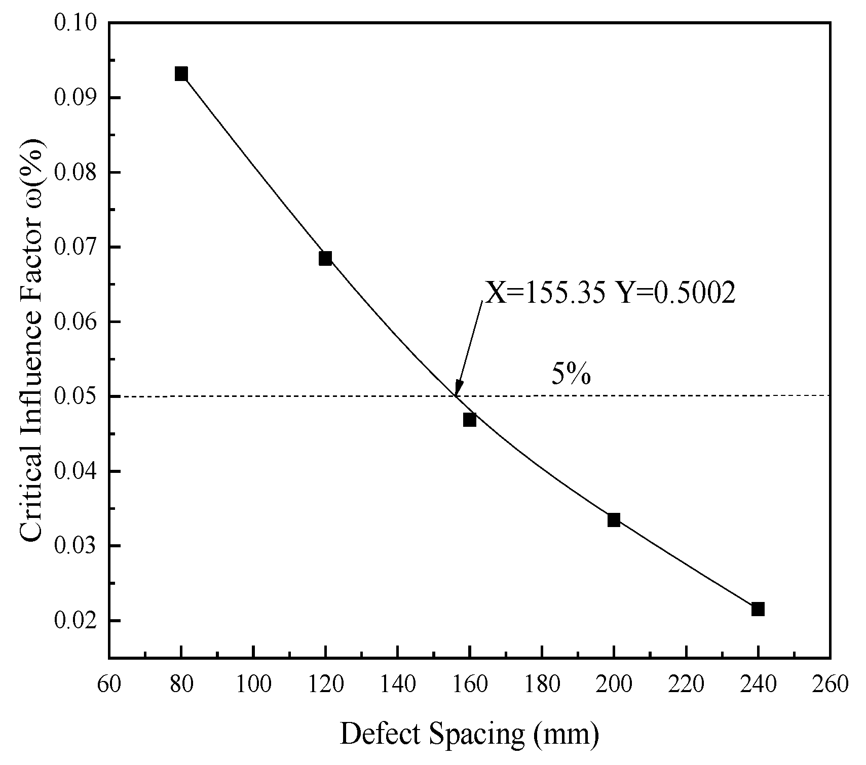
Taking the double defect pipe model based on the exterior wall as an example, the defect depth of the left exterior wall a1/t = 0.6 and the defect depth of the right exterior wall a2/t = 0.5. The defect spacing was 80, 120, 160, 200, and 240 mm. The calculated failure pressure and the critical influence factor are shown in Table 3. The influence of defect spacing on critical influence factor is shown in Figure 2. The specified critical impact factor ω = 5% is the standard and the critical distance is 155.35 mm.

3. Results of the FEM Analysis

The three double defect pipe models is based on the exterior wall, the interior wall, and the interior and exterior wall. First, the distribution of the stress nephogram is investigated. Second, the failure pressure is obtained through the load step based on the variety of the failure pressure, the critical distance of corrosion defect is obtained through the judgment standard of 5% critical influence, and the impact of defect geometric factors such as depth, length, and spacing on the critical distance is examined. Finally, the critical distance formula of different types of double defect pipe model is fitted using MATLAB software, and its applicability and accuracy are verified.

3.1. Geometric Model and Stress Nephogram of Different Double Defect Pipe Models

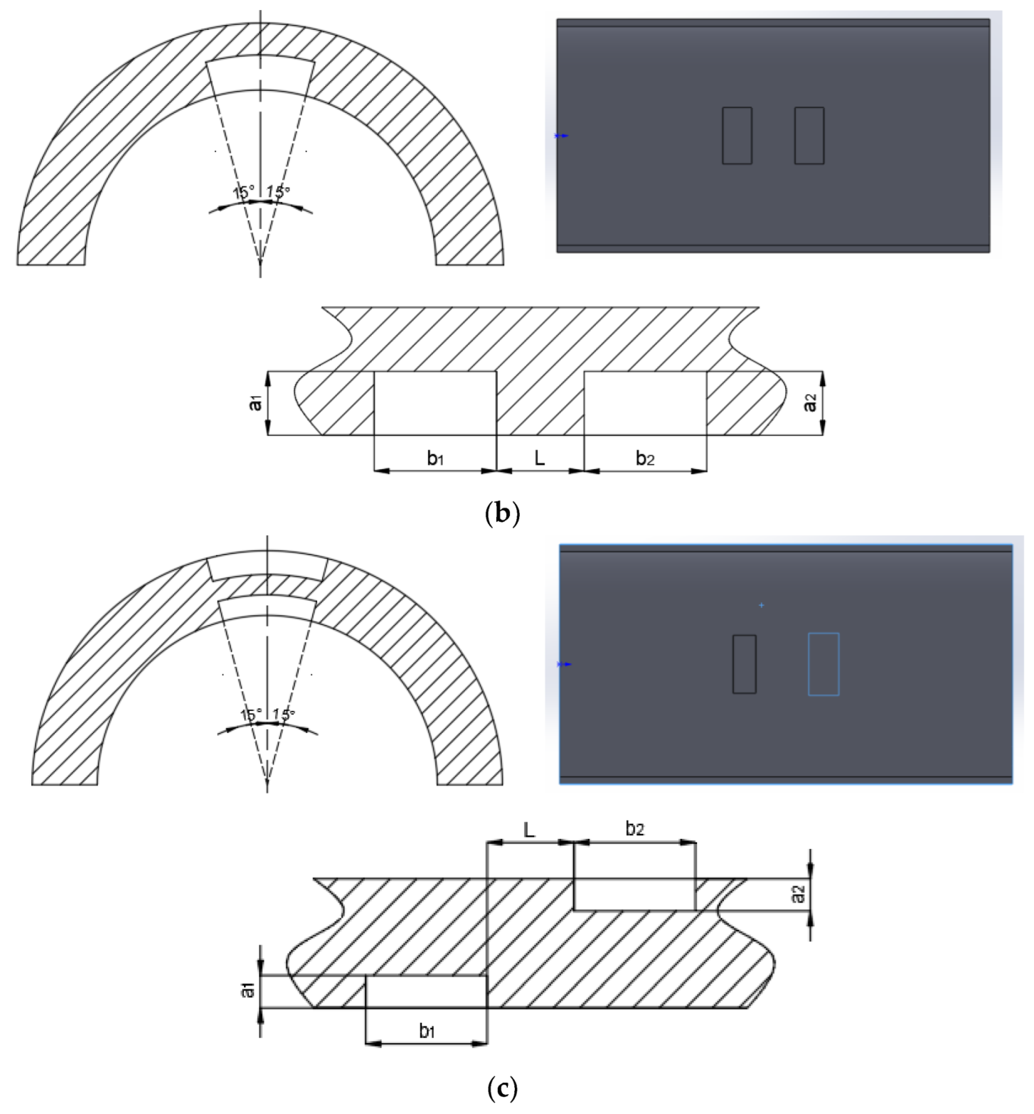
Using the rotary cutting function in SolidWorks software, the double-rectangular corrosion defect pit pipe models of the exterior wall, interior wall, and interior and exterior walls are established, respectively. Geometric models of the different types of double defect pipes are shown in Figure 3.
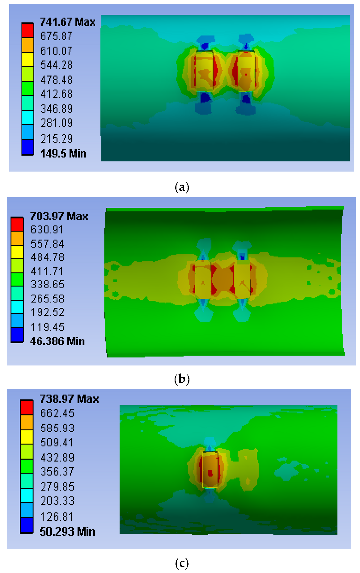
With the help of ANSYS Workbench software, geometric factors such as the defect depth, defect length, and defect spacing changed, respectively; the failure pressure is calculated by applying the form of loading steps and then the critical distance is calculated. The stress nephogram of the different double defect pipe models is shown in Figure 4. It can be concluded that, for the three models, the equivalent stress is divided into two areas: the area close to the defect and the area far away from the defect. In the area close to the defect, the stress distribution is relatively complex and the maximum stress occurs, which conforms to the characteristics of bending stress caused by transverse force and bending moment and belongs to the dangerous area; in the area far away from the defect, the stress is uniformly distributed, which conforms to the characteristics of membrane stress, and belongs to the safe area.

3.2. Impact of Defect Depth on the Critical Distance

The method of control variables is used for this study. For the three double defect pipe models based on the exterior wall, the interior wall, and the interior and exterior wall, the defect length b is calculated by using the formula b = (Rt)^0.5, and the defect width is obtained by deflecting the line between the top vertex and the center of the circle as the coordinate axis by 15° to the left and right sides. The left defect depth a1/t and the right defect depth a2/t are 0.4, 0.45, 0.5, 0.55, and 0.6, respectively. Using the judgment criteria and the critical distance calculation method in Section 2.6 the impact of the defect depth a1/t and a2/t on the critical distance of the double defect pipe models based on the exterior wall, the interior wall, and the interior and exterior wall can be obtained, as shown in Figure 5. It can be concluded that the defect depth a1/t and a2/t vary from 0.4 to 0.6 for the different types of double defect pipe models, and the critical distance varies from 65 to 193 mm for the double defect pipe model based on the exterior wall; for the double defect pipe model based on the interior wall, the critical distance varies from 47.5 to 183 mm; for the double defect pipe model based on the interior and exterior wall, the critical distance varies from 40 to 178 mm; and the critical distance of different types of double defect pipe models increases with the increase in the defect depth.

3.3. Impact of Defect Length on the Critical Distance

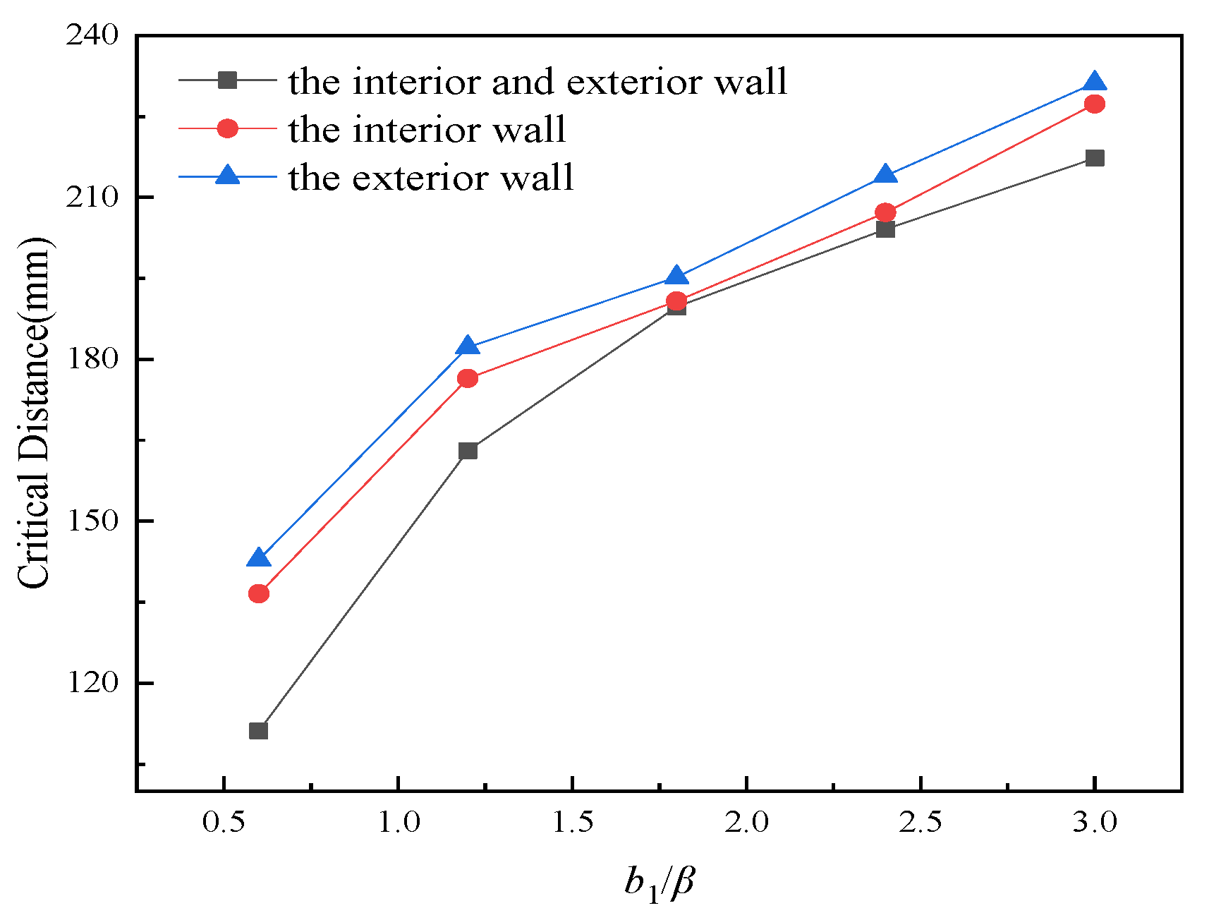
In view of the impact of defect length on the critical distance under the three double defect pipe models based on the exterior wall, the interior wall, and the interior and exterior wall, it is assumed that the defect depth on the two sides of the three double defect pipe models is a/t = 0.5, that is, the defect depth is 10 mm; the defect width is obtained by taking the line between the top vertex of the pipe and the center of the circle as the coordinate axis to deflect 15° on the two sides; the left defect length b1/β and the right defect length b2/β are 0.6, 1.2, 1.8, 2.4, and 3.0, respectively, and β = (Rt)^0.5 = 80 mm. Using the judgment criteria and the critical distance calculation method in Section 2.6, the impact of defect length b1/β and b2/β on the critical distance of the double defect pipe models based on the exterior wall, the interior wall, and the interior and exterior wall can be obtained, as shown in Figure 6. It can be concluded that the defect lengths b1/β and b2/β vary from 0.6 to 3 for the different types of double defect pipe models, and the critical distance varies from 124 to 247.5 mm for the double defect pipe model based on the exterior wall; for the double defect pipe model based on the interior wall, the critical distance varies from 111 to 243.5 mm; for the double defect pipe model based on the interior and exterior wall, the critical distance varies from 81 to 232.5 mm; and the critical distance of the different types of double defect pipe models increases with the increase in defect length, but its growth rate gradually decreases.
For the impact of defect length, the three models also show that when the defect length increases, the critical distance grows, but the growth rate gradually tends to be flat, which is different from defect depth; when the defect length increases, the failure pressure decreases, but its decreasing speed is relatively slow.

3.4. Critical Distance Fitting Formula of Different Types of Double Defect Pipe Models

The dimensionless parameters M1 = a1/t, M2 = a2/t, N1 = b1/β, N2 = b2/β are introduced in the establishment of the function; using MATLAB software, the formula of polynomial function for the critical distance of the three double defect pipe models based on the exterior wall, the interior wall, and the interior and exterior wall is established as follows, and fit:
Llim = c1M13 + c2M12 + c3M1 + c4M23 + c5M22 + c6M2 + c7N13 + c8N12 + c9N1 + c10N23 + c11N22 + c12N2 + c13
where Llim is the critical distance of the double defect pipe models based on the exterior wall, the interior wall, and the interior and exterior wall, mm; c1-c13 are undetermined parameters of the polynomial; M1 is the dimensionless parameter of the defect depth on the left side of the double defect pipe models based on the exterior wall, the interior wall, and the interior and exterior wall; M2 is the dimensionless parameter of the defect depth on the right side of the double defect pipe models based on the exterior wall, the interior wall, and the interior and exterior wall; N1 is a dimensionless parameter of the defect length on the left side of the double defect pipe models based on the exterior wall, the interior wall, and the interior and exterior wall; N2 is a dimensionless parameter of the defect length on the right side of the double defect pipe models based on the exterior wall, the interior wall, and the interior and exterior wall.
Based on 150 sets of critical distance data obtained from different types of double defect pipe models in Section 3.2 and Section 3.3, the regression function in the MATLAB software is used for the fitting, and the critical distance fitting formulas of different types of double defect pipe models are obtained as follows:
For the double defect pipe model based on the exterior wall,
Llim = fM1 + fN1 + fM2 + fN2 − 327.8239
fM1 = 1010.0170M13 − 2378.8767M12 + 2003.6000M1
fM2 = −2982.3355M23 + 3839.5536M22 − 1324.3389M2
fN1 = −4.0200N13 + 17.4092N12 + 18.2857N1
fN2 = −8.5298N23 + 49.5147N22 − 63.7467N
For the double defect pipe model based on the interior wall,
Llim = fM1 + fN1 + fM2 + fN2 − 317.5405
fM1 = −2414.5138M13 + 2579.2806M12 − 490.0823M1
fM2 = 401.7664M23 − 1027.7096M22 + 999.3139M2
fN1 = −7.9146N13 + 37.7637N12 − 8.0452N1
fN2 = −10.3097N23 + 55.2761N22 − 62.4469N2
For the double defect pipe model based on the interior and exterior wall,
Llim = fM1 + fN1 + fM2 + fN2 + 452.3709
fM1 = −3547.8828M13 + 4359.6350M12 − 1258.5208M1
fM2 = −4902.2457M23 + 7282.7058M22 − 3215.4372M2
fN1 = −7.9146N13 + 37.7637N12 − 8.0452N1
fN2 = −10.3102N23 + 53.1496N22 − 50.3494N2
where the parameter fM1 represents the impact of the defect depth on the critical distance on the left side of the double defect pipe models based on the exterior wall, the interior wall, and the interior and exterior wall; the parameter fM2 represents the impact of the defect depth on the critical distance on the right side of the double defect pipe models based on the exterior wall, the interior wall, and the interior and exterior wall; the parameter fN1 represents the impact of the defect length on the critical distance on the left side of the double defect pipe models based on the exterior wall, the interior wall, and the interior and exterior wall; the parameter fN2 represents the impact of the defect length on the critical distance on the right side of the double defect pipe models based on the exterior wall, the interior wall, and the interior and exterior wall.
The critical distance regression fitting curve of different types of double defect pipe models is shown in Figure 7.
For the parameters c1-c13 in the critical distance fitting formula model of different types of double defect pipe model, the sum of squares (R2) and the mean square error (RMSE) are calculated, respectively, to verify its precision: for the double defect pipe model based on the exterior wall, R2 = 0.9755 and RMSE = 7.2750; for the double defect pipe model based on the interior wall, R2 = 0.9634 and RMSE = 9.9727; for the double defect pipe model based on the interior and exterior wall, R2 = 0.9579 and RMSE = 11.4171. It can be concluded that, for the parameters c1-c13 in the critical distance fitting formula of different types of double defect pipe models, the R2 approaches one, which shows that most of the data obtained exists in the fitting curve, and the fitted formula model can accurately reflect the relationship between the critical distance and the geometric elements of the double defect pipe model based on the interior and exterior wall.
By fitting the critical distance formula of the three models, the multiple function formula of the defect depth and the defect length under different defect location distributions is obtained, which can quickly determine whether interference occurs in practical application.

3.5. Comparative Analysis of Defect Interaction in Different Types of Double Defect Models

3.5.1. Comparative Analysis of the Critical Distance of Defect Depth

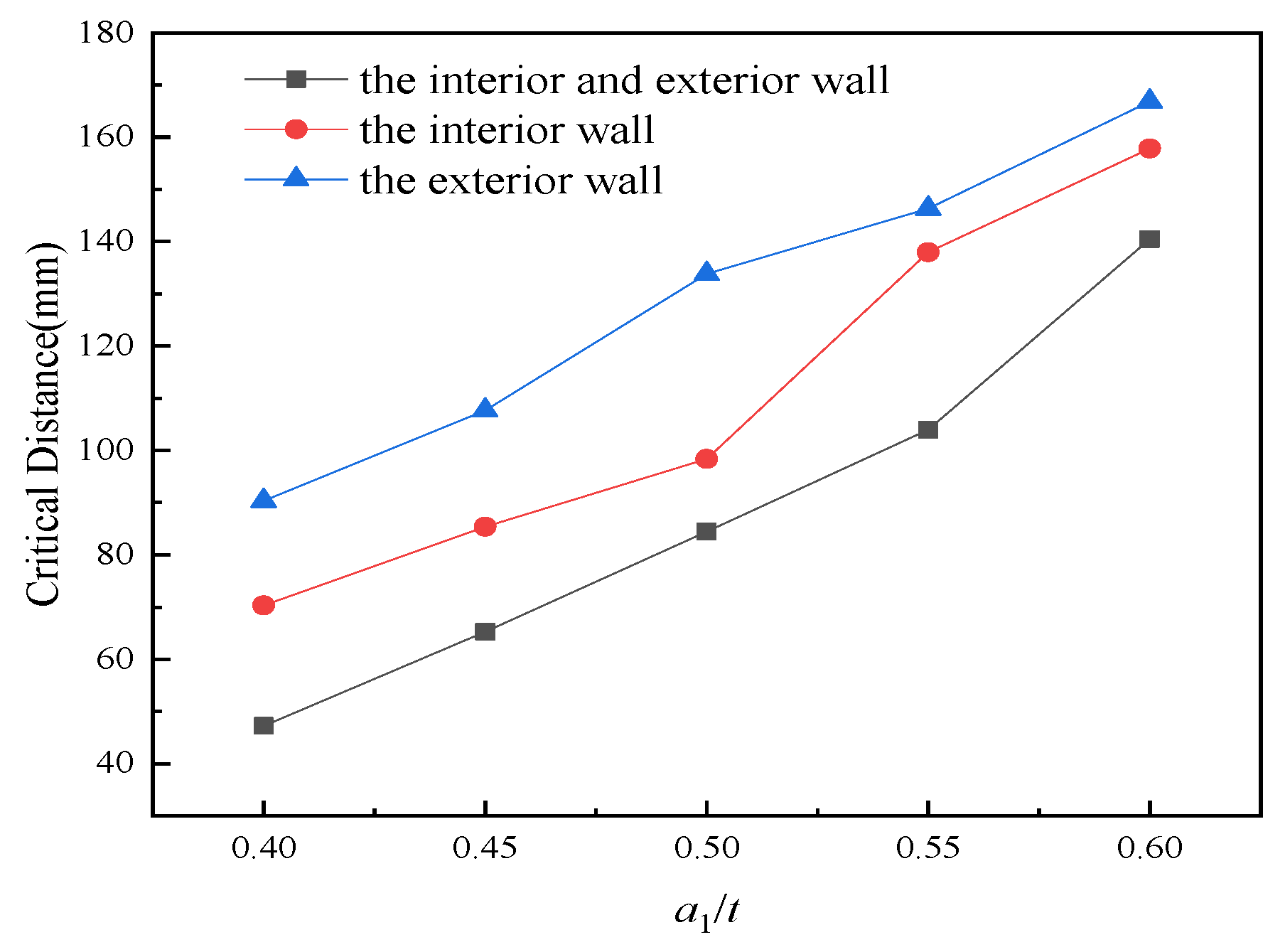
Five groups are randomly selected from the data of the critical distance of the defect length of the three double defect pipe models based on the exterior wall, the interior wall, and the interior and exterior wall. To facilitate observation and comparison, the defect depth of each type a2/t is 0.5; a1/t is 0.4, 0.45, 0.5, 0.55, 0.6; and the defect length b is 80 mm. The defect width is the width displayed after 15° deflection of the left and right sides of the axis of symmetry of the pipe vertex as the center line, a total of 15 sets of data, and the comparative analysis of the critical distance of defect depth of different types of double defect pipe models is shown in Figure 8. It can be concluded that when the defect depth increases, the critical distance grows, whether it is the double defect pipe models based on the exterior wall, the interior wall, or the interior and exterior wall; under the same defect depth, the critical distance of the double defect pipe model based on the exterior wall is the largest, the critical distance of the double defect pipe model based on the interior wall is the second largest, and the critical distance of double defect pipe model based on the interior wall is the smallest; from the growth rate in the figure, the growth rate of the pipe model based on the interior and exterior wall is the largest, the double defect pipe model based on the interior wall takes the second place, and the double defect pipe model based on the exterior wall is the most gentle.

3.5.2. Comparative Analysis of the Critical Distance of Defect Lengths

Five groups are randomly selected from the data of the critical distance of the defect length of the three double defect pipe models based on the exterior wall, the interior wall, and the interior and exterior wall. To facilitate observation and comparison, the defect length b2/β of each type is 1.8; b1/β is 0.6, 1.2, 1.8, 2.4, and 3; and the defect depth a/t is 0.5 (that is, the depth is 10 mm). The defect width is the width of the defect displayed after the left and right deflections of 15°, with the axis of symmetry of the pipe vertex as the centerline. A total of 15 sets of data, and the comparative analysis of the critical distance of the defect length of different types of double defect pipe models, are shown in Figure 9. It can be concluded that when the defect length increases, the critical distance grows, whether it is the double defect pipe models based on the exterior wall, the interior wall, or the interior and exterior wall; under the same defect length, the critical distance of the length of the double defect pipe model based on the exterior wall is the largest, the second largest is the interior wall, and the shortest is the interior and exterior wall; from the growth rate of the broken line, the growth rate of the double defect pipe model based on the interior and exterior wall to the double defect pipe model based on the interior wall and then to the double defect pipe model based on the exterior wall is gradually flat.
Through a comparison extracted from three groups of models under the same defect depth and defect length, it can be concluded that the critical distance of the same defect depth and the same defect length is the double defect pipe model based on the exterior wall > the double defect pipe model based on the interior wall > the double defect pipe model based on the interior and exterior wall. The bearing capacity of the corresponding failure pressure is the double defect pipe model based on the interior and exterior wall, which is > the double defect pipe model based on the interior wall, which is > the double defect pipe model based on the exterior wall. Whether in the same defect depth or in the same defect length, the growth rate of the critical distance of the interior and exterior wall is greater than that of the double defect pipe model based on the interior wall and the double defect pipe model based on the exterior wall, and the corresponding rate of the reduction in the bearing capacity of the failure pressure is also faster than that of the double defect pipe model based on the interior wall and the double defect pipe model based on the exterior wall.

3.6. Applicability Analysis of the Critical Distance Fitting Formula for Different Pipe Models

3.6.1. Conservative Analysis of the Three Models

The critical distance ratio K is introduced to investigate the conservatism of the three double defect pipe models based on the exterior wall, the interior wall, and the interior and exterior wall. Where the critical distance ratio K is:
K = calculated critical distance/actual critical distance
When K < 1, the calculated critical distance is less than the actual critical distance, and the calculated result is too conservative; when K = 1, the calculated critical distance is equal to the actual critical distance, which is the most ideal prediction form; when K > 1, the calculated critical distance is greater than the actual critical distance, and the calculated result is too radical and not reliable.
By calculating the critical distance ratio K of 50 sets of data for each of the three double defect pipe models based on the exterior wall, the interior wall, and the interior and exterior wall, the critical distance analysis diagram is obtained as shown in Figure 10. It can be concluded that the critical distance ratio K of the double defect pipe model based on the exterior wall fluctuates between 0.9 and 1.25, the critical distance ratio K of the double defect pipe model based on the interior wall fluctuates between 0.8 and 1.25, and the critical distance ratio K of the double defect pipe model based on the interior and exterior wall fluctuates between 0.5 and 1.3. For the double defect pipe model based on the exterior wall, the critical distance ratio K is mostly between 0.95 and 1.05, and the results are relatively ideal; for the double defect pipe model based on the interior wall, the critical distance ratio K is mostly between 0.9 and 1.05, and the results are relatively ideal; for the double defect pipe model based on the interior and exterior wall, the critical distance ratio K is mostly between 0.95 and 1.0, and the result is the most ideal, compared with the other two interior wall models. The number of data points whose critical distance ratio K is greater than 1 through the statistical analysis of three models is 29 data points for the double defect pipe model based on the exterior wall, 26 data points for the double defect pipe model based on the interior wall, and 24 data points for the double defect pipe model based on the interior and exterior wall. If conservatism is strictly judged according to the number of critical distance ratios K greater than one, the double defect pipe model based on the exterior wall is the most conservative, the double defect pipe model based on the interior wall is more conservative, and the double defect pipe model based on the interior and exterior wall is more radical. If the data are segmented, for the double defect pipe model based on the exterior wall, the data are relatively dense and the fluctuation range is small from the perspective of the whole, so segmentation analysis is not needed, and it is slightly conservative from the perspective of the whole; for the double defect pipe model based on the interior wall, the first 17 data points are used as the first half, and the last 33 data points are used as the second half. By observing the first half section, it can be concluded that the data are relatively scattered and fluctuate greatly, which is slightly radical. However, through the observation of the second half section, the data are less dense and fluctuate less, which is relatively conservative, and considering the overall conservativeness, it is slightly conservative. For the double defect pipe model based on the interior and exterior wall, it is divided into 3 sections; the first 18 data points are the 1st section, the 19th to 31st data points are the 2nd section, and the 32nd to 50th data points are the 3rd section. The first section has a high dispersion of data, a large fluctuation range, and a more radical result. The second section has a centralized distribution of data, a small fluctuation range, and is a little conservative. The third section is more dispersed than the second section, more concentrated than the first section, and the fluctuation range is between the first section and the second section; however, from the perspective of whether it changes around one, the gap is obvious and slightly radical. From the perspective of the proportion of conservative and radical, radical accounts for the majority. Therefore, under comprehensive consideration, the double defect pipe model based on the interior and exterior wall is slightly radical. From a precise point of view, the probability that the critical distance ratio K of the three models exists between 0.95 and 1.05 is statistically calculated. The probability of the critical distance ratio K of the double defect pipe model based on the exterior wall, the double defect pipe model based on the interior wall, and the double defect pipe model based on the interior and exterior wall within the range of 0.95 to 1.05 are 72%, 58%, and 46%, respectively. It can be concluded that the double defect pipe model based on the exterior wall is more reasonable, the double defect pipe model based on the interior wall is second, and the double defect pipe model based on the interior and exterior wall is low.
In summary, the calculation results of the double defect pipe model based on the exterior wall are conservative, the calculation results of the double defect pipe model based on the interior wall are conservative, and the calculation results of the double defect pipe model based on the interior and exterior wall are more radical. Through the analysis and calculation of 150 sets of data from the 3models, the critical distance ratio K is introduced for conservative analysis. Through the calculation of the K value, it can be found that most of the introduced K values fluctuate around one, so it is ideal to use the critical distance ratio for conservative analysis. The three models are excellent in the critical distance ratio. After comprehensive consideration, the double defect pipe model based on the exterior wall is conservative, the double defect pipe model based on the interior wall is conservative, and the double defect pipe model based on the interior and exterior wall is more radical.

3.6.2. Error Analysis of the Three Models

The relative error is introduced to examine the accuracy of the three double defect pipe models based on the exterior wall, the interior wall, and the interior and exterior wall. The relative error is as follows:
Relative error = (actual critical distance − calculated critical distance)/actual critical distance
We calculated the error according to the above definition formula. When the relative error is positive, the actual critical distance is greater than the calculated critical distance, which means that the critical distance is more conservative than the K result, and the larger the relative error value, the more conservative the error is; when the relative error is negative, the actual critical distance is less than the calculated critical distance, which means that the critical distance is more radical than the K result, and the larger the relative error of the negative value, the more radical the error is. Therefore, if the relative error fluctuates around zero, it is ideal and the smaller the fluctuation range is, the more ideal it is.
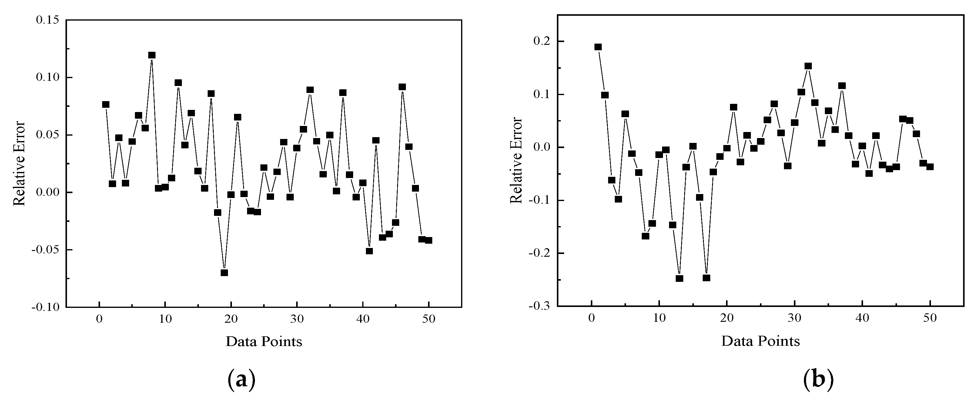
By calculating the relative error of 50 sets of data for each of the 3 double defect pipe models based on the exterior wall, the interior wall, and the interior and exterior wall, the relative error analysis diagram was obtained as shown in Figure 11. It can be concluded that, in general, the relative error of the double defect pipe model based on the interior and exterior wall is the largest, the double defect pipe model based on the interior wall is the second largest, and the double defect pipe model based on the exterior wall is the smallest. From the data distribution, the relative error of the double defect pipe model based on the exterior wall is mostly between −0.05 and 0.05, the relative error of the double defect pipe model based on the interior wall is mostly between −0.1 and 0.1, and the relative error of the double defect pipe model based on the interior and exterior wall is mostly between −0.1 and 0.05. From the centralized distribution of the relative error data of the three models, the relative error of the double defect pipe model based on the exterior wall is the smallest, the double defect pipe model based on the interior and exterior wall takes the second place, and the double defect pipe model based on the interior wall has the largest relative error. From the perspective of accuracy, the accuracy is high when the relative error is between −0.05 and 0.05. The overall accuracy can be judged by examining the probability that the relative error occurs in this range. Since the probability of the relative error of the double defect pipe models based on the exterior wall, the interior wall, and the interior and exterior wall between −0.05 and 0.05 are 72%, 58%, and 46%, respectively, the overall relative error of the double defect pipe model based on the exterior wall is small and the results are the most accurate. The overall relative error of the double defect pipe model based on the interior wall is relatively large and the results are relatively accurate; the overall relative error of the double defect pipe model based on the interior and exterior wall is the largest and the accuracy of the results is low. If the data are segmented, for the double defect pipe model based on the exterior wall, the data concentration is good, the fluctuation range is small, the relative error is small, and the accuracy is high. For the double defect pipe model based on the interior wall, it can be divided into 4 sections: the 1st 17 data points are the 1st section, which has a large fluctuation range and a large relative error; the 18th to 30th data points are the 2ndsection, which has a small fluctuation range and a small relative error; the 31st to 38th data points are the 3rd section, which has a large fluctuation range and the relative error is said to be large; the 39th to 50th data points are the 4th section, which has basically no fluctuation, a high concentration, and a small relative error. From the comprehensive overall analysis, the relative error is obviously large and the precision is poor. For the double defect pipe model based on the interior and exterior wall, it can be divided into 3 sections: the 1st 18 data points are the 1st section, which has high data dispersion, poor concentration, and large relative error; the 19th to 31st data points are the 2nd section, which has a high data concentration and small relative error; the 32nd to 50th data points are the 3rd section, which has high data dispersion and poor concentration, so the relative error is large and the accuracy is poor.
In order to analyze the error more intuitively and effectively, the mean absolute error and the mean relative error are introduced. The mean absolute error is the average value of the actual critical distance minus the absolute value of the calculated critical distance in the 50 groups of data of the 3 double defect pipe models based on the exterior wall, the interior wall, and the interior and exterior wall. The mean relative error is the average value of the relative error in the 50 groups of data of the 3 double defect pipe models based on the exterior wall, the interior wall, and the interior and exterior wall. The mean absolute error and the mean relative error of the three models of the exterior wall, the interior wall, and the interior and exterior wall pipes with double defects are shown in Table 4. From Table 4, we can see that the mean relative error of the three models is negative, but is very close to zero, and the fitting calculation data are relatively ideal. If we only consider the positive and negative values, we can see that their values are negative and the corresponding critical distance is more radical than the K result; for the mean absolute error, its value is of the order of the exterior double defect pipe model, the interior double defect pipe model, and the interior and exterior double defect pipe model, and the mean absolute error of the 3 models is below 0.1, while the mean absolute error of the exterior double defect pipe model is the smallest, indicating that the exterior double defect pipe model performs best in the error analysis of the critical distance ratio K. By comparing the mean absolute error of the three models, it can be concluded that the double defect pipe model based on the exterior wall performs best under the critical distance ratio K.
Through the introduction of relative error, mean absolute error, and mean relative error, it can be concluded that the calculated critical distance of the three model formulas has little difference with the actual critical distance. The double defect pipe model based on the exterior wall is the most outstanding in the error analysis of the critical distance ratio K, the double defect pipe model based on the interior wall takes the second place, and the double defect pipe model based on the interior wall is the worst.

4. Conclusions

For the three double defect pipe models based on the exterior wall, the interior wall, and the interior and exterior wall, the equivalent stress is divided into two areas: area close to the defect and area far away from the defect.
By introducing the blasting experimental data, the established finite element model has a high accuracy and can well predict the failure pressure of the pipeline with defects. For the three double defect pipe models, the critical distance and growth rate will increase with the increase in defect depth. With the increase in defect length, the critical distance increases, but the growth rate gradually tends to be flat, which is different from the impact of defect depth. Through the formula fitting of the critical distance of the three double defect pipe models, the multiple function formula of the defect depth and the defect length is obtained under different defect location distributions with high precision.
Through the calculation of the K value, it can be found that most of the introduced K values fluctuate around one, so it is ideal to use the critical distance ratio for the conservative analysis. The three models are excellent in the critical distance ratio. After comprehensive consideration, the double defect pipe model based on the exterior wall is conservative, the double defect pipe model based on the interior wall is conservative, and the double defect pipe model based on the interior and exterior wall is more radical.

Author Contributions

Conceptualization, Z.W. and X.L.; methodology, Z.W., M.L. and X.L.; investigation, Z.W. and M.L.; resources, Z.W. and Z.Z.; writing—original draft preparation, Z.W. and M.L.; writing—review and editing, Z.W., X.L. and Z.Z.; visualization, M.L.; supervision, X.L. and Z.Z.; funding acquisition, Z.W. and Z.Z. All authors have read and agreed to the published version of the manuscript.

Funding

This research was funded by the National Natural Science Foundation of China (21763030, 52076196) and Key Research; Development Program of Zhejiang Province (2021C05006); Innovation Capacity Support Plan in Shanxi Province of China (2020TD-032); Science and Technology Department Project in Shanxi Province of China (2022GY-145).

Institutional Review Board Statement

Not applicable.

Informed Consent Statement

Not applicable.

Data Availability Statement

Not applicable.

Conflicts of Interest

The authors declare no conflict of interest.

References

  1. Wang, Y.; Wharton, J.A.; Shenoi, R.A. Mechano-electrochemical modelling of corroded steel structures. Eng. Struct. 2016, 128, 1–14. [Google Scholar] [CrossRef] [Green Version]
  2. Srikanth, S.; Sankaranarayanan, T.S.N.; Gopalakrishna, K.; Narasimhan, B.R.V.; Das, T.V.K.; Das, S.K. Corrosion in a buried pressurised water pipeline. Eng. Fail. Anal. 2005, 12, 634–651. [Google Scholar] [CrossRef]
  3. Cosham, A.; Hopkins, P.; Macdonald, K.A. Best practice for the assessment of defects in pipelines-Corrosion. Eng. Fail. Anal. 2007, 14, 1245–1265. [Google Scholar] [CrossRef]
  4. Saeedikhani, M.; Blackwood, D.J. Finite element method for thin film corrosion modelling: Where we advanced and where we would like to advance. Corros. Mater. Degrad. 2020, 1, 273–281. [Google Scholar] [CrossRef]
  5. Moustabchir, H.; Azari, Z.; Hariri, S.; Dmytrakh, I. Experimental and numerical study of stress–strain state of pressurized cylindrical shells with external defects. Eng. Fail. Anal. 2010, 17, 506–514. [Google Scholar] [CrossRef]
  6. Moustabchir, H.; Arbaoui, J.; Azari, Z.; Hariri, S.; Pruncu, C.I. Experimental/numerical investigation of mechanical behaviour of internally pressurized cylindrical shells with external longitudinal and circumferential semi-elliptical defects. Alex. Eng. J. 2017, 57, 1339–1347. [Google Scholar] [CrossRef]
  7. Fekete, G.; Varga, L. The effect of the width to length ratios of corrosion defects on the burst pressures of transmission pipelines. Eng. Fail. Anal. 2012, 21, 21–30. [Google Scholar] [CrossRef]
  8. Duane, S.C.; Roy, J.P. Prediction of the failure pressure for complex corrosion defects. Int. J. Press. Ves. Pip. 2002, 79, 279–287. [Google Scholar]
  9. Hosseini, A.; Cronin, D.; Plumtree, A. Crack in corrosion defect assessment in transmission pipelines. J. Press. Vessel. Technol. 2013, 135, 8. [Google Scholar] [CrossRef]
  10. Ma, B.; Shuai, J.; Liu, D.X.; Xu, K. Assessment on failure pressure of high strength pipeline with corrosion defects. Eng. Fail. Anal. 2013, 32, 209–219. [Google Scholar] [CrossRef]
  11. Sun, M.M.; Li, X.; Liu, J.K. Determination of folias factor for failure pressure of corroded pipeline. J. Press. Vessel. Technol. 2020, 142, 31802. [Google Scholar] [CrossRef]
  12. Yeom, K.J.; Lee, Y.K.; Oh, K.H.; Kim, W.S. Integrity assessment of a corroded API X70 pipe with a single defect by burst pressure analysis. Eng. Fail. Anal. 2015, 57, 553–561. [Google Scholar] [CrossRef]
  13. Shuai, Y.; Shuai, J.; Xu, K. Probabilistic analysis of corroded pipelines based on a new failure pressure model. Eng. Fail. Anal. 2017, 81, 216–233. [Google Scholar] [CrossRef]
  14. Mokhtari, M.; Melchers, R.E. A new approach to assess the remaining strength of corroded steel pipes. Eng. Fail. Anal. 2018, 93, 144–156. [Google Scholar] [CrossRef]
  15. Majid, Z.A.; Mohsin, R.; Yusof, M.Z. Experimental and computational failure analysis of natural gas pipe. Eng. Fail. Anal. 2012, 19, 32–42. [Google Scholar] [CrossRef]
  16. Caleyo, F.; González, J.L.; Hallen, J.M. A study on the reliability assessment methodology for pipelines with active corrosion defects. Int. J. Press. Ves. Pip. 2002, 79, 77–86. [Google Scholar] [CrossRef]
  17. Cerit, M.; Genel, K.; Eksi, S. Numerical investigation on stress concentration of corrosion pit. Eng. Fail. Anal. 2009, 16, 2467–2472. [Google Scholar] [CrossRef]
  18. Cerit, M. Numerical investigation on torsional stress concentration factor at the semielliptical corrosion pit. Corros. Sci. 2013, 67, 225–232. [Google Scholar] [CrossRef]
  19. Xu, L.Y.; Cheng, Y.F. Reliability and failure pressure prediction of various grades of pipeline steel in the presence of corrosion defects and pre-strain. Int. J. Press. Ves. Pip. 2012, 89, 75–84. [Google Scholar] [CrossRef]
  20. Xu, L.Y.; Cheng, Y.F. Development of a finite element model for simulation and prediction of mechanoelectrochemical effect of pipeline corrosion. Corros. Sci. 2013, 73, 150–160. [Google Scholar] [CrossRef]
  21. Zelmati, D.; Ghelloudj, O.; Amirat, A. Correlation between defect depth and defect length through a reliability index when evaluating of the remaining life of steel pipeline under corrosion and crack defects. Eng. Fail. Anal. 2017, 79, 171–185. [Google Scholar] [CrossRef]
  22. Chouchaoui, B.A.; Pick, R.J. Behaviour of circumferentially aligned corrosion pits. Int. J. Press. Ves. Pip. 1994, 57, 187–200. [Google Scholar] [CrossRef]
  23. Chouchaoui, B.A.; Pick, R.J. Behaviour of longitudinally aligned corrosion pits. Int. J. Press. Ves. Pip. 1996, 67, 17–35. [Google Scholar] [CrossRef]
  24. Benjamin, A.C.; Freire, J.L.F.; Vieira, R.D.; Cunha, D.J.S. Interaction of corrosion defects in pipelines-Part 1: Fundamentals. Int. J. Press. Ves. Pip. 2016, 144, 56–62. [Google Scholar] [CrossRef]
  25. Benjamin, A.C.; Freire, J.L.F.; Vieira, R.D.; Cunha, D.J.S. Interaction of corrosion defects in pipelines-Part 2: MTI JIP database of corroded pipe tests. Int. J. Press. Ves. Pip. 2016, 145, 41–59. [Google Scholar] [CrossRef]
  26. Chen, Y.F.; Zhang, H.; Zhang, J.; Liu, X.B.; Li, X.; Zhou, J. Failure assessment of X80 pipeline with interacting corrosion defects. Eng. Fail. Anal. 2015, 47, 67–76. [Google Scholar] [CrossRef]
  27. Bedairi, B.; Cronin, D.; Hosseini, A.; Plumtree, A. Failure prediction for crack-in-corrosion defects in natural gas transmission pipelines. Int. J. Press. Vessel. Pip. 2012, 6, 90–99. [Google Scholar] [CrossRef]
  28. Al-Owaisi, S.S.; Becker, A.A.; Sun, W. Analysis of shape and location effects of closely spaced metal loss defects in pressurised pipes. Eng. Fail. Anal. 2016, 68, 172–186. [Google Scholar] [CrossRef]
  29. Soares, E.; Bruère, V.M.; Afonso, S.M.B.; Willmersdorf, R.B.; Lyra, P.R.M.; Bouchonneau, N. Structural integrity analysis of pipelines with interacting corrosion defects by multiphysics modeling. Eng. Fail. Anal. 2019, 97, 91–102. [Google Scholar] [CrossRef]
  30. Sun, J.L.; Cheng, Y.F. Assessment by finite element modeling of the interaction of multiple corrosion defects and the effect on failure pressure of corroded pipelines. Eng. Struct. 2018, 165, 278–286. [Google Scholar] [CrossRef]
  31. Sun, J.L.; Cheng, Y.F. Investigation by numerical modeling of the mechano-electrochemical interaction of circumferentially aligned corrosion defects on pipelines. Thin-Walled. Struct. 2019, 144, 106314. [Google Scholar] [CrossRef]
  32. Sun, M.M.; Zhao, H.S.; Li, X.; Liu, J.K.; Xu, Z.G. A new evaluation method for burst pressure of pipeline with colonies of circumferentially aligned defects. Ocean. Eng. 2021, 222, 108628. [Google Scholar] [CrossRef]
  33. Al-Owaisi, S.; Becker, A.A.; Sun, W.; Al-Shabibi, A.; Al-Maharbi, M.; Pervez, T.; Al-Salmi, H. An experimental investigation of the effect of defect shape and orientation on the burst pressure of pressurised pipes. Eng. Fail. Anal. 2018, 93, 200–213. [Google Scholar] [CrossRef]
  34. Chen, Y.F.; Zhang, H.; Zhang, J.; Li, X.; Zhou, J. Failure analysis of high strength pipeline with single and multiple corrosions. Mater. Design. 2015, 67, 552–557. [Google Scholar] [CrossRef]
  35. Lo, M.; Karuppanan, S.; Ovinis, M. Failure pressure prediction of a corroded pipeline with longitudinally interacting corrosion defects subjected to combined loadings using FEM and ANN. J. Mar. Sci. Eng. 2021, 9, 281. [Google Scholar] [CrossRef]
  36. Chen, Y.F.; Li, X.; Zhou, J.; Guan, J. Study on interaction relationship for submarine pipeline with axial corrosion defects. China Ocean. Eng. 2008, 22, 359–370. [Google Scholar]
  37. Li, X.; Bai, Y.; Su, C.L.; Li, M.S. Effect of interaction between corrosion defects on failure pressure of thin wall steel pipeline. Int. J. Press. Ves. Pip. 2016, 138, 8–18. [Google Scholar] [CrossRef]
  38. Huang, K.; Yang, L.; Li, A.R. Study on the influencing factors of interference effect of corrosion defects on the inner and outer walls of oil and gas pipelines. Surf. Tech. 2020, 49, 199–204. [Google Scholar]
  39. Freire, J.L.F.; Vieira, R.D.; Benjamin, A.C. PAR T 1: Experimental techniques in the field of pipeline integrity. Exp. Tech. 2006, 30, 44–50. [Google Scholar] [CrossRef]
  40. Freire, J.L.F.; Vieira, R.D.; Castro, J.T.P.; Benjamin, A.C. PART 3: Burst tests of pipeline with extensive longitudinal metal loss. Exp. Tech. 2006, 30, 60–65. [Google Scholar] [CrossRef]
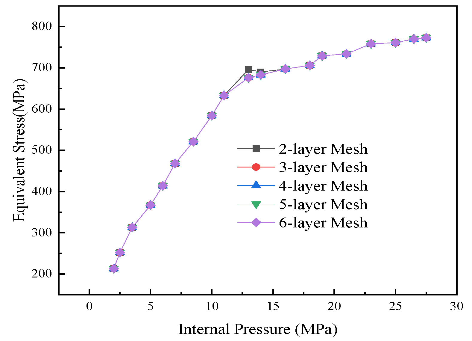
Figure 1. Sensitivity of the mesh.
Jmse 11 00502 g001
Figure 2. Example of the critical distance calculation.
Jmse 11 00502 g002
Figure 3. Geometric model of different types of double defects: (a) the exterior wall; (b) the interior wall; (c) the interior and exterior walls.
Jmse 11 00502 g003aJmse 11 00502 g003b
Figure 4. Stress nephogram of different double defect pipe models: (a) the exterior wall; (b) the interior wall; (c) the interior and exterior wall.
Jmse 11 00502 g004
Figure 5. Diagram of impact of defect depth on the critical distance: (a) the exterior wall; (b) the interior wall; (c) the interior and exterior wall.
Jmse 11 00502 g005
Figure 6. Diagram of impact of defect length on the critical distance: (a) the exterior wall; (b) the interior wall; (c) the interior and exterior wall.
Jmse 11 00502 g006
Figure 7. Critical distance regression fitting curve of different pipe models: (a) the exterior wall; (b) the interior wall; (c) the interior and exterior wall.
Jmse 11 00502 g007
Figure 8. Comparative analysis of the critical distance of defect depth.
Jmse 11 00502 g008
Figure 9. Comparative analysis of the critical distance of defect length.
Jmse 11 00502 g009
Figure 10. Critical distance ratio K of the three models: (a) the exterior wall; (b) the interior wall; (c) the interior and exterior wall.
Jmse 11 00502 g010
Figure 11. Relative error analysis of the three models: (a) the exterior wall; (b) the interior wall; (c) the interior and exterior wall.
Jmse 11 00502 g011aJmse 11 00502 g011b
Table 1. Parameters of the pipe section model.
MaterialYield Strength (MPa)Tensile Strength (MPa)Modulus of Elasticity (GPa)Poisson’s Ratio
X1006907602100.3
Table 2. Geometric parameters and FEM failure pressure of the X100 pipeline.
NumberD (mm)t (mm)a (mm)b (mm)Burst Pressure (MPa)FEM (MPa)
1132022.911.5111015.414.5
2132022.911.510131514.2
3132022.911.460918.116.5
Table 3. Example of the calculation of the critical influence factor.
Defect Spacing (mm)Pd (MPa)Ps (MPa)Critical Influence Factor ω (%)
8024.0326.279.32
12024.5926.276.85
16025.0926.274.69
20025.4226.273.35
24025.7126.272.15
Table 4. Error analysis table of the three models.
Model CategoryMean Relative ErrorMean Absolute Error
exterior wall−0.00290.0373
interior wall−0.00590.0625
interior and exterior wall−0.00800.0864
Disclaimer/Publisher’s Note: The statements, opinions and data contained in all publications are solely those of the individual author(s) and contributor(s) and not of MDPI and/or the editor(s). MDPI and/or the editor(s) disclaim responsibility for any injury to people or property resulting from any ideas, methods, instructions or products referred to in the content.