Coupled Translational–Rotational Stability Analysis of a Submersible Ocean Current Converter Platform Mooring System under Typhoon Wave

Abstract

This study proposes a mathematical model for the coupled translational–rotational motions of a mooring system for an ocean energy converter working under a typhoon wave impact. The ocean energy convertor comprises two turbine generators and an integration structure. The configuration of the turbine blade and the floating platform is designed. The two turbine blades rotate reversely at the same rotating speed for rotational balance. If the current velocity is 1.6 m/s and the tip speed ratio is 3.5, the power generation is approximately 400 kW. In the translational and rotational motions of elements under ocean velocity, the hydrodynamic parameters in the fluid–structure interaction are studied. Initially, the hydrodynamic forces and moments on the converter and the platform are calculated and further utilized in obtaining the hydrodynamic damping and stiffness parameters. The 18 degrees of freedom governing equations of the mooring system are derived. The solution method of the governing equations is utilized to determine the component’s motion and the ropes’ dynamic tensions. In the mooring system, the converter is mounted under a water surface at some safe depth so that it can remain undamaged and stably generate electricity under typhoon wave impact and water pressure. It is theoretically verified that the translational and angular displacements of the converter can be kept small under the large wave impact. In other words, the water pressure on the converter cannot exceed the predicted value. The relative flow velocity of the convertor to the current is kept fixed such that the power efficiency of convertor can be maintained as high. In addition, the dynamic tension of the rope is far less than its breaking strength.

1. Introduction

Ocean current power generation is a potential renewable energy technology. The Taiwan Kuroshio current has a potential capacity of over 4 GW [1]. However, the seabed beneath the Kuroshio current is almost over 1000 m in the area mentioned above. The deep mooring technology is essential for harnessing that energy. Additionally, the typhoon wave impact affects the operation of the ocean power generation system. Hence, there is a need to model and develop a technology overcoming these limitations.

So far, Chen et al. [1] successfully tested the 50-kW ocean current convertor mooring to the 850 m deep seabed in the Taiwan Pingtung sea area. IHI and NEDO [2] tested a 100 kW ocean current convertor mooring to the 100 m deep seabed beneath the Japan Kuroshio current. The current converter generated approximately 30 kW under the current speed of 1.0 m/s. These two experiments were conducted under the small excitation of wave and in a few weeks. The goal of these experiments was to test the power performance of the developed convertors. However, it is for a commercial power farm that the convertor will be safe working for a long time and under different wave impact. Therefore, the deep mooring theory and technology for the ocean current convertor system are in great need of development. Nobel et al. [3] presented the standards and guidance for the development and testing of the devices for marine renewable energy.

Lin et al. [4] investigated the dynamic stability of the mooring system under regular wave and ocean current. The significant effects of some parameters on the dynamical stability of the mooring system were detected. The lightweight high-strength PE (HSPE) mooring rope was determined to be suitable for the deep mooring system. C’atipovic et al. [5] investigated the hydrodynamic damping force of fiber mooring lines taking longitudinal deformation by the finite element method. Lin and Chen [6] developed the linear elastic model for the mooring system with PE mooring rope. They proposed a methodology to protect the convertor from the typhoon wave–current impact. The protection function of the proposed methodology under Typhoon wave impact was theoretically verified. Lin et al. [7] investigated the dynamic stability of the mooring system for surfaced convertor under the regular wave during non-typhoon periods and steady ocean current. Lin et al. [8] proposed a mooring system that enabled the energy convertor to work under typhoon wave impact. The plane translational motion of the mooring system was simulated in the linear elastic model. The concentrated mass assumption was made. Meanwhile, only the hydrodynamic forces of the convertor and platform were considered in the surge motion.

The mathematical model of the mooring system is also important for wave energy converters (WEC). Davidson and Ringwood [9] reviewed the mathematical modeling of mooring systems for wave energy converters. Chen et al. [10] investigated the wave-induced motions of a floating WEC with mooring lines by using the Smoothed Particle Hydrodynamics (SPH) method. Xiang et al. [11] proposed the finite element cable model to study the performance of a buoy mooring system. Paduano et al. [12] validated the quasi-static and dynamic lumped-mass models. Touzon et al. [13] compared a linearized frequency domain model, a non-linear quasistatic time domain model, and a non-linear dynamic model for WEC. Xiang et al. [14] investigated the dynamic response of a floating wind turbine foundation with a Taut Mooring System.

Anagnostopoulos [15] studied the dynamic performance of offshore platforms under wave loadings in the Morison model. It was determined that the effect of hydrodynamic damping on the resonant response of the structure is significant. Bose et al. [16] studied the dynamic stability of an airfoil supported by a spring. The problem of fluid–structure interaction is usually solved by using numerical methods such as the boundary element method [17], the finite volume method [18], the Lagrangian–Eulerian Method [19], the particle-based method [20], and the hybrid methods [21].

Lin et al. [5,6,7] investigated the plane translational motion of the mooring system in the linear elastic model. The concentrated mass assumption was made but the fluid–structure interaction (FSI) was not completely considered. In this study, a mooring system for an ocean energy convertor that is working under the typhoon wave impact is proposed. The mathematical model of the coupled translational–rotational motions of the system is derived. The configuration of the turbine blade and the floating platform is designed. The hydrodynamic forces and moments on the operational convertor and the platform in motion are determined by using the finite volume method. The damping effect of the fluid–structure interaction on the stability of the mooring system under typhoon wave is investigated.

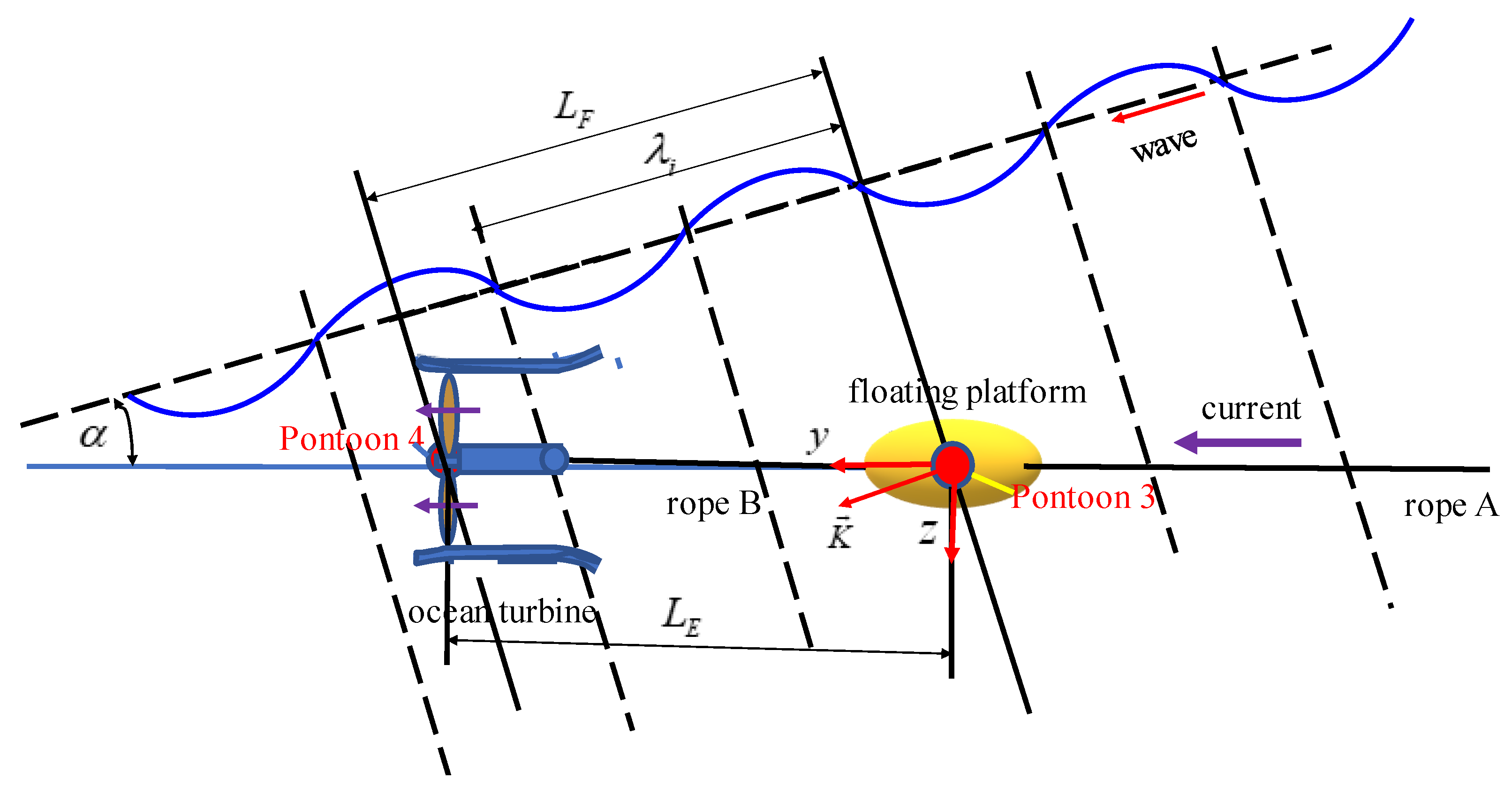
2. Mathematical Model

To avoid the typhoon wave impact, the energy convertor and the floating platform were submerged to a depth of approximately 60 m, as shown in Figure 1. Therefore, the direct impact of the typhoon wave is almost negligible. In this study, the translational–rotational response of the mooring system under coupled wave–ocean effect is investigated. The translational motions include ‘heave’, ‘surge’, and ‘sway’. The rotational motions include ‘pitch’, ‘roll’, and ‘yaw’. The ocean energy convertor is composed of two turbine generators and an integration structure. When ocean currents flow through the energy convertor, the turbine blade rotates and drives the power generator to generate electricity. Meanwhile, the convertor and the floating platform are subjected to the hydrodynamic force and moment due to the ocean current–structure interaction. Lin and Chen [3] determined that the HSPE rope could be assumed as a straight line over a certain amount of ocean current drag force because the force deformation of the HSPE rope was negligible. The linear elastic model proposed by Lin and Chen [3] is used to analyze the motion equation of the overall mooring system.

Based on the facts for ocean current energy converters (OCEC), the following assumptions are made:

−

The current flow is steady.

−

The HSPE mooring ropes are used.

−

Under the ocean velocity, the deformed configuration of the HSPE rope is nearly straight.

−

The elongation strain of the ropes is small.

−

The translational and rotational displacements of the components are small.

−

The tension of the rope is considered uniform.

These displacements of the component and tensions of ropes include (1) the static one under the steady current only, (2) the dynamic one due to the wave impact and current. The global translational and the rotational displacement of the component are expressed as

$$x_i=x_{is}+x_{id},\hspace{1em}{y}_i=y_{is}+y_{id},\hspace{1em}{z}_i=z_{is}+z_{id},\hspace{1em}i=1, 2, 3, 4,$$

$${\phi }_{jx}={\phi }_{jxs}+{\phi }_{jxd}, {\phi }_{jy}={\phi }_{jys}+{\phi }_{jyd}, {\phi }_{jz}={\phi }_{jzs}+{\phi }_{jzd}, j=1,2.$$

(1)

The total tensions of the ropes are expressed as

$$T_i=T_{is}+T_{id},\hspace{1em}i=A, B, C, D.$$

(2)

Static Displacements and Equilibrium under the Steady Current Only

Under the steady current only, the static displacements of the components are obtained:

$$x_0=0,\hspace{1em}\hspace{1em}{y}_0=0,\hspace{1em}\hspace{1em}{z}_0=0,$$

$$x_{1s}=H_{bed}-L_C=L_A\sin {\theta }_{As},\hspace{1em}\hspace{1em}{y}_{1s}=L_A\cos {\theta }_{As},\hspace{1em}\hspace{1em}{z}_{1s}=0,$$

$$x_{2s}=H_{bed}-L_D=x_{1s}-L_B\sin {\theta }_{Bs},\hspace{1em}\hspace{1em}{y}_{2s}=y_{1s}+L_B\cos {\theta }_{Bs},\hspace{1em}\hspace{1em}{z}_{2s}=0,$$

$$x_{3s}=x_{1s}+L_C=H_{bed},\hspace{1em}\hspace{1em}{y}_{3s}=y_{1s},\hspace{1em}\hspace{1em}{z}_{3s}=0,$$

$$x_{4s}=x_{3s}=x_{2s}+L_D=H_{bed},\hspace{1em}\hspace{1em}{y}_{4s}=y_{2s},\hspace{1em}\hspace{1em}{z}_{4s}=0,$$

$${\phi }_{jks}=0, j=1,2; k=x,y,z.$$

(3)

The global setting angle θ_As of rope A is

$$\sin {\theta }_{As}=x_{1s}/L_A.$$

(4)

The global setting angle θ_Bs of rope B is

$$\sin {\theta }_{Bs}=\left(x_{1s}-x_{2s}\right)/L_B.$$

(5)

Under the steady current only, the static equilibrium of the platform in the y-direction is

$$T_{As}\cos {\theta }_{As}-T_{Bs}\cos {\theta }_{Bs}=f_{Pys}=\frac{1}{2}{C}_{DPy}\rho A_{PY}{V}^2.$$

(6)

The static equilibrium of the platform in the x-direction is

$$T_{Cs}+F_{B1s}=T_{As}\sin {\theta }_{As}+T_{Bs}\sin {\theta }_{Bs}+W_1.$$

(7)

The static equilibrium of the energy convertor in the y-direction is

$$T_{Bs}\cos {\theta }_{Bs}=f_{Tys}=C_{DTy}\frac{1}{2}\rho A_{Ty}{V}^2.$$

(8)

The static equilibrium of the energy convertor in the x-direction is

$$F_{B2s}=W_2-T_{Ds}-T_{Bs}\sin {\theta }_{Bs}.$$

(9)

The static equilibrium of the pontoon 3 in the x-direction is

$$F_{B3s}=W_3+T_{Cs}.$$

(10)

The static equilibrium of the pontoon 4 in the x-direction is

$$F_{B4s}=W_4+T_{Ds}.$$

(11)

3. Dynamic Equilibrium

3.1. Translational Motion in the x-Axis Direction

3.1.1. Equation of Heaving Motion for Pontoon 3

The damping force on the pontoon is negligible. Because the length of the rope connecting the platform and pontoon 3 is long and the connecting point runs through the mass center of the platform, the rotational motion of pontoon 3 is not affected by the rotational motion of the platform. The dynamic equilibrium of the pontoon 3 in the heaving motion is

$$M_3{\ddot{x}}_{3d}-F_{B3}+W_3+T_C=0.$$

(12)

According to Equations (2) and (10), Equation (12) becomes

$$M_3{\ddot{x}}_{3d}+T_{Cd}-F_{B3d}=0.$$

(13)

Considering the linear elastic model, the dynamic tension of the rope C is [5]

$$T_{Cd}=K_{Cd}{\delta }_{Cd},$$

(14)

where $K_{Cd}$ and ${\delta }_{Cd}$ are the effective spring constant and the dynamic elongation of rope C, respectively. Dynamic elongation is the difference between the dynamic and static lengths of rope C. Further, by using the Taylor formula, the following is obtained:

$${\delta }_{Cd}=L_{Cd}-L_{Cs}=\left(x_{3d}-x_{1d}\right),$$

(15)

where $L_{Cs}=\sqrt{{\left(x_{3s}-x_{1s}\right)}^2+{\left(y_{3s}-y_{1s}\right)}^2+{\left(z_{3s}-z_{1s}\right)}^2}$, $L_{Cd}=\sqrt{{\left(x_3-x_1\right)}^2+{\left(y_3-y_1\right)}^2+{\left(z_3-z_1\right)}^2}$.

Assume the coordinates of the pontoons 3 and 4 as shown in Figure 2:

$${\overrightarrow{R}}_{pontoon3}=0,$$

(16)

$${\overrightarrow{R}}_{pontoon4}=L_E\overrightarrow{j}.$$

(17)

The wave elevations at the pontoons 3 and 4 are

$$x_{w,pontoon3}=H_{w0}\sin \Omega t,$$

(18)

$$x_{w,pontoon4}=H_{w0}\sin \left(\Omega t+\phi \right).$$

(19)

The corresponding dynamic buoyance of the pontoon 3 due to the difference in wave elevation and the vertical dynamic displacement is

$$F_{B3d}\left(t\right)=A_{Bx}\rho g\left(H_{w0}\sin \Omega t-x_{3d}\right)=f_{Bs}\sin \Omega t-A_{Bx}\rho g{x}_{3d},$$

(20)

where $f_{Bs}=A_{Bx}\rho g{H}_{w0}$. Substituting Equations (14) and (20) into Equation (13), one obtains

$$M_3{\ddot{x}}_{3d}-K_{Cd}{x}_{1d}+\left(K_{Cd}+A_{Bx}\rho g\right)x_{3d}=f_{Bs}\sin \Omega t,$$

(21)

where the third term is the restoring force. The last term is the wave exciting force.

3.1.2. Equation of Heaving Motion for Pontoon 4

The dynamic equilibrium of the pontoon 4 in the heaving motion is

$$M_4{\ddot{x}}_{4d}-F_{B4}+W_4+T_D=0.$$

(22)

According to Equations (2) and (11), Equation (22) becomes

$$M_4{\ddot{x}}_{4d}-F_{B4d}+T_{Dd}=0.$$

(23)

Considering the linear elastic model, the dynamic tension of the rope D is [5]

$$T_{Dd}=K_{Dd}{\delta }_{Dd},$$

(24)

where $K_{Dd}$ and ${\delta }_{Dd}$ are the effective spring constant and the dynamic elongation of the rope D, respectively. The dynamic elongation is the difference between the dynamic and static lengths of the rope D. Further, by using the Taylor formula, the following is obtained:

$${\delta }_{Dd}=L_{Dd}-L_D=\left(x_{4d}-x_{2d}\right),$$

(25)

where

$$L_{Ds}=\sqrt{{\left(x_{4s}-x_{2s}\right)}^2+{\left(y_{4s}-y_{2s}\right)}^2+{\left(z_{4s}-z_{2s}\right)}^2}, L_{Cd}=\sqrt{{\left(x_4-x_2\right)}^2+{\left(y_4-y_2\right)}^2+{\left(z_4-z_2\right)}^2}.$$

(26)

The corresponding dynamic buoyance of the pontoon 4 due to the difference in wave elevation and the vertical dynamic displacement is

$$F_{B4d}\left(t\right)=A_{BT}\rho g\left(H_{w0}\sin \left(\Omega t+\varphi \right)-x_{4d}\right)=f_{Tc}\cos \Omega t+f_{Ts}\sin \Omega t-A_{BT}\rho g{x}_{4d},$$

(27)

where $f_{Ts}=A_{BT}\rho g{H}_{w0}\cos \varphi , f_{Tc}=A_{BT}\rho g{H}_{w0}\sin \varphi$. Substituting Equations (24), (25) and (28) into Equation (23), one obtains

$$M_4{\ddot{x}}_{4d}-K_{Dd}{x}_{2d}+\left(K_{Dd}+A_{B\mathrm{T}}\rho g\right)x_{4d}=f_{Tc}\cos \Omega t+f_{Ts}\sin \Omega t,$$

(28)

where the third term is the restoring force. The last two terms are the wave exciting force.

3.1.3. Equation of Heaving Motion of the Platform

The dynamic equilibrium of the floating platform in the heaving motion is

$$-\left(M_1+M_{eff,x}\right){\ddot{x}}_{1d}+f_{\mathrm{P}x}+F_{B1s}-W_1+T_C-T_A\sin {\theta }_A-T_B\sin {\theta }_B=0,$$

(29)

where

$${\theta }_A={\theta }_{As}+\Delta {\theta }_{Ad},\hspace{1em}\hspace{1em}{\theta }_B={\theta }_{Bs}+\Delta {\theta }_{Bd},\hspace{1em}\hspace{1em}\Delta {\theta }_{Ad}=\frac{x_{1d}}{L_A},\hspace{1em}\hspace{1em}\Delta {\theta }_{Bd}=\frac{x_{2d}-x_{1d}}{L_B}.$$

(30)

Substituting Equations (7) and (30) into Equation (29), one obtains

$$-\left(M_1+M_{eff,x}\right){\ddot{x}}_{1d}+f_{Px}+T_{Cd}-T_{As}\cos {\theta }_{As}\frac{x_{1d}}{L_A}-T_{Ad}\sin {\theta }_{As}-T_{Bs}\cos {\theta }_{Bs}\frac{x_{2d}-x_{1d}}{L_B}-T_{Bd}\sin {\theta }_{Bs}=0,$$

(31)

where the hydrodynamic force on the floating platform due to the fluid–structure interaction is expressed in Taylor series as follows:

$$f_{Px}\left(V,{\dot{x}}_{1d},{\dot{y}}_{1d},{\dot{z}}_{1d},{\phi }_{1x},{\phi }_{1y},{\phi }_{1z},{\dot{\phi }}_{1x},{\dot{\phi }}_{1y},{\dot{\phi }}_{1z}\right)=f_{Px}\left(V,0,0,0,0,0,0,0,0,0\right)+{\displaystyle \sum _{j=1}^9\frac{\partial f_{Px}}{\partial s_{1j}}{s}_{1j}}+o\left(s_{1m}{s}_{1n}\right).$$

(32)

Briefly, $\left({\dot{x}}_{kd},{\dot{y}}_{kd},{\dot{z}}_{kd},{\phi }_{kx},{\phi }_{ky},{\phi }_{kz},{\dot{\phi }}_{kx},{\dot{\phi }}_{ky},{\dot{\phi }}_{kz}\right)$ $\equiv$ $\left(s_{k1},s_{k2},s_{k3},s_{k4},s_{k5},s_{k6},s_{k7},s_{k8},s_{k9}\right),$ k = 1, 2. When the symmetry configuration of the platform is considered, the hydrodynamic force on the platform in the x-direction under the current only is $f_{Px}\left(V,0,0,0,0,0,0,0,0,0\right)$ = 0. Considering small oscillation, the higher-order terms are neglected later. The right-handed side second term of Equation (32) is the hydrodynamic force due to the fluid–structure interaction.

The dynamic tensions of ropes A and B are

$$T_{Ad}=K_{Ad}{\delta }_{Ad}, T_{Bd}=K_{Bd}{\delta }_{Bd}.$$

(33)

The dynamic elongation is the difference between the dynamic and static lengths, ${\delta }_{\beta d}=L_{\beta d}-L_{\beta s}$, β = A, B. Using the Tylor formula, the dynamic elongations are derived, ${\delta }_{Ad}=\frac{x_{1s}}{L_A}{x}_{1d}+\frac{y_{1s}}{L_A}{y}_{1d}$ and ${\delta }_{Bd}=$ $\frac{x_{1s}-x_{2s}}{L_B}\left(x_{1d}-x_{2d}\right)+\frac{y_{1s}-y_{2s}}{L_B}\left(y_{1d}-y_{2d}\right)$.

Substituting Equations (32) and (33) into Equation (31), one obtains

$$\begin{array}{l}\left(M_1+M_{eff,x}\right){\ddot{x}}_{1d}+f_{damp,Px}+f_{stif,Px}\\ +\left(K_{Cd}+\frac{T_{As}\cos {\theta }_{As}}{L_A}+\frac{\sin {\theta }_{As}{K}_{Ad}{x}_{1s}}{L_A}-\frac{T_{Bs}\cos {\theta }_{Bs}}{L_B}-\sin {\theta }_{Bs}{K}_{Bd}\frac{\left(x_{2s}-x_{1s}\right)}{L_B}\right)x_{1d}\\ +\left(\frac{T_{Bs}\cos {\theta }_{Bs}}{L_B}-\sin {\theta }_{Bs}{K}_{Bd}\frac{\left(x_{2s}-x_{1s}\right)}{L_B}\right)x_{2d}-K_{Cd}{x}_{3d}\\ +\left(\sin {\theta }_{As}{K}_{Ad}\frac{y_{1s}}{L_A}-\sin {\theta }_{Bs}{K}_{Bd}\frac{\left(y_{2s}-y_{1s}\right)}{L_B}\right)y_{1d}+\sin {\theta }_{Bs}{K}_{Bd}\frac{\left(y_{2s}-y_{1s}\right)}{L_B}{y}_{2d}=0\end{array},$$

(34)

where the dynamic effective masses of the rope A, $M_{eff,j},j=x,y,z$ are listed in Appendix A. The hydrodynamic damping force $f_{damp,Px}=-\left({\displaystyle \sum _{j=1}^3\frac{\partial f_{Pxd}}{\partial s_{1j}}{s}_{1j}}+{\displaystyle \sum _{j=7}^9\frac{\partial f_{Pxd}}{\partial s_{1j}}{s}_{1j}}\right)$ and the hydrodynamic stiffness force $f_{stif,Px}=-{\displaystyle \sum _{j=4}^6\frac{\partial f_{Pxd}}{\partial s_{1j}}{s}_{1j}}$ on the platform about the x-axis due to the FSI.

3.1.4. Equation of Heaving Motion for the Convertor

The dynamic equilibrium of the convertor in the heaving motion is

$$-M_2{\ddot{x}}_{2d}+f_{Tx}-W_2+F_{B2s}+T_D+T_B\sin {\theta }_B=0,$$

(35)

where the hydrodynamic force due to the motion of the convertor is expressed in Taylor series as follows:

$$f_{Tx}\left(V,s_{21},s_{22},\cdots ,s_{29},TSR\right)=f_{Tx}\left(V,0,0,\cdots ,0,0,TSR\right)+{\displaystyle \sum _{j=1}^9\frac{\partial f_{Tx}}{\partial s_{2j}}{s}_{2j}}+o\left(s_{2m}{s}_{2n}\right).$$

(36)

When the symmetry configuration of the convertor is considered, the hydrodynamic force on the convertor in the x-direction under the current and operation of blades is $f_{Tx}\left(V,0,0,0,0,0,0,0,0,0,TRS\right)$= 0. Considering small oscillation, the higher-order terms are neglected later.

Substituting Equations (2), (9), (24), (33) and (36) into Equation (35), one obtains

$$\begin{array}{l}{M}_2{\ddot{x}}_{2d}+f_{damp,Tx}+f_{stif,Tx}+\left(\frac{T_{Bs}\cos {\theta }_{Bs}}{L_B}+\sin {\theta }_{Bs}{K}_{Bd}\frac{\left(x_{2s}-x_{1s}\right)}{L_B}\right)x_{1d}\\ +\left(K_{Dd}-\frac{T_{Bs}\cos {\theta }_{Bs}}{L_B}-\sin {\theta }_{Bs}{K}_{Bd}\frac{\left(x_{2s}-x_{1s}\right)}{L_B}\right)x_{2d}\\ -K_{Dd}{x}_{4d}+\sin {\theta }_{Bs}{K}_{Bd}\frac{\left(y_{2s}-y_{1s}\right)}{L_B}{y}_{1d}-\sin {\theta }_{Bs}{K}_{Bd}\frac{\left(y_{2s}-y_{1s}\right)}{L_B}{y}_{2d}=0\end{array},$$

(37)

where the hydrodynamic damping force $f_{damp,Tx}=-\left({\displaystyle \sum _{j=1}^3\frac{\partial f_{Txd}}{\partial s_{2j}}{s}_{2j}}+{\displaystyle \sum _{j=7}^9\frac{\partial f_{Txd}}{\partial s_{2j}}{s}_{2j}}\right)$ and the hydrodynamic stiffness force $f_{stif,Tx}=-{\displaystyle \sum _{j=4}^6\frac{\partial f_{Txd}}{\partial s_{2j}}{s}_{2j}}$ on the convertor about the x-axis due to the FSI.

3.2. Translational Motion in the y-Direction

3.2.1. Equation of Surging Motion of the Platform

The dynamic equilibrium of the floating platform in the surging motion is

$$-\left(M_1+M_{eff,y}\right){\ddot{y}}_{1d}+f_{py}-T_A\cos {\theta }_A+T_B\cos {\theta }_B=0,$$

(38)

where the hydrodynamic force is

$$f_{\mathrm{P}y}=f_{pys}+f_{pyd},$$

(39)

where $f_{Pys}=f_{Py}\left(V,0,0,0,0,0,0,0,0,0\right)=C_{DPy}\frac{1}{2}\rho A_{PY}{V}^2$, $f_{pyd}={\displaystyle \sum _{j=1}^9\frac{\partial f_{Py}}{\partial s_{1j}}{s}_{1j}}$.

Substituting Equations (2), (9), (34) and (39) into Equation (38), one obtains

$$\begin{array}{l}\left(M_1+M_{eff,y}\right){\ddot{y}}_{1d}+f_{damp,Py}+f_{stif,Py}\\ +\left(K_{Ad}\frac{x_{1s}}{L_A}\cos {\theta }_{As}-K_{Bd}\frac{x_{1s}-x_{2s}}{L_B}\cos {\theta }_{Bs}-\left(\frac{T_{As}\sin {\theta }_{As}}{L_A}+\frac{T_{Bs}\sin {\theta }_{Bs}}{L_B}\right)\right)x_{1d}\\ +\left(K_{Bd}\frac{x_{1s}-x_{2s}}{L_B}\cos {\theta }_{Bs}+\frac{T_{Bs}\sin {\theta }_{Bs}}{L_B}\right)x_{2d}\\ +\left(K_{Ad}\frac{y_{1s}}{L_A}\cos {\theta }_{As}-K_{Bd}\frac{y_{1s}-y_{2s}}{L_B}\cos {\theta }_{Bs}\right)y_{1d}+K_{Bd}\frac{y_{1s}-y_{2s}}{L_B}\cos {\theta }_{Bs}{y}_{2d}=0\end{array},$$

(40)

where the hydrodynamic damping force $f_{damp,Py}=-\left({\displaystyle \sum _{j=1}^3\frac{\partial f_{Pyd}}{\partial s_{1j}}{s}_{1j}}+{\displaystyle \sum _{j=7}^9\frac{\partial f_{Pyd}}{\partial s_{1j}}{s}_{1j}}\right)$ and the hydrodynamic stiffness force $f_{stif,Py}=-{\displaystyle \sum _{j=4}^6\frac{\partial f_{Pyd}}{\partial s_{1j}}{s}_{1j}}$ on the platform about the y-axis due to the FSI.

3.2.2. Equation of Surging Motion of the Convertor in the y-Direction

The dynamic equilibrium of the convertor in the surging motion is

$$-M_2{\ddot{y}}_{2d}+f_{Ty}-T_B\cos {\theta }_B=0.$$

(41)

The hydrodynamic force on the convertor is expressed as

$$f_{Ty}=f_{Tys}+f_{Tyd}$$

(42)

in which $f_{Tys}=f_{Ty}\left(V,0,0,0,0,0,0,0,0,0,TRS\right)=C_{DTy}\frac{1}{2}\rho A_{TY}{V}^2$, A_Ty is the effective operating area of the convertor, $f_{Tyd}={\displaystyle \sum _{j=1}^9\frac{\partial f_{Ty}}{\partial s_{2j}}{s}_{2j}}$.

Substituting Equations (2), (8), (33) and (42) into Equation (41), one obtains

$$\begin{array}{l}{M}_2{\ddot{y}}_{2d}+f_{damp,Ty}+f_{stif,Ty}+\left(K_{Bd}\frac{x_{1s}-x_{2s}}{L_B}\cos {\theta }_{Bs}\right)x_{1d}-\left(K_{Bd}\frac{x_{1s}-x_{2s}}{L_B}\cos {\theta }_{Bs}\right)x_{2d}\\ +\left(K_{Bd}\frac{y_{1s}-y_{2s}}{L_B}\cos {\theta }_{Bs}\right)y_{1d}-\left(K_{Bd}\frac{y_{1s}-y_{2s}}{L_B}\cos {\theta }_{Bs}\right)y_{2d}=0\end{array},$$

(43)

where the hydrodynamic damping force $f_{damp,Ty}=-\left({\displaystyle \sum _{j=1}^3\frac{\partial f_{Tyd}}{\partial s_{2j}}{s}_{2j}}+{\displaystyle \sum _{j=7}^9\frac{\partial f_{Tyd}}{\partial s_{2j}}{s}_{2j}}\right)$ and the hydrodynamic stiffness force $f_{stif,Ty}=-{\displaystyle \sum _{j=4}^6\frac{\partial f_{Tyd}}{\partial s_{2j}}{s}_{2j}}$ on the convertor about the y-axis due to the FSI.

3.2.3. Equation of Surging Motion of the Pontoon 3 in the y-Direction

The dynamic equilibrium of the pontoon 3 in the surging motion is

$$M_3{\ddot{y}}_{3d}{}_3+T_C\sin {\varphi }_{Cy}=F_{3y}\left(t\right),$$

(44)

where $\sin {\varphi }_{Cy}=\left(y_{3d}-y_{1d}\right)/L_C$. $T_C=T_{Cs}+T_{C_d}$, in which T_Cs and T_Cd are the static and dynamic tensions. It is observed from Equation (7) that for static equilibrium of the platform, the static tension T_Cs and the buoyancy of the platform F_B1s are lift forces. If the designed buoyancy F_B1s is not sufficient, the static tension T_Cs must be increased. In this study, the static tension T_Cs is considered to be significantly larger than the dynamic tension T_Cd. The horizontal impact force of regular wave on the pontoon 3 is $F_{3wave}={\tilde{F}}_{wave,3}\sin \omega t$, where ${\tilde{F}}_{wave,3}=C_{wave,3}{H}_{wave}$, in which $C_{wave,3}$ is the wave impact coefficient depending on the geometry of the pontoon 3, and H_wave is the wave amplitude. The y- and z-direction components of wave force are

$$F_{3y}\left(t\right)=A_{3y}\sin \omega t, \mathrm{and} F_{3Z}\left(t\right)=A_{3z}\sin \omega t,$$

(45)

where $A_{3y}={\tilde{F}}_{wave,3}\cos \alpha$ and $A_{3z}={\tilde{F}}_{wave,3}\sin \alpha$.

Considering small displacements and substituting Equations (14) and (45) into Equation (44), one obtains

$$M_3{\ddot{y}}_{3d}{}_3+\frac{T_{Cs}}{L_C}\left(y_{3d}-y_{1d}\right)=A_{3y}\sin \omega t.$$

(46)

3.2.4. Equation of Surging Motion of the Pontoon 4 in the y-Direction

The dynamic equilibrium of the pontoon 4 in the surging motion is

$$M_4{\ddot{y}}_{4d}+T_D\sin {\varphi }_{Dy}=F_{4y}(t),$$

(47)

where $\sin {\varphi }_{Dy}=\left(y_{4d}-y_{2d}\right)/L_D$. $T_D=T_{Ds}+T_{D_d}$, in which T_Ds and T_Dd are the static and dynamic tensions. The horizontal impact force of regular wave on the pontoon 4 is $F_{4wave}={\tilde{F}}_{wave,4}\left(\omega t+\varphi \right)$, where ${\tilde{F}}_{wave,4}=C_{wave,4}{H}_{wave}$, in which $C_{wave,4}$ is the wave impact coefficient depending on the geometry of the pontoon 4. The y- and z-direction components of wave force are

$$F_{4y}\left(t\right)=A_{4y}\sin \left(\omega t+\varphi \right), \mathrm{and} F_{4z}\left(t\right)=A_{4z}\sin \left(\omega t+\varphi \right),$$

(48)

where $A_{4y}={\tilde{F}}_{wave,4}\cos \alpha$ and $A_{4z}={\tilde{F}}_{wave,4}\sin \alpha$.

Considering small displacements and substituting Equations (24) and (48) into Equation (47), one obtains

$$M_4{\ddot{y}}_{4d}+\frac{T_{Ds}}{L_D}\left(y_{4d}-y_{2d}\right)=A_{4y}\sin \left(\omega t+\varphi \right).$$

(49)

3.3. Translational Motion in the z-Direction

3.3.1. Equation of Swaying Motion of the Platform

The dynamic equilibrium of the floating platform in the swaying motion is

$$\left(M_1+M_{eff,z}\right){\ddot{z}}_{1d}-f_{Pz}+T_A\cos {\theta }_A\sin {\varphi }_A-T_B\cos {\theta }_B\sin {\varphi }_B-T_C\sin {\varphi }_C=0,$$

(50)

where $\sin {\varphi }_A=z_{1d}/\left(L_A\cos {\theta }_A\right),$ $\sin {\varphi }_B=\left(z_{2d}-z_{1d}\right)/\left(L_B\cos {\theta }_B\right),$ $\sin {\varphi }_C=\left(z_{3d}-z_{1d}\right)/L_C,$ $\sin {\varphi }_D=\left(z_{4d}-z_{2d}\right)/L_D$. The hydrodynamic force is

$$f_{\mathrm{Pz}}={\displaystyle \sum _{j=1}^9\frac{\partial f_{\mathrm{Pz}}}{\partial s_{1j}}{s}_{1j}}.$$

(51)

Considering small displacements and based on Equations (2), (14), (33) and (51), one obtains

$$\left(M_1+M_{eff,z}\right){\ddot{z}}_{1d}+f_{damp,Pz}+f_{stif,Pz}+\left(\frac{T_{As}}{L_A}+\frac{T_{Bs}}{L_B}+\frac{T_{Cs}}{L_C}\right)z_{1d}-\frac{T_{Bs}}{L_B}{z}_{2d}-\frac{T_{Cs}}{L_C}{z}_{3d}=0,$$

(52)

where the hydrodynamic damping force $f_{damp,Pz}=-\left({\displaystyle \sum _{j=1}^3\frac{\partial f_{Pzd}}{\partial s_{1j}}{s}_{1j}}+{\displaystyle \sum _{j=7}^9\frac{\partial f_{Pzd}}{\partial s_{1j}}{s}_{1j}}\right)$ and the hydrodynamic stiffness force $f_{stif,Pz}=-{\displaystyle \sum _{j=4}^6\frac{\partial f_{Pzd}}{\partial s_{1j}}{s}_{1j}}$ on the platform about the z-axis due to the FSI.

3.3.2. Equation of Swaying Motion of the Convertor

The dynamic equilibrium of the convertor in the swaying motion is

$$M_2{\ddot{z}}_{2d}-f_{Tz}+T_B\cos {\theta }_B\sin {\varphi }_B-T_D\sin {\varphi }_D=0,$$

(53)

where the hydrodynamic force is

$$f_{Tz}={\displaystyle \sum _{j=1}^9\frac{\partial f_{Tz}}{\partial s_{2j}}{s}_{2j}}.$$

(54)

Considering small displacements and based on Equations (2), (24), (33) and (54), one obtains

$$M_2{\ddot{z}}_{2d}+f_{damp,Tz}+f_{stif,Tz}-\frac{T_{Bs}}{L_B}{z}_{1d}+\left(\frac{T_{Bs}}{L_B}+\frac{T_{Ds}}{L_D}\right)z_{2d}-\frac{T_{Ds}}{L_D}{z}_{4d}=0,$$

(55)

where the hydrodynamic damping force $f_{damp,Tz}=-\left({\displaystyle \sum _{j=1}^3\frac{\partial f_{Tzd}}{\partial s_{2j}}{s}_{2j}}+{\displaystyle \sum _{j=7}^9\frac{\partial f_{Tzd}}{\partial s_{2j}}{s}_{2j}}\right)$ and the hydrodynamic stiffness force $f_{stif,Tz}=-{\displaystyle \sum _{j=4}^6\frac{\partial f_{Tzd}}{\partial s_{2j}}{s}_{2j}}$ on the convertor about the z-axis due to the FSI.

3.3.3. Equation of Swaying Motion for the Pontoon 3

The dynamic equilibrium of the pontoon 3 in the swaying motion is

$$M_3{\ddot{z}}_{3d}{}_3+T_C\sin {\varphi }_C=F_{3Z}\left(t\right),$$

(56)

where $\sin {\varphi }_{Cy}=\left(y_{3d}-y_{1d}\right)/L_C$. Considering small displacements and substituting Equations (2), (14) and (45) into Equation (56), one obtains

$$M_3{\ddot{z}}_{3d}{}_3+\frac{T_{Cs}}{L_C}\left(z_{3d}-z_{1d}\right)=A_{3z}\sin \omega t.$$

(57)

3.3.4. Equation of Swaying Motion of the Pontoon 4

The dynamic equilibrium of the pontoon 4 in the swaying motion is

$$M_4{\ddot{z}}_{4d}+T_D\sin {\varphi }_D=F_{4z}(t),$$

(58)

where $\sin {\varphi }_D=$ $\left(z_{4d}-z_{2d}\right)/L_D$. Considering small displacements and substituting Equations (2), (24) and (48) into Equation (58), one obtains

$$M_4{\ddot{z}}_{4d}+\frac{T_{Ds}}{L_D}\left(z_{4d}-z_{2d}\right)=A_{4z}\sin \left(\omega t+\varphi \right).$$

(59)

3.4. Rotational Motion

3.4.1. Equation of Yawing Motion of the Convertor

The dynamic equilibrium of the convertor in the yawing motion is

$$I_{Tx}{\ddot{\phi }}_{2x}-m_{Tx}+T_B\cos {\theta }_B{R}_{TBx}\sin {\theta }_x=0,$$

(60)

where $R_{TBx}$ is the distance between the center of gravity and the rope B about the x-axis. ${\theta }_B={\theta }_{Bs}+\Delta {\theta }_B, \Delta {\theta }_B=\left(x_{2d}-x_{1d}\right)/L_B,$ ${\theta }_x={\phi }_{Tx}+\Delta {\theta }_x, \Delta {\theta }_x=\left(z_{2d}-z_{1d}\right)/L_B\cos {\theta }_{Bs}$. The hydrodynamic moment $m_{Tx}={\displaystyle \sum _{j=1}^9\frac{\partial m_{Tx}}{\partial s_{2j}}{s}_{2j}}$.

Considering small displacement and substituting Equation (34) into Equation (60), one obtains

$$I_{Tx}{\ddot{\phi }}_{2x}+m_{damp,Tx}+m_{stif,Tx}+\left(T_{Bs}\cos {\theta }_{Bs}{R}_{TBx}\right){\phi }_{2x}-\left(\frac{T_{Bs}{R}_{TBx}}{L_B}\right)z_{1d}+\left(\frac{T_{Bs}{R}_{TBx}}{L_B}\right)z_{2d}=0,$$

(61)

where the hydrodynamic damping moment $m_{damp,Tx}=-\left({\displaystyle \sum _{j=1}^3\frac{\partial m_{Txd}}{\partial s_{2j}}{s}_{2j}}+{\displaystyle \sum _{j=7}^9\frac{\partial m_{Txd}}{\partial s_{2j}}{s}_{2j}}\right)$ and the hydrodynamic stiffness moment $m_{stif,Tx}=-{\displaystyle \sum _{j=4}^6\frac{\partial m_{Txd}}{\partial s_{2j}}{s}_{2j}}$ on the convertor about the x-axis due to the FSI.

3.4.2. Equation of Rolling Motion of the Convertor

The dynamic equilibrium of the convertor in the rolling motion is

$$I_{Ty}{\ddot{\phi }}_{2y}-m_{Ty}+T_D{R}_{TDy}\sin {\theta }_y=0,$$

(62)

where $R_{TDy}$ is the distance between the center of gravity G and the rope D about the y-axis. The dynamic angle between the rope D and the line from G to the rope D is ${\theta }_y={\phi }_{Ty}+\Delta {\theta }_y,$ $\Delta {\theta }_y=\left(z_{2d}-z_{4d}\right)/L_D$. The hydrodynamic moment

$$m_{Ty}={\displaystyle \sum _{j=1}^9\frac{\partial m_{Ty}}{\partial s_{2j}}{s}_{2j}}.$$

(63)

Considering small displacement and substituting Equation (63) into Equation (62), one obtains

$$I_y{\ddot{\phi }}_{2y}+m_{damp,Ty}+m_{stif,Ty}+T_{Ds}{R}_{TDy}{\phi }_{2y}+\frac{T_{Ds}{R}_{TDy}}{L_D}{z}_{2d}-\frac{T_{Ds}{R}_{TDy}}{L_D}{z}_{4d}=0,$$

(64)

where the hydrodynamic damping moment $m_{damp,Ty}=-\left({\displaystyle \sum _{j=1}^3\frac{\partial m_{Tyd}}{\partial s_{2j}}{s}_{2j}}+{\displaystyle \sum _{j=7}^9\frac{\partial m_{Tyd}}{\partial s_{2j}}{s}_{2j}}\right)$ and the hydrodynamic stiffness moment $m_{stif,Ty}=-{\displaystyle \sum _{j=4}^6\frac{\partial m_{Tyd}}{\partial s_{2j}}{s}_{2j}}$ on the convertor about the y-axis due to the FSI.

3.4.3. Equation of Pitching Motion of the Convertor

The dynamic equilibrium of the convertor in the pitching motion is

$$I_{Tz}{\ddot{\phi }}_{2z}-m_{Tz}+T_B{R}_{TBz}\sin {\theta }_{TBz}=0,$$

(65)

where the dynamic angle about the z-axis between the rope B and the line from the center of gravity to the rope B is ${\theta }_{TBz}={\theta }_{Bs}+{\phi }_{Tz}+\Delta {\theta }_B$, $\Delta {\theta }_B=\left(x_{2d}-x_{1d}\right)/L_B$. The moment $m_{Tz}=m_{Tzs}+m_{Tzd}$, where the moment in static equilibrium

$$m_{Tsz}=-T_{Bs}{R}_{TBz}\sin {\theta }_{Bs},$$

(66)

the hydrodynamic moment

$$m_{Tzd}={\displaystyle \sum _{j=1}^9\frac{\partial m_{Tyd}}{\partial s_{2j}}{s}_{2j}}.$$

(67)

Considering small displacement and substituting Equations (66) and (67) into Equation (65), one obtains

$$I_{Tz}{\ddot{\phi }}_{2z}+m_{damp,Tz}+m_{stif,Tz}+\left(T_{Bs}{R}_{TBz}\cos {\theta }_B\right){\phi }_{2z}-\frac{T_{Bs}{R}_{TBz}\cos {\theta }_B}{L_B}{x}_{1d}+\frac{T_{Bs}{R}_{TBz}\cos {\theta }_B}{L_B}{x}_{2d}=0,$$

(68)

where the hydrodynamic damping moment $m_{damp,Tz}=-\left({\displaystyle \sum _{j=1}^3\frac{\partial m_{Tzd}}{\partial s_{2j}}{s}_{2j}}+{\displaystyle \sum _{j=7}^9\frac{\partial m_{Tzd}}{\partial s_{2j}}{s}_{2j}}\right)$ and the hydrodynamic stiffness moment $m_{stif,Tz}=-{\displaystyle \sum _{j=4}^6\frac{\partial m_{Tzd}}{\partial s_{2j}}{s}_{2j}}$ on the convertor about the z-axis due to the FSI.

3.4.4. Equation of Yawing Motion of the Platform

The dynamic equilibrium of the floating platform in the yawing motion is

$$I_{Px}{\ddot{\phi }}_{1x}-m_{Px}+T_A\cos {\theta }_A{R}_{PAx}\sin {\phi }_{PxA}+T_B\cos {\theta }_B{R}_{PBx}\sin {\phi }_{PxB}=0,$$

(69)

where $R_{PAx}$ and $R_{PBx}$ are the distance in the y-z plane from the center of gravity to the rope A and B, respectively. The angles of rope A and B in the x-y plane ${\theta }_A={\theta }_{As}+\Delta {\theta }_{Ad}$, ${\theta }_B={\theta }_{Bs}+\Delta {\theta }_{Bd}$, respectively. The relative angles between rope A and B and the longitudinal axis of the platform in the y-z plane ${\phi }_{PxA}={\phi }_{1x}-\Delta {\varphi }_x$, and ${\phi }_{PxB}={\phi }_{1x}-\Delta {\theta }_x$, respectively, in which $\Delta {\theta }_x=\left(z_{2d}-z_{1d}\right)/\left(L_B\cos {\theta }_{Bs}\right)$, $\Delta {\varphi }_x=z_{1d}/\left(L_A\cos {\theta }_{As}\right)$. The hydrodynamic moment on the floating platform due to the FSI is expressed in Taylor series as follows:

$$m_{Px}\left(V,{\dot{x}}_{1d},{\dot{y}}_{1d},{\dot{z}}_{1d},{\phi }_{1x},{\phi }_{1y},{\phi }_{1z},{\dot{\phi }}_{1x},{\dot{\phi }}_{1y},{\dot{\phi }}_{1z}\right)=m_{Px}\left(V,0,0,0,0,0,0,0,0,0\right)+{\displaystyle \sum _{j=1}^9\frac{\partial m_{Px}}{\partial s_{1j}}{s}_{1j}}+o\left(s_{1m}{s}_{1n}\right),$$

(70)

where $m_{Px}\left(V,0,0,0,0,0,0,0,0,0\right)=0$. Considering small oscillation, the higher order terms are neglected. Substituting Equations (34) and (70) into Equation (69), one obtains

$$\begin{array}{l}{I}_{Px}{\ddot{\phi }}_{1x}+m_{damp,Px}+m_{stif,Px}+\left(T_{As}\cos {\theta }_{As}{R}_{PAx}+T_{Bs}\cos {\theta }_{Bs}{R}_{PBx}\right){\phi }_{1x}\\ +\left(\frac{T_{Bs}{R}_{PBx}}{L_B}-\frac{T_{As}{R}_{PAx}}{L_A}\right)z_{1d}-\frac{T_{Bs}{R}_{PBx}}{L_B}{z}_{2d}=0\end{array},$$

(71)

where the hydrodynamic damping moment $m_{damp,Px}=-\left({\displaystyle \sum _{j=1}^3\frac{\partial m_{Px}}{\partial s_{1j}}{s}_{1j}}+{\displaystyle \sum _{j=7}^9\frac{\partial m_{Px}}{\partial s_{1j}}{s}_{1j}}\right)$ and the hydrodynamic stiffness moment $m_{stif,Px}=-{\displaystyle \sum _{j=4}^6\frac{\partial m_{Px}}{\partial s_{1j}}{s}_{1j}}$ on the platform about the x-axis due to the FSI.

3.4.5. Equation of Rolling Motion of the Platform

The dynamic equilibrium of the floating platform in the rolling motion is

$$I_{Py}{}_y{\ddot{\phi }}_{1y}-m_{Py}+T_A\cos {\theta }_A{R}_{PAy}\sin {\phi }_{PyA}+T_C{R}_{PCy}\sin {\phi }_{PyC}=0,$$

(72)

where $R_{PAy}$ and $R_{PCy}$ are the distance in the x-z plane from the center of gravity to the rope A and C, respectively. The relative angles between rope A and C and the lateral axis of the platform in the x-z plane ${\phi }_{PyA}={\phi }_{Py}+\Delta {\varphi }_{Ay}$, and ${\phi }_{PyC}={\phi }_{Py}+\Delta {\varphi }_{Cy}$, respectively, in which $\Delta {\varphi }_{Ay}=z_{1d}/L_A\sin {\theta }_{As}$, $\Delta {\varphi }_{Cy}=\left(z_{1d}-z_{3d}\right)/L_C$. The hydrodynamic moment

$$m_{Py}={\displaystyle \sum _{j=1}^9\frac{\partial m_{Py}}{\partial s_{1j}}{s}_{1j}}.$$

(73)

Considering small displacement and substituting Equations (14), (33) and (73) into Equation (72), one obtains

$$\begin{array}{l}{I}_{Py}{\ddot{\phi }}_{1y}+m_{damp,Py}+m_{stif,Py}+\left(T_{As}\cos {\theta }_{As}{R}_{PAy}+T_{Cs}{R}_{PCy}\right){\phi }_{1y}\\ +\left(\frac{T_{As}{R}_{PAy}}{L_A}+\frac{T_{Cs}{R}_{PCy}}{L_C}\right)z_{1d}-\frac{T_{Cs}{R}_{PCy}}{L_C}{z}_{3d}=0\end{array},$$

(74)

where the hydrodynamic damping moment $m_{damp,Py}=-\left({\displaystyle \sum _{j=1}^3\frac{\partial m_{Py}}{\partial s_{1j}}{s}_{1j}}+{\displaystyle \sum _{j=7}^9\frac{\partial m_{Py}}{\partial s_{1j}}{s}_{1j}}\right)$ and the hydrodynamic stiffness moment $m_{stif,Py}=-{\displaystyle \sum _{j=4}^6\frac{\partial m_{Py}}{\partial s_{1j}}{s}_{1j}}$ on the platform about the y-axis due to the FSI.

3.4.6. Equation of Pitching Motion of the Platform

The dynamic pitching equilibrium of the floating platform about the z-axis is

$$I_{Pz}{\ddot{\phi }}_{1z}-m_{Pz}+T_A\cos {\theta }_A{R}_{PAz}\sin {\phi }_{PzA}+T_B\cos {\theta }_B{R}_{PBz}\sin {\phi }_{PzB}+T_C{R}_{PCz}\sin {\phi }_{Pz}{}_C=0,$$

(75)

where the angles of ropes A, B: ${\theta }_A={\theta }_{As}+\Delta {\theta }_{Ad},$ and ${\theta }_B={\theta }_{Bs}+\Delta {\theta }_{Bd}$. The relative angles between ropes A, B and C and the axis of the platform in the x-y plane ${\phi }_{PzA}={\phi }_{Pz}+\Delta {\theta }_A$, ${\phi }_{PzB}={\phi }_{Pz}+\Delta {\theta }_B$ and ${\phi }_{Pz}{}_C={\phi }_{Pz}+\Delta {\theta }_C$, respectively, in which $\Delta {\theta }_A=x_{1d}/L_A,$ $\Delta {\theta }_B=\left(x_{2d}-x_{1d}\right)/L_B, \Delta {\theta }_C=\left(y_{2d}-y_{1d}\right)/L_C$. The hydrodynamic moment

$$m_{Pz}={\displaystyle \sum _{j=1}^9\frac{\partial m_{Pz}}{\partial s_{1j}}{s}_{1j}}.$$

(76)

Considering small displacement and substituting Equation (76) into Equation (75), one obtains

$$\begin{array}{l}{I}_{Pz}{\ddot{\phi }}_{1z}+m_{damp,Pz}+m_{stif,Pz}+\left(T_{As}\cos {\theta }_{As}{R}_{PAz}+T_{Bs}\cos {\theta }_{Bs}{R}_{PBz}+T_{Cs}{R}_{PCz}\right){\phi }_{1z}\\ +\left(\frac{T_{As}\cos {\theta }_{As}{R}_{PAz}}{L_A}-\frac{T_{Bs}\cos {\theta }_{Bs}{R}_{PBz}}{L_B}\right)x_{1d}+\frac{T_{Bs}\cos {\theta }_{Bs}{R}_{PBz}}{L_B}{x}_{2d}+\frac{T_{Cs}{R}_{PCz}}{L_C}\left(y_{2d}-y_{1d}\right)=0\end{array},$$

(77)

where the hydrodynamic damping moment $m_{damp,Pz}=-\left({\displaystyle \sum _{j=1}^3\frac{\partial m_{Pz}}{\partial s_{1j}}{s}_{1j}}+{\displaystyle \sum _{j=7}^9\frac{\partial m_{Pz}}{\partial s_{1j}}{s}_{1j}}\right)$ and the hydrodynamic stiffness moment $m_{stif,Pz}=-{\displaystyle \sum _{j=4}^6\frac{\partial m_{Pz}}{\partial s_{1j}}{s}_{1j}}$ on the platform about the z-axis due to the FSI.

4. Force Vibration Equation of System

The governing Equations (21), (28), (32), (34), (37), (40), (43), (46), (49), (55), (57), (59), (61), (64), (68), (71), (74) and (77) can be expressed as

$$M{\ddot{Z}}_d+C{\dot{Z}}_d+K{Z}_d=F_d,$$

(78)

where the dynamic displacement vector $Z_d={\left[\begin{array}{cccccccccccccccccc}{x}_{1d}& y_{1d}& z_{1d}& x_{2d}& y_{2d}& z_{2d}& x_{3d}& y_{3d}& z_{3d}& x_{4d}& y_{4d}& z_{4d}& {\phi }_{Tx}& {\phi }_{Ty}& {\phi }_{Tz}& {\phi }_{Px}& {\phi }_{Py}& {\phi }_{Pz}\end{array}\right]}^T$.

The elements of the force vector $F_d={\left[F_{dj}\right]}_{18\times 1}$ are

$$F_d=F_d{}_c\cos \Omega t+F_d{}_s\cos \Omega t,$$

(79)

in which

$$F_d{}_c={\left[\begin{array}{ccccc}{f}_{1c}& f_{2c}& \cdots & f_{17c}& f_{18c}\end{array}\right]}^T, F_d{}_s={\left[\begin{array}{ccccc}{f}_{1s}& f_{2s}& \cdots & f_{17s}& f_{18\mathrm{s}}\end{array}\right]}^T, f_k=0,k=1~6,13~18.$$

$$f_{7c}=0, f_{7s}=A_{Bx}\rho g{H}_{w0}, f_{8c}=0, f_{8s}=C_{wave,3}{H}_{wave}\cos \alpha , f_{9c}=0, f_{9s}=C_{wave,3}{H}_{wave}\sin \alpha ,$$

$$f_{10c}=A_{BT}\rho g{H}_{w0}\sin \varphi , f_{10s}=A_{BT}\rho g{H}_{w0}\cos \varphi ,$$

$$f_{11c}=-C_{wave,4}{H}_{wave}\cos \alpha \sin \varphi , f_{11s}=C_{wave,4}{H}_{wave}\cos \alpha \cos \varphi ,$$

$$f_{12c}=-C_{wave,4}{H}_{wave}\sin \alpha \sin \varphi , f_{12s}=C_{wave,4}{H}_{wave}\sin \alpha \cos \varphi .$$

(80)

The elements of the mass, damping and stiffness matrix $M,$ $C,$ and $K$ are listed in Appendix D, Appendix E and Appendix F, respectively.

5. Determination of Hydrodynamic Parameters

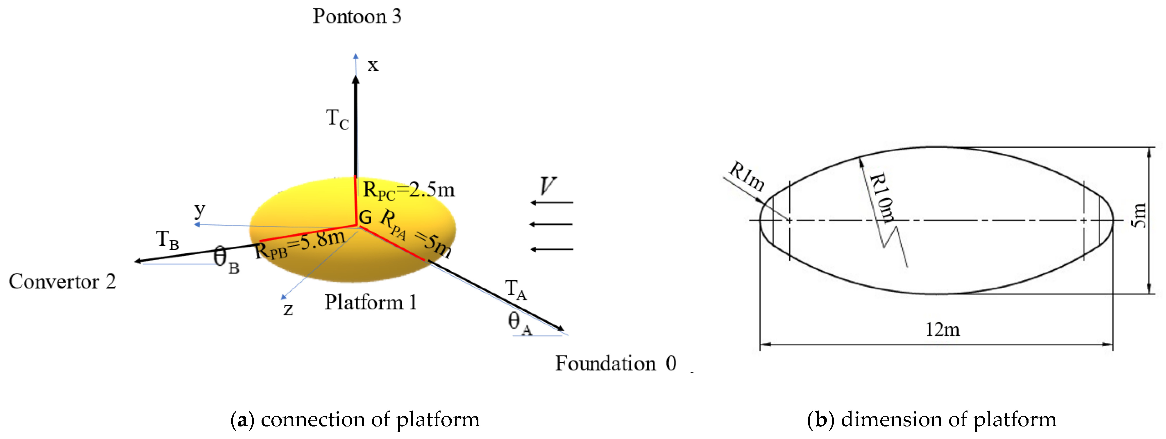
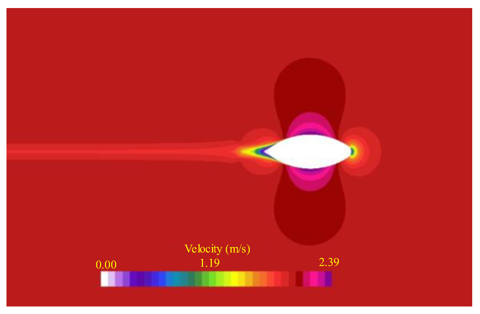
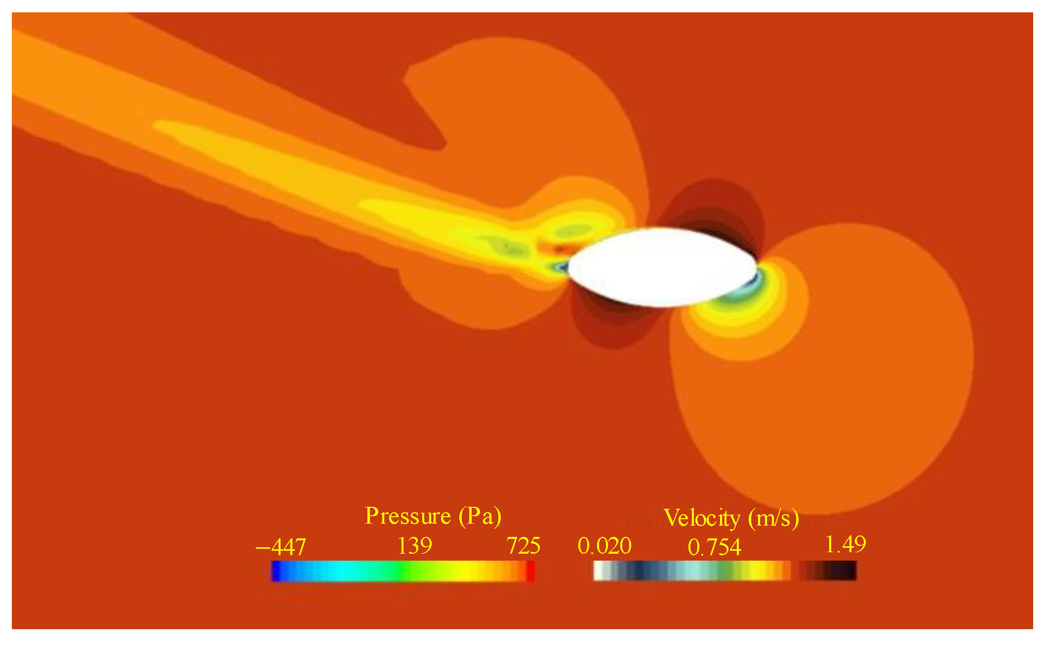
5.1. Hydrodynamic Parameter of Floating Platform

5.1.1. Dimension of Platform

To reduce hydrodynamic drag on the platform and to avoid disturbing the current through the turbine, the following oval configuration is designed as shown in Figure 3.

5.1.2. Hydrodynamic Damping and Stiffness Parameters of Platform

Because the hydrodynamic forces and moments on the floating platform due to the FSI are expressed in Taylor series, the hydrodynamic damping parameter of platform can be determined by the two methods: (1) determine these forces and moments by using the commercial STAR-CCM⁺ software, (2) calculate the hydrodynamic parameter based on the determined forces and moments.

Firstly, given $\left(V,{\dot{x}}_{1d},{\dot{y}}_{1d},{\dot{z}}_{1d},{\phi }_{1x},{\phi }_{1y},{\phi }_{1z},{\dot{\phi }}_{1x},{\dot{\phi }}_{1y},{\dot{\phi }}_{1z}\right)=\left(V,0,0,0,0,0,0,0,0,0\right),$ $0<V<2.5 \mathrm{m}/\mathrm{s}$ and by using the commercial STAR-CCM software, it is determined that the hydrodynamic forces and moments are $f_{Px}=f_{Pz}=m_{Px}=m_{Py}=m_{Pz}=0,$ because of the symmetry of the platform. The hydrodynamic drag is

$$f_{pys}=f_{Py}\left(V,0,0,0,0,0,0,0,0,0\right)=C_{py}\frac{1}{2}\rho A_{Py}{V}^2,$$

(81)

where the cross-sectional area of the platform $A_{Py}=19.635 {\mathrm{m}}^2$. According to the numerical hydrodynamic drag with different current velocity V, the drag coefficient $C_{py}=0.034$. The flow field around the platform is shown in Figure 4 with $V=1 \mathrm{m}/\mathrm{s}$. It is observed that the velocity around the platform is symmetrical. The current near the platform will be disturbed.

Secondly, considering the condition,$\left(V,{\dot{x}}_{1d},{\dot{y}}_{1d},{\dot{z}}_{1d},{\phi }_{1x},{\phi }_{1y},{\phi }_{1z},{\dot{\phi }}_{1x},{\dot{\phi }}_{1y},{\dot{\phi }}_{1z}\right)=$ $\left(V,{\dot{x}}_{1d},0,0,0,0,0,0,0,0\right),$ and given n sets of parameters $0<V<2.5 \mathrm{m}/\mathrm{s},-1.5<{\dot{x}}_{1d}<0$, these n sets of numerical hydrodynamic forces and moments are calculated by using the commercial STAR-CCM software. The flow field around the platform is shown in Figure 5 with $\left\{V=1 \mathrm{m}/\mathrm{s},{\dot{x}}_{1d}=-0.5 \mathrm{m}/\mathrm{s}\right\}$. It is observed that the velocity around the platform is asymmetrical. The hydrodynamic heaving force will be induced. Based on the formula

$$f_{Pj}\left(V,{\dot{x}}_{1d},0,0,0,0,0,0,0,0\right)=f_{Pj}\left(V,0,0,0,0,0,0,0,0,0\right)+\frac{\partial f_{Pj}}{\partial {\dot{x}}_{1d}}{\dot{x}}_{1d},j=x,y,z,$$

$$m_{Pj}\left(V,{\dot{x}}_{1d},0,0,0,0,0,0,0,0\right)=m_{Pj}\left(V,0,0,0,0,0,0,0,0,0\right)+\frac{\partial m_{Pj}}{\partial {\dot{x}}_{1d}}{\dot{x}}_{1d},j=x,y,z,$$

(82)

one can determine the hydrodynamic parameters $\left\{\partial m_{Pj}/\partial {\dot{x}}_{1d},\partial m_{Pj}/\partial {\dot{x}}_{1d}\right\},j=x,y,z$. In the similar way, other hydrodynamic parameters are obtained and listed in Appendix B.

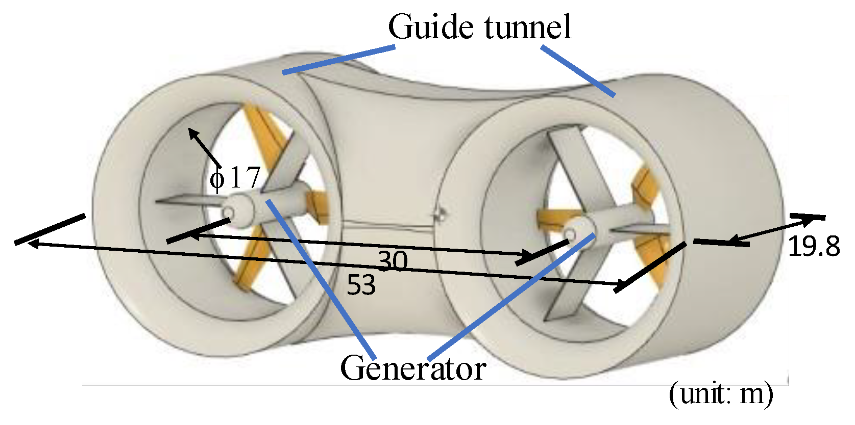
5.2. Hydrodynamic Parameter of Convertor

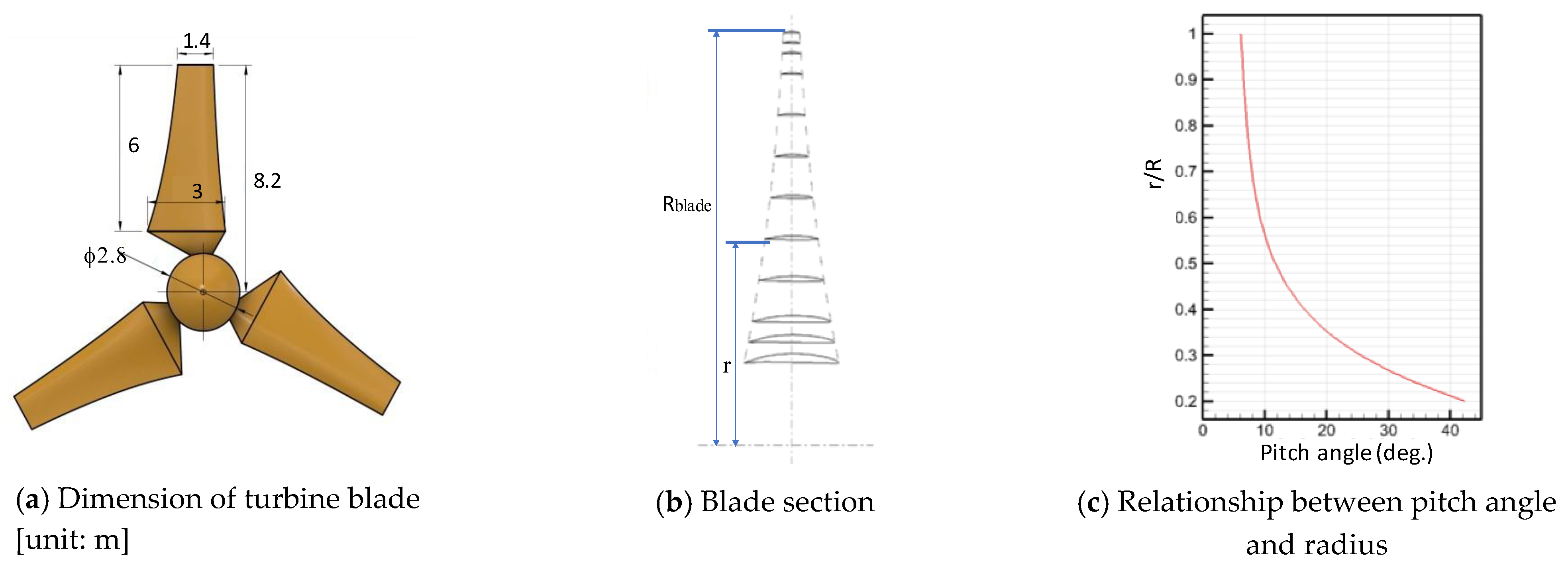
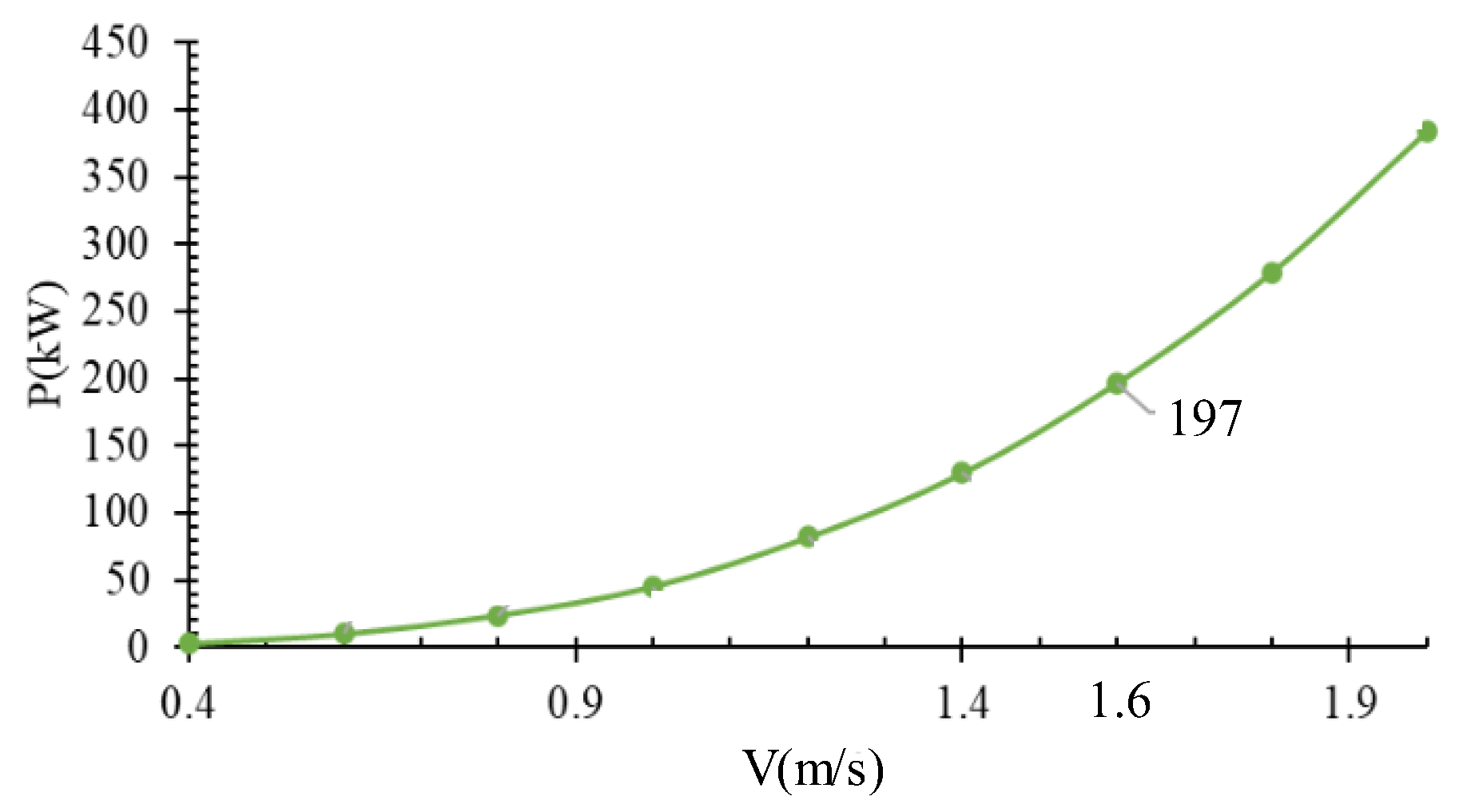
5.2.1. The Turbine Blade and Its Performance

The ocean energy convertor is composed of two turbine generators and an integration structure, as shown in Figure 6. Its normal power generation is 400 kW. The blade shape is shown in Figure 7.

The two turbine blades rotate reversely at the same rotating speed for rotational balance. Under the current velocity V = 2 m/s, the velocity field around the fixed convertor with rotating blade at the tip speed ratio TSR = 3.5 is calculated by using Star CCM+ and shown in Figure 8. It is observed that the current flows through the turbine blade along the guide tunnel. It will increase the flow velocity through the blade and the power generation. Moreover, the flow field around the two turbine blades will not disturbs each other. Figure 9 shows the effect of the TSR on the power coefficient of the turbine, CP = power/$\left(\frac{1}{2}\rho A{V}^3\right)$, at the current velocity V = 2 m/s. The maximum power coefficient CP of the proposed turbine is 0.43 at TSR = 3.5.

Further, Figure 10 shows the relation between the current velocity V and the output power at TSR = 3.5. It is determined that when the current velocity V = 1.6 m/s, the power of each turbine P_each = 197 kW and the total output power of the two turbines is 394 kW. It is close to the nominal power of 400 kW.

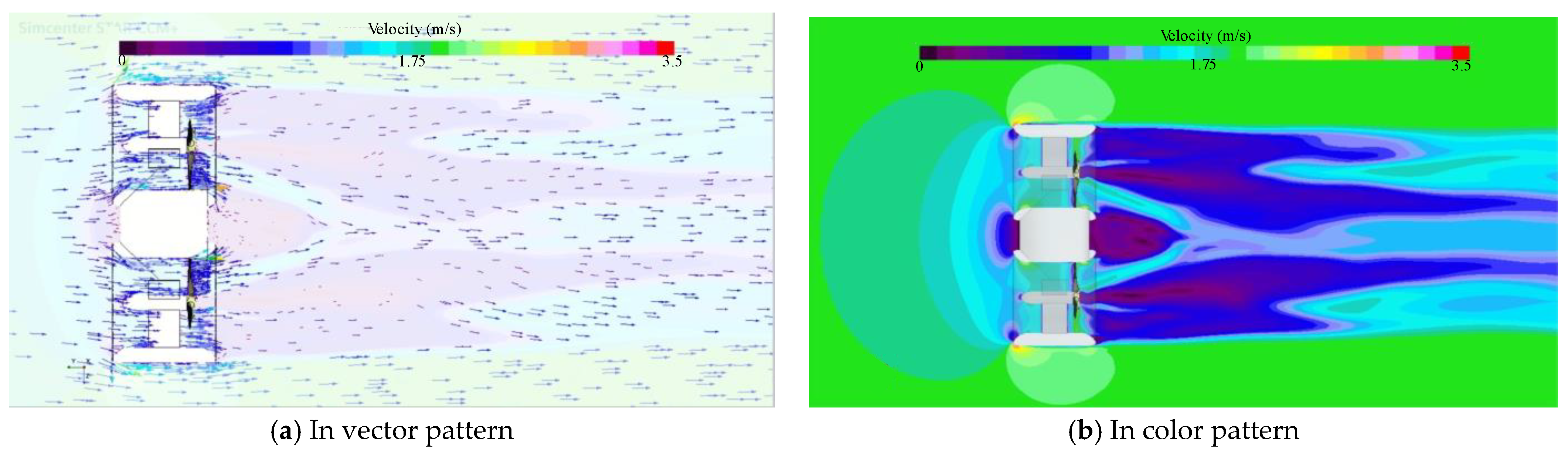
5.2.2. Hydrodynamic Damping Parameter of Convertor

Because the hydrodynamic force and moment due to the motion of the convertor are expressed in Taylor series, its hydrodynamic damping parameters can be determined as follows:

Firstly, given $\left(V,{\dot{x}}_{2d},{\dot{y}}_{2d},{\dot{z}}_{2d},{\phi }_{2x},{\phi }_{2y},{\phi }_{2z},{\dot{\phi }}_{2x},{\dot{\phi }}_{2y},{\dot{\phi }}_{2z},TSR\right)=\left(V,0,0,0,0,0,0,0,0,0,3.5\right),$ 0 < V< 2.5 m/s, and by using the commercial STAR-CCM⁺ software, the hydrodynamic forces and moments are $f_{Tx}=f_{Tz}=m_{Tx}=m_{Ty}=m_{Tz}=0,$ because of the symmetry of the convertor. The hydrodynamic drag is

$$f_{Tys}\left(V,0,0,0,0,0,0,0,0,0,3.5\right)=C_{Tfy}\frac{1}{2}\rho A_{Tfy}{V}^2,$$

(83)

where the cross-sectional area of the convertor $A_{Tfy}=1034 {\mathrm{m}}^2$. According to the numerical hydrodynamic drag with different current velocity V, the drag coefficient $C_{Tfy}=0.50$. The flow field around the convertor is shown in Figure 8 with $V=2 \mathrm{m}/\mathrm{s}$.

Secondly, considering the condition, $\left(V,{\dot{x}}_{2d},{\dot{y}}_{2d},{\dot{z}}_{2d},{\phi }_{2x},{\phi }_{2y},{\phi }_{2z},{\dot{\phi }}_{2x},{\dot{\phi }}_{2y},{\dot{\phi }}_{2z},TSR\right)$ = $(V,{\dot{x}}_{2d},0,0,0,$ $0,0,0,0,0,3.5),$ $0<V<2.5 \mathrm{m}/\mathrm{s},-1.5<{\dot{x}}_{2d}<0$, the numerical hydrodynamic forces and moments are calculated.

Finally, based on the formula

$$f_{Tj}\left(V,{\dot{x}}_{2d},0,0,0,0,0,0,0,0,3.5\right)=f_{Tj}\left(V,0,0,0,0,0,0,0,0,0,3.5\right)+\frac{\partial f_{Tj}}{\partial {\dot{x}}_{2d}}{\dot{x}}_{2d},$$

$$m_{Tj}\left(V,{\dot{x}}_{2d},0,0,0,0,0,0,0,0,3.5\right)=m_{Pj}\left(V,0,0,0,0,0,0,0,0,0,3.5\right)+\frac{\partial m_{Tj}}{\partial {\dot{x}}_{2d}}{\dot{x}}_{2d},j=x,y,z$$

(84)

one can determine the hydrodynamic parameters $\left\{\partial m_{Tj}/\partial {\dot{x}}_{2d},\partial m_{Tj}/\partial {\dot{x}}_{2d}\right\},j=x,y,z$.

Similarly, other hydrodynamic parameters are obtained and listed in Appendix C.

6. Solution Method

6.1. Dynamic Displacement

Multiplying Equation (78) by the inverse matrix of mass $M^{-1}$, one obtains

$${\ddot{x}}_d+M^{-1}C{\dot{x}}_d+M^{-1}K{x}_d=M^{-1}{F}_d=F_{dc}\cos \Omega t+F_{ds}\sin \Omega t.$$

(85)

Assume the solution of Equation (85),

$$z_d=z_{dc}\cos \Omega t+z_{ds}\sin \Omega t,$$

(86)

where

$$\begin{array}{l}{z}_{dc}={\left[\begin{array}{cccccccccccccccccc}{x}_{1dc}& y_{1dc}& z_{1dc}& x_{2dc}& y_{2dc}& z_{2dc}& x_{3dc}& y_{3dc}& z_{3dc}& x_{4dc}& y_{4dc}& z_{4dc}& {\phi }_{Txc}& {\phi }_{Tyc}& {\phi }_{Tzc}& {\phi }_{Pxc}& {\phi }_{Pyc}& {\phi }_{Pzc}\end{array}\right]}^T\\ z_{ds}={\left[\begin{array}{cccccccccccccccccc}{x}_{1ds}& y_{1ds}& z_{1ds}& x_{2ds}& y_{2ds}& z_{2ds}& x_{3ds}& y_{3ds}& z_{3ds}& x_{4ds}& y_{4ds}& z_{4ds}& {\phi }_{Txs}& {\phi }_{Tys}& {\phi }_{Tzs}& {\phi }_{Pxs}& {\phi }_{Pys}& {\phi }_{Pzs}\end{array}\right]}^T\end{array}.$$

Substituting the solution (86) into Equation (85), one obtains

$$\begin{array}{l}-{\Omega }^{2}I\left(z_{dc}\cos \Omega t+z_{ds}\sin \Omega t\right)+M^{-1}C\left(-\Omega z_{dc}\sin \Omega t+\Omega z_{ds}\cos \Omega t\right)\\ +M^{-1}K\left(z_{dc}\cos \Omega t+z_{ds}\sin \Omega t\right)=F_{ds}\sin \Omega t+F_{dc}\cos \Omega t\end{array}.$$

(87)

By using the balanced method for Equation (87), one obtains

$$z_{dc}=-\Omega A^{-1}\left(M^{-1}C\right)z_{ds}+A^{-1}{F}_{dc}$$

(88)

and

$$A{z}_{ds}-\Omega M^{-1}C{z}_{dc}=F_{ds},$$

(89)

where $A=\left(M^{-1}K-{\Omega }^{2}I\right)$. Substituting Equation (88) into (89), one obtains

$$z_{ds}={\left(A+{\Omega }^2\left(M^{-1}C\right)A^{-1}\left(M^{-1}C\right)\right)}^{-1}\left\{F_{ds}+\Omega \left(M^{-1}C\right)A^{-1}{F}_{dc}\right\}.$$

(90)

Based on Equation (90), the frequency equation is obtained:

$$\left|A+{\Omega }^2\left(M^{-1}C\right)A^{-1}\left(M^{-1}C\right)\right|=0.$$

(91)

6.2. Dynamic Tensions of Ropes

Under regular wave, the dynamic tensions of Ropes A, B, C, D are

$$T_{Ad}=T_{Adc}\cos \Omega t+T_{Ads}\sin \Omega t, \left|T_{Ad}\right|=\sqrt{T_{Adc}^2+T_{Ads}^2},$$

(92)

$$\mathrm{where} T_{Adc}=K_{Ad}\left(\frac{x_{1s}}{L_A}{x}_{1dc}+\frac{y_{1s}}{L_A}{y}_{1dc}\right), T_{Ads}=K_{Ad}\left(\frac{x_{1s}}{L_A}{x}_{1ds}+\frac{y_{1s}}{L_A}{y}_{1ds}\right).$$

$$T_{Bd}=T_{Bdc}\cos \Omega t+T_{Bds}\sin \Omega t, \left|T_{Bd}\right|=\sqrt{T_{Bdc}^2+T_{Bds}^2},$$

(93)

$$\begin{array}{l}\mathrm{where} T_{Bdc}=K_{Bd}\left[\frac{x_{2s}-x_{1s}}{L_B}\left(x_{2dc}-x_{1dc}\right)+\frac{y_{2s}-y_{1s}}{L_B}\left(y_{2dc}-y_{1dc}\right)\right],\\ T_{Bds}=K_{Bd}\left[\frac{x_{2s}-x_{1s}}{L_B}\left(x_{2ds}-x_{1ds}\right)+\frac{y_{2s}-y_{1s}}{L_B}\left(y_{2ds}-y_{1ds}\right)\right].\end{array}.$$

$$T_{Cd}=T_{Cdc}\cos \Omega t+T_{Cds}\sin \Omega t, \left|T_{Cd}\right|=\sqrt{T_{Cdc}^2+T_{Cds}^2},$$

(94)

$$\mathrm{where} T_{Cdc}=K_{Cd}\left(x_{3dc}-x_{1dc}\right), T_{Cds}=K_{Cd}\left(x_{3ds}-x_{1ds}\right).$$

$$T_{Dd}=T_{Ddc}\cos \Omega t+T_{Dds}\sin \Omega t, \left|T_{Dd}\right|=\sqrt{T_{Ddc}^2+T_{Dds}^2},$$

(95)

$$\mathrm{where} T_{Ddc}=K_{Dd}\left(x_{4dc}-x_{2dc}\right), T_{Dds}=K_{Dd}\left(x_{4ds}-x_{2ds}\right).$$

7. Numerical Results and Discussion

Consider the conditions: (1) H_bed = 1300 m, (2) A_BX = 4 m², (3) A_BT = 4 m², (4) HSPE rope: E_PE = 100 GPa, w_PE = 16.22 kg/m, D_PE = 154 mm, A_PE = 0.0186 m², T_fracture = 759 tons, (5) L_C = L_D = 60 m, (6) L_E = 150 m, (7) ${\theta }_A=30°$, (8) V = 1.6 m/s, (9) H_wave = 16 m and λ = 156 m. (10) $M_1=300 \mathrm{tons}$, $M_2=538 \mathrm{tons}$, $M_3=M_4=250 \mathrm{tons}$, (11) $I_{Tx}=8.940\times {10}^{10} \mathrm{kg}-{\mathrm{m}}^2$, $I_{Ty}=2.712\times {10}^{10} \mathrm{kg}-{\mathrm{m}}^2$, $I_{Tz}=8.940\times {10}^{10} \mathrm{kg}-{\mathrm{m}}^2$;$I_{Px}=3.0\times {10}^8 \mathrm{kg}-{\mathrm{m}}^2$, $I_{Py}=5.0\times {10}^6 \mathrm{kg}-{\mathrm{m}}^2$, $I_{Pz}=3.0\times {10}^8 \mathrm{kg}-{\mathrm{m}}^2$, (12) the hydrodynamic damping and stiffness parameters ${\left(\partial f_{ki}/\partial s_{kj}\right)}_0\mathrm{and} {\left(\partial m_{ki}/\partial s_{kj}\right)}_0$ are listed in Section 5, (13) the performance of convertor is presented in Section 5, (14) T_AS = 78.07 tons, T_Bs = 67.53 tons, T_Cs = 80 tons, and T_Ds = 80 tons, (15) α = 30°.

Figure 11a demonstrates the spectrum of dynamic tension of rope. It is determined that the resonant frequency is 0.110 Hz. The resonant dynamic tension of ropes: T_Ad = 84.56 tons. T_Bd = 68.04 tons T_Cd = 32.18 tons, and T_Dd = 32.13 tons. These are greatly smaller than the fracture strength of rope T_fracture = 759 tons. Figure 11b demonstrates the translational displacements of the platform, the convertor, the pontoons 3 and 4. It is observed that the resonant surge displacements of the pontoons y_3d and y_4d are very significant. The sway displacements z_1d and z_2d are very small. The maximum heave, surge and sway displacements x_2d, y_2d, and z_2d of the convertor are 3.21, 4.29 and 0.292 m, respectively. It is observed from Figure 11c that the maximum yawing, rolling and pitching angles of the platform ${\phi }_{Px}$, ${\phi }_{Py}$, and ${\phi }_{Pz}$ are 0.26°, 5.83° and 54.4°, respectively. The maximum yawing, rolling and pitching angles of the convertor ${\phi }_{Tx}$, ${\phi }_{Ty}$, and ${\phi }_{Tz}$ are 0.005°, 0.322° and 0.283°, respectively.

According to Figure 11b,c, the displacement of the platform is obviously larger than that of the convertor. Because the translational and rotational displacements of the convertor are small under the wave impact, the efficiency of power generation of convertor can be maintained to be high.

Obviously, the hydrodynamic damping parameters of the convertor and platform significantly depend on their configuration design. The dynamic performance of the system is decided by the corresponding hydrodynamic damping parameters or the configuration design. For clarity, the relationship between the hydrodynamic damping and the rope tension is investigated here. The hydrodynamic damping and stiffness parameters of some convertor and platform different to the proposed ones are assumed to be

$$\frac{\partial f_{ki}}{\partial s_{kj}}={\beta }_k{\left(\frac{\partial f_{ki}}{\partial s_{kj}}\right)}_0, \mathrm{and} \frac{\partial m_{ki}}{\partial s_{kj}}={\beta }_k{\left(\frac{\partial m_{ki}}{\partial s_{kj}}\right)}_0,$$

(96)

where the parameters with subscript ‘0′ are those presented in Section 5 and Figure 11. ${\beta }_k, k=P,T$ are the hydrodynamic parameter ratio of different convertors and platforms to those presented in Section 5.

In Figure 12, the hydrodynamic parameter ratios are assumed to be ${\beta }_P={\beta }_T=0.1$. Other parameters are the same as those in Figure 11. The effects of the small hydrodynamic parameters and the typhon wave frequency on the dynamic tensions of the ropes, T_Ad, T_Bd, T_Cd, and T_Dd, are studied. It is determined that the resonant frequencies are 0.032 and 0.160 Hz. The maximum resonant dynamic tension of ropes A, B, C, and D: T_Ad = 294.4 tons, T_Bd = 165.0 tons, T_Cd = 113.9 tons, and T_Dd = 48.9 tons. These are significantly larger than those in Figure 11a. Further, if the hydrodynamic damping and stiffness parameters of the convertor are neglected, i.e., ${\beta }_P=0.1$ and ${\beta }_T=0$. The dynamic tension spectrum is presented in Figure 13. It is observed from Figure 13 that without the hydrodynamic damping of the convertor, the resonant tensions are significantly increased. The resonant dynamic tensions are greatly larger than the fracture strength of rope T_fracture = 759 tons.

Figure 14a demonstrates the dynamic tension spectrum with L_C = 140 m and L_D = 60 m. In Figure 11a, with the rope lengths L_C = L_D = 60 m, the maximum dynamic tension T_Ad = 84.56 tons. In Figure 14a, with the rope lengths L_C = 140 m, L_D = 60 m, the maximum dynamic tension T_Cd = 171.8 tons. It is because the surge and heave displacements of the pontoon 3 and platform at the resonance in Figure 14b are significantly larger than those in Figure 11b. Moreover, the pitch angle of the platform in Figure 14c is significantly larger than that in Figure 11c.

Figure 15a demonstrates the dynamic tension spectrum with L_C = 60 m and L_D = 140 m. In Figure 11a, with L_C = L_D = 60 m, the maximum dynamic tension was T_Ad = 84.56 tons. In Figure 15a, the maximum dynamic tension T_Ad = 64.06 tons and T_Cd = 60.06 tons. It is observed from Figure 15b that the maximum resonance displacement is the surge of the pontoon 4. However, it is observed from Figure 11b that the maximum resonance displacement is the surge of the pontoon 3. In Figure 15c, the maximum yaw, roll and pitch angles of the platform ${\phi }_{1x}$, ${\phi }_{1\mathrm{y}}$, and ${\phi }_{1\mathrm{z}}$ are 1.3°, 2.5° and 21°, respectively. The maximum yaw, roll and pitch angles of the convertor ${\phi }_{2x}$, ${\phi }_{2\mathrm{y}}$, and ${\phi }_{2\mathrm{z}}$ are 0.01°, 0.104° and 0.027°, respectively. The maximum pitch angle of the platform in Figure 15c is significantly smaller than that in Figure 11c.

Figure 16 demonstrates the effect of the length L_C on the maximum dynamic tensions of ropes under 0.01 Hz < wave frequency f < 0.91 Hz and L_D = 60 m. It is observed that if 50 m < L_C < 130 m, all the dynamic tensions are under 130 tons. The maximum tension of rope C changes with the length L_C. It is because if the length L_C approaches 150 m, rope A and rope B are nearly in line and it results in the instability of the platform and the pontoon 3.

Figure 17 demonstrates the relation between the length L_D and the maximum dynamic tensions of ropes under 0.01 Hz < wave frequency f < 0.91 Hz and L_C = 60 m. It is determined that all dynamic tensions are under 90 tons. For 90 m < L_D < 130 m, all dynamic tensions are under 50 tons.

Figure 18 demonstrates the relation among the rope angle θ_A, the wave frequency f and the total tensions of ropes. It is observed that the angle θ_A will increase the resonant frequency; this is because if the angle θ_A is increased, the stiffness of system is increased. Moreover, if the angle θ_A is over critical, the dynamic tension T_A increases with the angle θ_A.

8. Conclusions

This paper presents the mathematical model of the coupled translational–rotational motions of the mooring system for an ocean energy convertor operating under the typhoon wave impact. The configurations of the convertor and the floating platform are designed. The hydrodynamic damping and stiffness parameters under the fluid–structure interaction are calculated. The performance of the mooring system under typhon wave impact and with different parameters is investigated and discovered as follows:

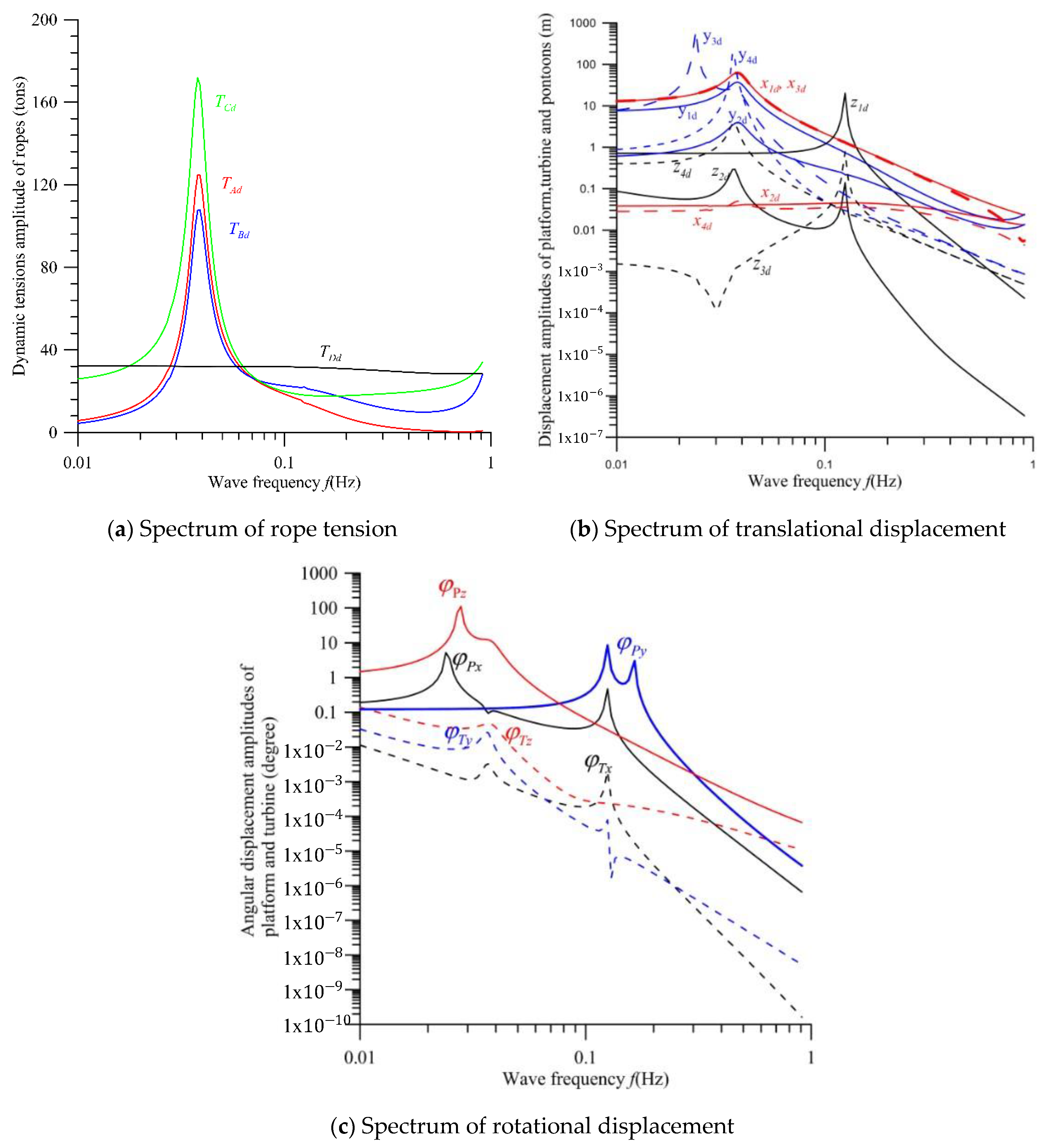
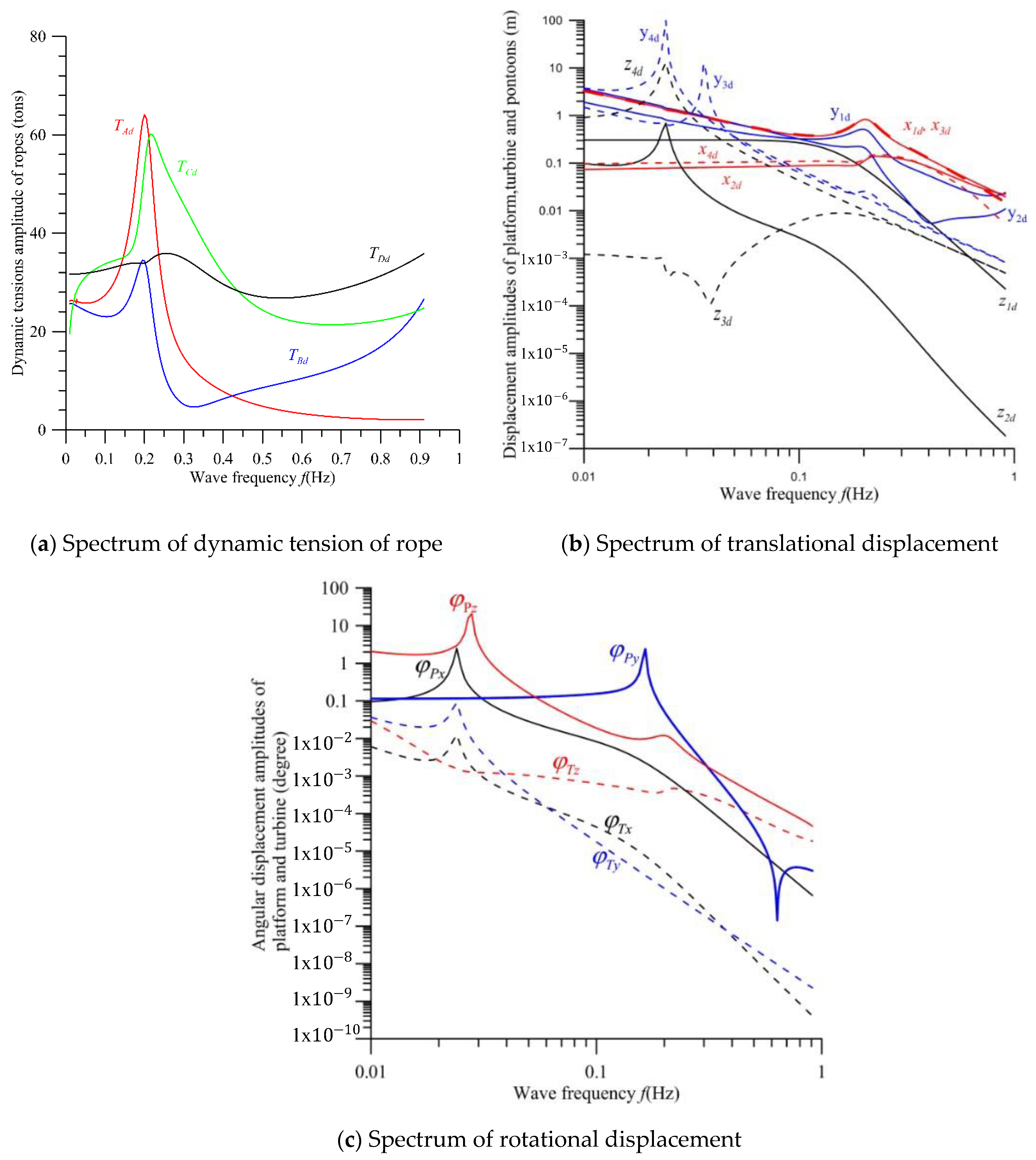
(1)

The translational displacements of pontoons 3 and 4 are more obvious than those of the platform and convertor.

(2)

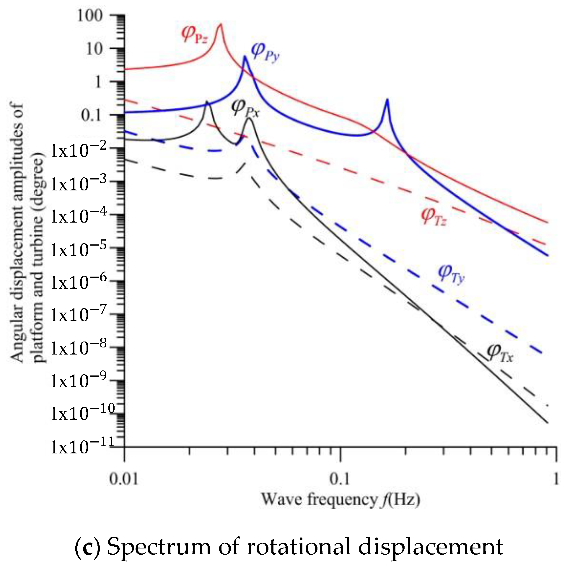
The angular displacement in pitch motion of the platform is greatly larger than those of the yaw and roll motions.

(3)

The translational and angular displacements of the platform are obviously higher than those of the convertor.

(4)

For this proposed mooring system, all the displacements of the convertor are kept small under the significant wave impact. Therefore, the relative flow velocity and direction of the convertor to the current are almost constant such that the power efficiency of convertor can maintain to be stable and high.

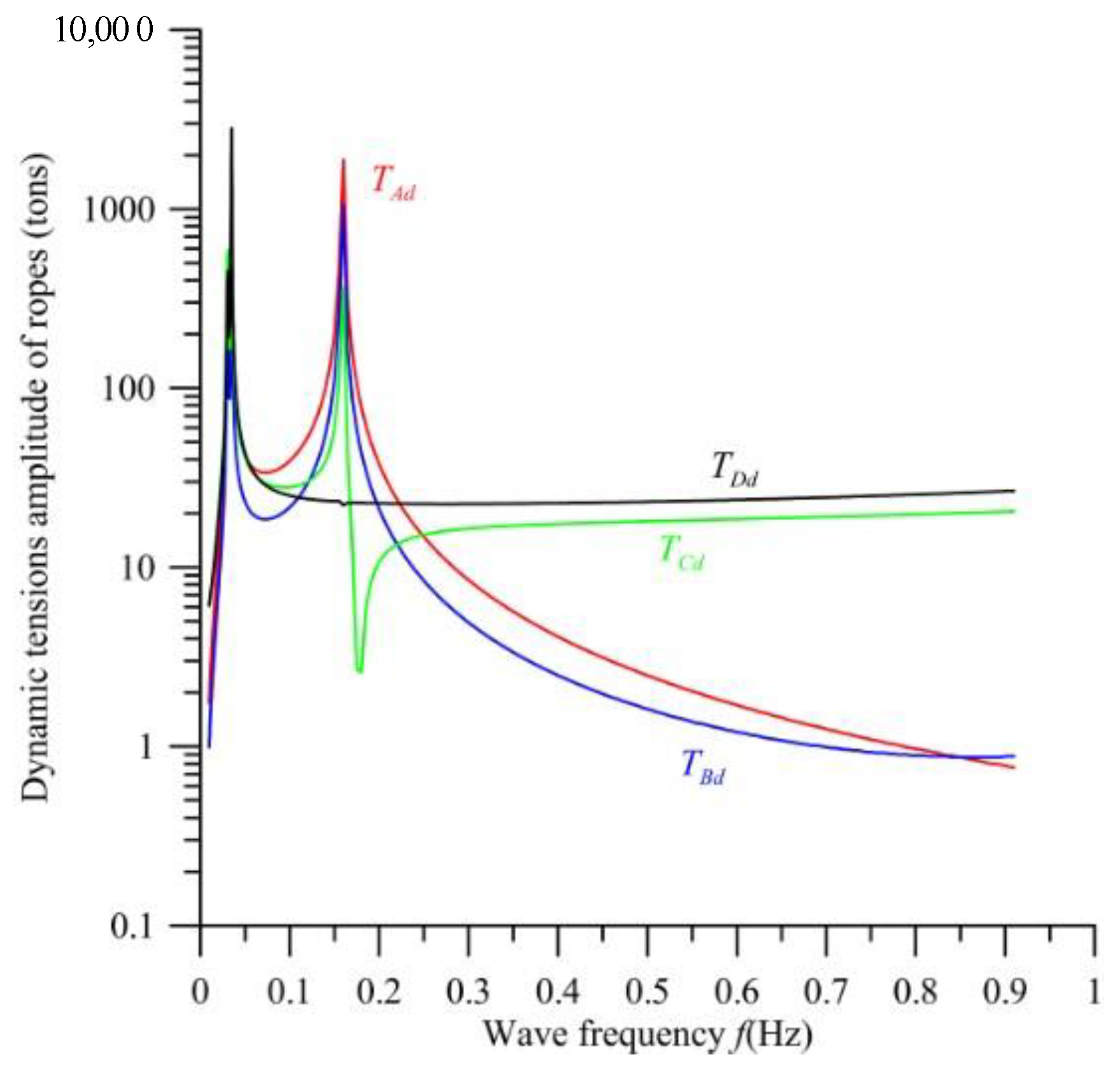
(5)

If there is a mooring system without the hydrodynamic damping of the convertor, the resonant tensions are significantly increased and greatly over than the rope fracture strength.

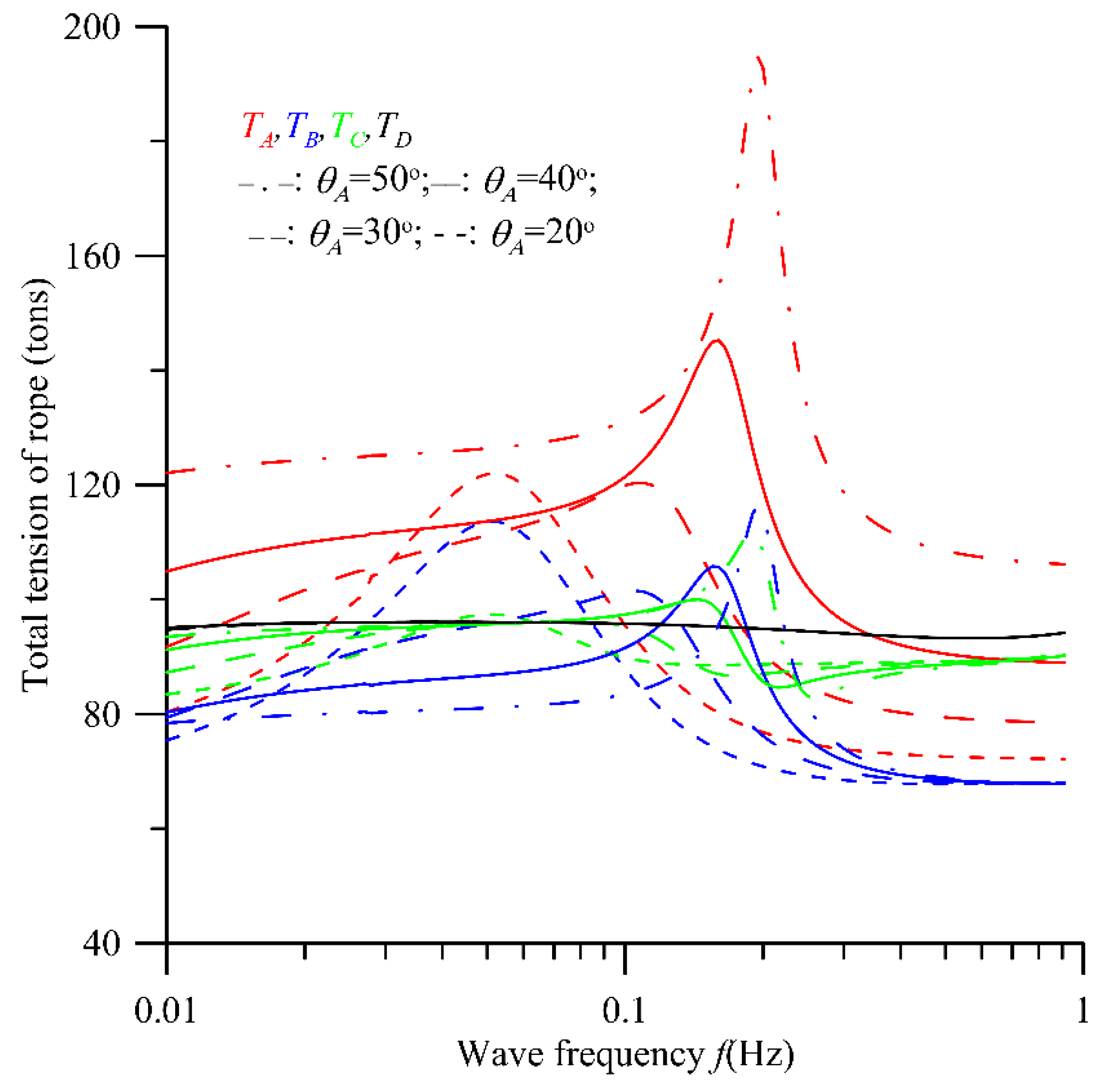
(6)

The resonant frequency of the mooring system and the total tension T_A increases with the setting angle θ_A of rope A.

References

- Chen, Y.Y.; Hsu, H.C.; Bai, C.Y.; Yang, Y.; Lee, C.W.; Cheng, H.K.; Shyue, S.W.; Li, M.S. Evaluation of test platform in the open sea and mounting test of KW Kuroshio power-generating pilot facilities. In Proceedings of the 2016 Taiwan Wind Energy Conference, Keelung, Taiwan, 24–25 November 2016. [Google Scholar]
- IHI; NEDO. The Demonstration Experiment of the IHI Ocean Current Turbine Located off the Coast of Kuchinoshima Island, Kagoshima Prefecture, Japan, 14 August 2017. Available online: https://tethys.pnnl.gov/project-sites/ihi-ocean-current-turbine (accessed on 28 August 2021).
- Nobel, D.R.; O’Shea, M.; Judge, F.; Robles, E.; Martinez, R.F.; Thies, P.R.; Johanning, L.; Corlay, R.; Davey, T.A.D.; Vejayan, N.; et al. Standardising Marine Renewable Energy Testing: Gap Analysis and Recommendations for Development of Standards. J. Mar. Sci. Eng. 2021, 9, 971. [Google Scholar] [CrossRef]
- Lin, S.M.; Chen, Y.Y.; Hsu, H.C.; Li, M.S. Dynamic Stability of an Ocean Current Turbine System. J. Mar. Sci. Eng. 2020, 8, 687. [Google Scholar] [CrossRef]
- C´atipovic, I.; Alujevic, N.; Rudan, S.; Slapničar, V. Numerical Modelling for Synthetic Fibre Mooring Lines Taking Elongation and Contraction into Account. J. Mar. Sci. Eng. 2021, 9, 417. [Google Scholar] [CrossRef]
- Lin, S.M.; Chen, Y.Y. Dynamic stability and protection design of a submarined floater platform avoiding Typhoon wave impact. J. Mar. Sci. Eng. 2021, 9, 977. [Google Scholar] [CrossRef]
- Lin, S.M.; Chen, Y.Y.; Liauh, C.T. Dynamic stability of the coupled pontoon-ocean turbine-floater platform-rope system under harmonic wave excitation and steady ocean current. J. Mar. Sci. Eng. 2021, 9, 1425. [Google Scholar] [CrossRef]
- Lin, S.M.; Liauh, C.T.; Utama, D.W. Design and dynamic stability analysis of a submersible ocean current generator-platform mooring system under typhoon irregular wave. J. Mar. Sci. Eng. 2022, 10, 538. [Google Scholar] [CrossRef]
- Davidson, J.; Ringwood, J.V. Mathematical Modelling of Mooring Systems for Wave Energy Converters—A Review. Energies 2017, 10, 666. [Google Scholar] [CrossRef] [Green Version]
- Chen, D.; Nagata, S.; Imai, Y. Modelling wave-induced motions of a floating WEC with mooring lines using the SPH method. In Proceedings of the 3rd Asian Wave and Tidal Energy Conference, Marina Bay Sands, Singapore, 25–27 October 2016; pp. 24–28. [Google Scholar]
- Xiang, G.; Xu, S.; Wang, S.; Soares, C.G. Advances in Renewable Energies Offshore: Comparative Study on Two Different Mooring Systems for a Buoy; Taylor & Francis Group: London, UK, 2019; pp. 829–835. [Google Scholar]
- Paduano, B.; Giorgi, G.; Gomes, R.P.F.; Pasta, E.; Henriques, J.C.C.; Gato, L.M.C.; Mattiazzo, G. Experimental Validation and Comparison of Numerical Models for the Mooring System of a Floating Wave Energy Converter. J. Mar. Sci. Eng. 2020, 8, 565. [Google Scholar] [CrossRef]
- Touzon, I.; Nava, V.; Miguel, B.D.; Petuya, V. A Comparison of Numerical Approaches for the Design of Mooring Systems for Wave Energy Converters. J. Mar. Sci. Eng. 2020, 8, 523. [Google Scholar] [CrossRef]
- Xiang, G.; Xiang, X.; Yu, X. Dynamic Response of a SPAR-Type Floating Wind Turbine Foundation with Taut Mooring System. J. Mar. Sci. Eng. 2022, 10, 1907. [Google Scholar] [CrossRef]
- Anagnostopoulos, S.A. Dynamic response of offshore platforms to extreme waves including fluid-structure interaction. Eng. Struct. 1982, 4, 179–185. [Google Scholar] [CrossRef]
- Bose, C.; Badrinath, S.; Gupta, S.; Sarkar, S. Dynamical stability analysis of a fluid structure interaction system using a high fidelity Navier-Stokes solver. Procedia Eng. 2016, 144, 883–890. [Google Scholar] [CrossRef] [Green Version]
- Belibassakis, K.A. A boundary element method for the hydrodynamic analysis of floating bodies in variable bathymetry regions. Eng. Anal. Bound. Elem. 2008, 32, 796–810. [Google Scholar] [CrossRef]
- Tsui, Y.Y.; Huang, Y.C.; Huang, C.L.; Lin, S.W. A finite-volume-based approach for dynamic fluid-structure interaction. Numer. Heat Transf. Part B Fundam. 2013, 64, 326–349. [Google Scholar] [CrossRef]
- Xiang, T.; Istrati, D.; Yim, S.C.; Buckle, I.G. Tsunami Loads on a Representative Coastal Bridge Deck: Experimental Study and Validation of Design Equations. J. Waterw. Port Coast. Ocean. Eng. 2020, 146, 04020022. [Google Scholar] [CrossRef]
- Westphalen, J.; Greaves, D.M.; Raby, A.; Hu, Z.Z.; Causon, D.M.; Mingham, C.G.; Omidvar, P.; Stansby, P.K.; Rogers, B.D. Investigation of wave-structure interaction using state of the art CFD techniques. Open J. Fluid Dyn. 2014, 4, 18. Available online: https://www.scirp.org/journal/paperinformation.aspx?paperid=43397 (accessed on 20 December 2022). [CrossRef] [Green Version]
- Hasanpour, A.; Istrati, D.; Buckle, I. Coupled SPH–FEM Modeling of Tsunami-Borne Large Debris Flow and Impact on Coastal Structures. J. Mar. Sci. Eng. 2021, 9, 1068. [Google Scholar] [CrossRef]
- Lin, S.M. Energy dissipation and dynamic response of an AM-AFM subjected to a tip-sample viscous force. Ultramicroscopy 2007, 107, 245–253. [Google Scholar] [CrossRef] [PubMed]
Disclaimer/Publisher’s Note: The statements, opinions and data contained in all publications are solely those of the individual author(s) and contributor(s) and not of MDPI and/or the editor(s). MDPI and/or the editor(s) disclaim responsibility for any injury to people or property resulting from any ideas, methods, instructions or products referred to in the content. |
© 2023 by the authors. Licensee MDPI, Basel, Switzerland. This article is an open access article distributed under the terms and conditions of the Creative Commons Attribution (CC BY) license (https://creativecommons.org/licenses/by/4.0/).
Share and Cite
Lin, S.-M.; Utama, D.W.; Liauh, C.-T. Coupled Translational–Rotational Stability Analysis of a Submersible Ocean Current Converter Platform Mooring System under Typhoon Wave. J. Mar. Sci. Eng. 2023, 11, 518. https://doi.org/10.3390/jmse11030518
Lin S-M, Utama DW, Liauh C-T. Coupled Translational–Rotational Stability Analysis of a Submersible Ocean Current Converter Platform Mooring System under Typhoon Wave. Journal of Marine Science and Engineering. 2023; 11(3):518. https://doi.org/10.3390/jmse11030518
Chicago/Turabian StyleLin, Shueei-Muh, Didi Widya Utama, and Chihng-Tsung Liauh. 2023. "Coupled Translational–Rotational Stability Analysis of a Submersible Ocean Current Converter Platform Mooring System under Typhoon Wave" Journal of Marine Science and Engineering 11, no. 3: 518. https://doi.org/10.3390/jmse11030518