Variations of Bottom Boundary Layer Turbulence under the Influences of Tidal Currents, Waves, and Raft Aquaculture Structure in a Shallow Bay

Abstract

High-frequency measurements of tides, waves, and turbulence were made using the bottom-mounted tripod equipped with the Nortek 6-MHz acoustic Doppler velocimetry during 20–23 February 2016 (winter) and 12–26 June 2017 (summer) in Heini Bay, Yellow Sea. The synchro-squeezed wavelet transform was applied for wave-turbulence decomposition, and an iterative procedure was developed to identify the turbulence inertial subrange in the bottom boundary layer. The analysis results reveal the dependency of the inertial subrange on the tidal current and turbulence intensities. The flood-ebb tidal flows are different between the summer and winter seasons, without and with the presence of dense raft aquaculture for kelp, respectively. In summer, the turbulent kinetic energy (TKE), turbulent Reynolds stress (TRS), and dissipation rate ($\epsilon$) of TKE increase smoothly with the increasing tidal flow magnitude, and $\epsilon$ is approximately in balance with TKE production related to the vertical shear. The presence of heavy kelp aquaculture in winter causes the reduction in flow speeds and TRS, while keeping TKE and $\epsilon$ at high levels.

1. Introduction

In shallow seas, the energetic turbulent motions in the bottom boundary layer (BBL) impact the resuspension and settling of sediments [1,2,3,4,5] and also the fluxes of dissolved matter on the seabed [6,7]. The BBL turbulence can also extend to the water column, thus affecting stratification and circulation [8,9]. Hence, quantifying the variations of BBL turbulence is important for improving the understanding and prediction of mass transports in shallow seas.

Over the past two decades, ocean turbulence has been more feasibly measured with the advent of new instruments such as the vertical micro-structure profiler (VMP), particle image velocimetry (PIV), the acoustic Doppler current profiler (ADCP), and acoustic Doppler velocimetry (ADV). VMP measures the micro-scale velocity shear that enables the estimation of the profiles of the dissipation rate ($\epsilon$) of turbulent kinetic energy (TKE) [10,11,12,13]. PIV measures the spatial distribution of velocity at high sample rates that can enable the direct estimation of the production and dissipation rates of TKE [14]. Broadband ADCP measures velocities along its multi-beams, enabling the estimation of the profiles of turbulent Reynolds stress (TRS) using the “variance method” and the velocity shear. The multiplying of TRS and shear gives the production rate of TKE [15,16,17,18]. Using the “spectral and structure function methods”, the ADCP measurements can also provide estimates of profiles of $\epsilon$ [19,20,21,22]. It is worth noting that the noise level and sampling frequency/space of the ADCP measurements may limit the estimation of turbulent quantities [15,23]. ADV takes point measurement of velocities with high sampling rates and low noise level, enabling the estimation of $\epsilon$ through fitting the velocity spectra in the inertial subrange and TRS through directly calculating the covariance of velocity fluctuations. The time series of $\epsilon$ and TRS from ADV measurements have been widely obtained for BBL turbulence studies [24,25,26,27,28].

In shallow seas where tidal flow is the dominated motion, the BBL turbulent parameters vary with the tidal flow. For example, measurements have revealed stronger BBL tidal flow corresponding to larger $\epsilon$ [6,7,26]. When impacts of surface waves are significant in the BBL, wave–current interactions occur [29,30,31,32,33]. Zhang et al. [34] simulated the generation of energetic turbulence due to enhanced shear in the BBL with the presence of wave–current interaction. Based on observational data, MacVean and Lacy [35] discovered that waves contributed to TKE production in the BBL.

Turbulence in the BBL is also impacted by water column stratification in shallow seas. Previous observational studies have revealed the constraint on the turbulence mixing length by stratification in the Hudson River estuary [36] and the York River estuary [37]. On the New England Shelf, in summer, the upward extension of the BBL turbulence is prohibited by the lower layer (above BBL) stratification generated by the combination of subtidal Ekman onshore bottom transport and the cross-shore density gradient [38].

In nearshore waters, the presence of high-density aquaculture structures can also have significant impacts on hydrodynamics [39,40,41,42]. In the microtidal Danish Limfjorden, Stevens and Petersen [43] observed the influences of turbulent flow and mixing through the suspended canopy formed by a shellfish aquaculture farm. The influence was two-way in that the turbulence was partially driven by the canopy and, in turn, the canopy reduced the flow speeds and turbulence within its interior. Near the Nanji Islands in the East China Sea, Xu et al. [44] observed the persistence of enhanced turbulent mixing due to the interaction of tidal flow and aquaculture structure.

Based on the above review of the previous studies, it is evident that the BBL turbulence in shallow seas is impacted by variations of flow, waves, and stratification due to water temperature and salinity, as well as the presence of aquaculture structure. It remains challenging to quantify the contributions from these various factors on the BBL turbulence. All these factors are present in Heini Bay (HB) in the Yellow Sea (Figure 1). In this study, we analyze long-term mooring observations in this region with the goal to derive new analysis methods and quantifications. Section 2 describes the study area and field observations. Section 3 presents the observed hydrodynamic conditions. Section 4 introduces the estimation of turbulence parameters. Section 5 analyzes the variations of turbulence and the inertial subrange. Section 6 provides the summary of the conclusions.

2. Study Area and Observations

The study area is HB located along the western coast of the Yellow Sea (Figure 1). HB has quite an open mouth. To the west of the straight line connecting the headlands along the northern and southern sides, the water depth is less than 10 m. The bed sediments consist mainly of silty sand in the intertidal flat and muddy silt in the remaining regions [45]. HB is under a slightly erosional condition [46]. There are no rivers flowing into the bay, and the water mass is mainly composed of the coastal water of the Yellow Sea. HB is often influenced by waves and monsoons.

HB has extensive areas for kelp aquaculture, extending from the shore to beyond the 20 m isobaths (approximately the region outlined by the green curve in Figure 1). The kelp seedlings are suspended along the long ropes attached to the sea surface rafts, enabling the kelp to grow through absorbing nutrients in seawater. The presence of a significant amount of kelp in water impacts the flows of seawater. In the Sungo Bay to the north of HB, Shi and Wei [47] found that the presence of raft aquaculture reduced the flow speed by 40% and prolonged the “half-life time” for water exchange by 71%, compared with the conditions in the absence of aquaculture.

Two mooring stations, HB1 and SH3, were located in the northern part of HB (Figure 1). At each station, a Campbell Scientific Datalogger CR1000 auto-meteorological station (AMS) was mounted on the sea surface buoy, and a tripod deployed on the seabed was equipped with a Nortek 6-MHz ADV.

Table 1. Summary of mooring observations.

Station	Latitude/Longitude (°N/°E)	Measurement Time	Mean Water Depth (m)	Instrument	Position of Observation (mab 2)	Sediment Type 3
HB1	37.03/122.56	20 January 2016–23 February 2016	7.5	ADV 1	0.45	Muddy silt
SH3	37.03/122.57	12 June 2017–26 June 2017	8.8	ADV	0.35	Muddy silt

¹ Acoustic Doppler Velocimetry; ² Meter above the Bottom; ³ According to Li et al. [48].

lists the locations and positions of the ADV at both stations. Measurements were made from 20 January to 23 February 2016 (winter) at Station HB1 and from 12 June to 26 June 2017 (summer) at Station SH3.

At each station, wind speed and direction were measured by the AMS at 3.35 m above the sea surface, with a sampling duration of 10 min. Wind speed at 10 m above the sea surface ($W_{10}$) was calculated according to the method of Large and Pond [49]. Single-point velocity (with eastward, northward, and vertical components denoted by $u$, $v$, and $w$, respectively) and pressure were measured by the downward-looking ADV in the BBL. At HB1, the velocity measurement was positioned at 0.45 m above the bottom (mab), taken in burst mode with a frequency of 32 Hz, a duration of 2 min, and an interval of 5 min between the adjacent bursts. At SH3, the velocity measurement was positioned at 0.35 mab, with samples taken in continuous mode at a frequency of 32 Hz. At both locations, the pressure was measured with the same sampling rate as the velocity.

The high-frequency pressure measured by the ADV was processed to calculate the surface elevation ($\eta$) that enabled the estimates of the significant wave height ($H_s=4\ast {\left[{\int }^{ }{S}_{\eta }\left(f\right)df\right]}^{0.5}$), wave peak period ($T_p$), bottom wave orbital velocity ($U_w={\left[{\int }^{ }4{\pi }^2{f}^2{S}_{\eta }\left(f\right){\sin \mathrm{h}}^{-2}\left(kh\right)df\right]}^{0.5}$), and peak wavelength ($L_{wave}={\left(g{T}_p\right)}^2\tanh \left(kh\right)/2\mathsf{\pi }$) through spectral analysis [50], where $S_{\eta }\left(f\right)$ is the spectral density of surface elevation as a function of frequency $f$, $T_p$ is defined as the period corresponding to the frequency band with $S_{\eta }\left(f\right)$ showing the highest energy, $k$ is the wavenumber, and $h$ is the water depth. The bottom velocity magnitude ($U_m={\left({\overline{u}}^2+{\overline{v}}^2\right)}^{0.5}$) was calculated from the horizontal velocity components averaged over 10 min (denoted as $\overline{u}$ and $\overline{v}$).

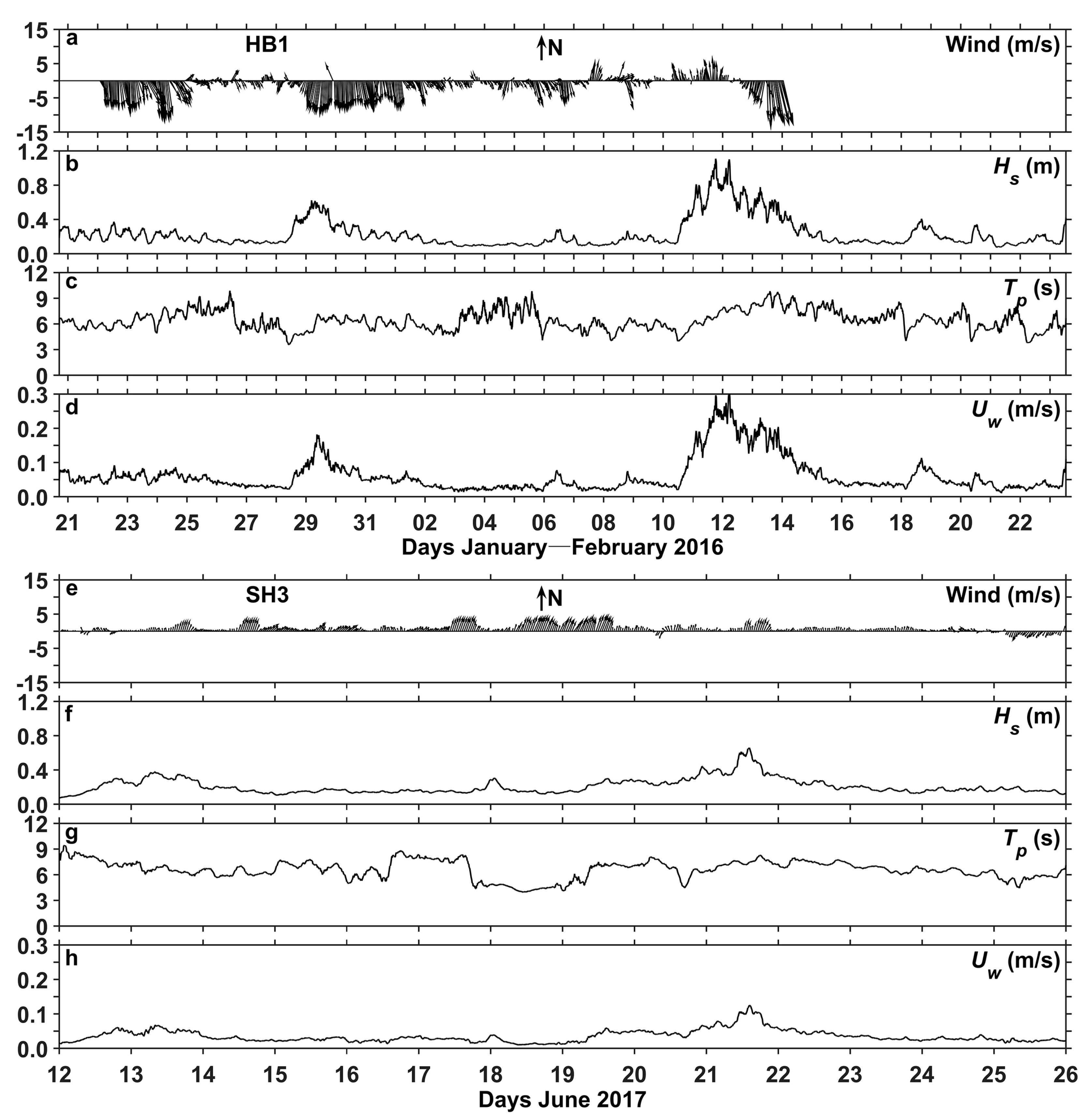
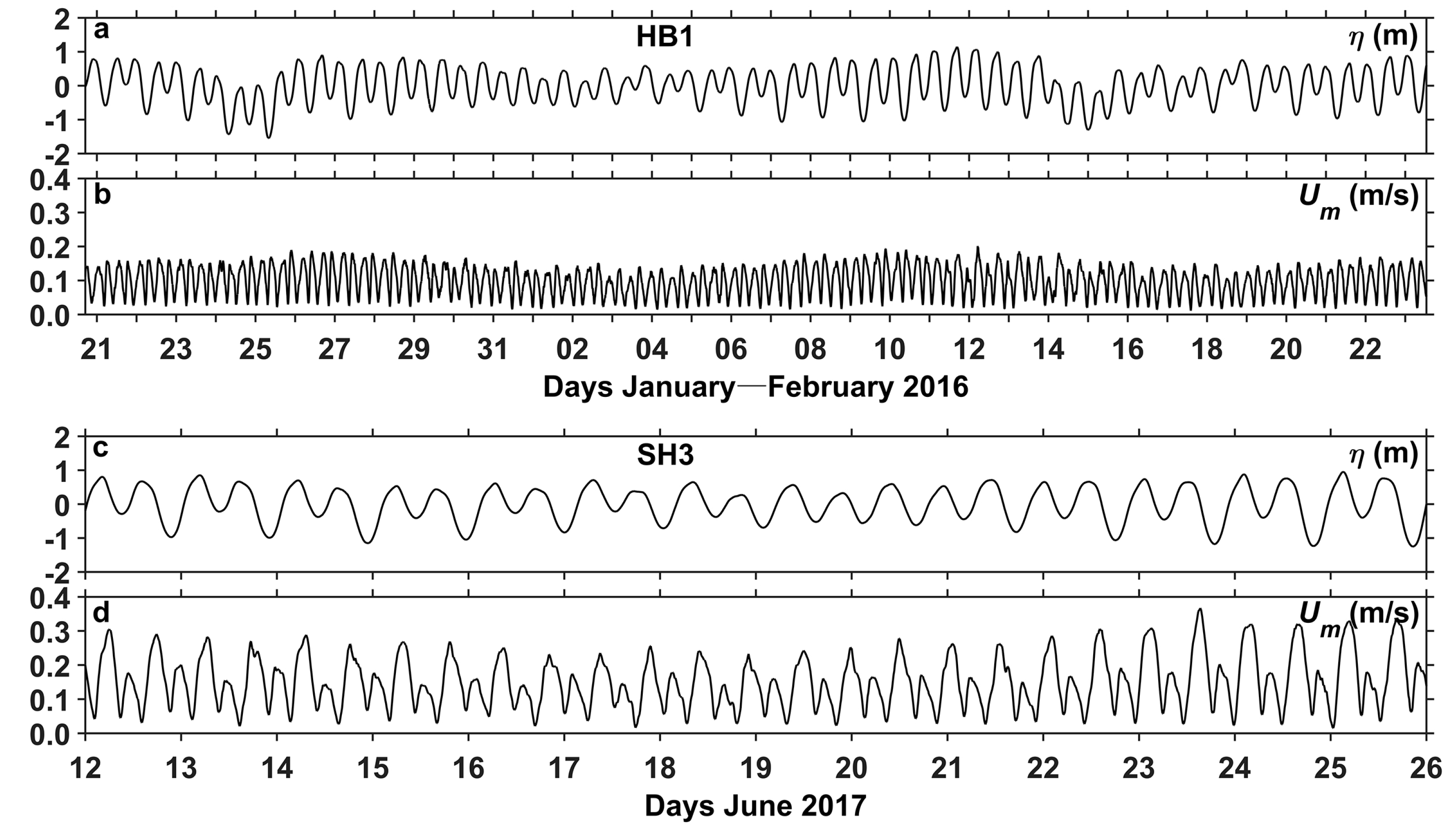
3. Hydrodynamic Conditions

During the winter observations, the north-westerly winds were dominant with $W_{10}$ having a range of 0.1–16.9 m/s and a mean value of 5.0 m/s (Figure 2a). Relatively stronger winds ($W_{10}$ > 10.0 m/s) occurred on 23 January and 13 February; moderate winds (5.0 < $W_{10}$ < 10.0 m/s) appeared from 29 January to 1 February; and weak winds ($W_{10}$ < 5.0 m/s) presented from 26 January to 28 January and from 2 February to 5 February. In summer, the study area was dominated by the southerly winds (Figure 2e), with $W_{10}$ being less than 6.0 m/s and a mean value of 1.7 m/s.

In winter, $H_s$, $T_p$, and $U_w$ were within ranges of 0.08–1.11 m, 3.5–10.1 s, and 0.01–0.31 m/s, respectively (Figure 2b–d). Relatively stronger wave processes ($H_s$ > 0.40 m, $U_w$ > 0.10 m/s) occurred on 28 January and 11 February. In summer, $H_s$, $T_p$, and $U_w$ were within ranges of 0.07–0.65 m, 3.9–9.4 s, and 0.01–0.12 m/s, respectively (Figure 2f–h). Relatively stronger waves with $H_s$ values of 0.30–0.65 m occurred on 13 June and 21 June, and weak waves with $H_s$ < 0.20 m and $U_w$ < 0.06 m/s persisted during the other dates (Figure 2f,h). The values of $L_{wave}$ were within 17–72 m in winter and 20–76 m in summer. The values of the wave steepness (${\delta }_{wave}=H_s/L_{wave}$) were within 0.001–0.023 in winter and 0.001–0.013 in summer. Hence, in both winter and summer the waves did not reach the breaking state because the values of ${\delta }_{wave}$ were less than the critical value of 0.142. Half of $L_{wave}$ was greater than the average water depth, suggesting the influence of waves on the BBL. On the other hand, the thickness of the wave-induced boundary layer is less than 3 cm and 2 cm in winter and summer, respectively, estimated according to $2\pi T_p{u}_{\ast w}$ [51], with $u_{\ast w}$ being the wave-induced friction velocity to be discussed later in Section 5.3.

Waves in the study area may be dominated by either wind waves or swells. In winter, a previous analysis by Fan et al. [52] suggested that the significant variations of $H_s$ were mainly caused by swells. In summer, the relatively larger values of significant wave height ($H_s$ > 0.30 m, Figure 2f) were obtained when winds were weak ($W_{10}$ < 3.0 m/s, Figure 2e) and the average value of $T_p$ was about 6.9 s (Figure 2g), the typical period of swells. This indicates the dominance of swells during the summer observations.

Figure 3 shows the time series of $\eta$ and $U_m$. Variations of $\eta$ had ranges of −1.5–+1.2 m in winter and −1.3–+1.0 m in summer. Significant decreases in $\eta$ occurred when winds were strong, e.g., from January 24 to January 25 and from February 14 to February 15 (Figure 2a and Figure 3a). Variations of $U_m$ had ranges of 0.01–0.20 m/s in winter and 0.02–0.37 m/s in summer. The variations of $\eta$ and $U_m$ were both significantly influenced by the semidiurnal tides. The flow directed westward (eastward) during the flood (ebb) tide, with $u$ being much larger than $v$ (Figure 4). The harmonic analysis is applied to the time series of $\eta$ and velocities. The results suggest that both elevations and currents were dominated by tidal variations, with the M₂ component being the most significant. The duration of flood (ebb) tide was 6.4 (6.0) hours [52].

The variations of $U_m$ showed four peak values per day (Figure 3b,d). In winter, $U_m$ had peak values of about 0.15 m/s during both flood and ebb tides. In summer, the peak values of $U_m$ were about 0.15 m/s during flood tide, much weaker than about 0.30 m/s during ebb tide. This seasonal difference in the characteristics of tidal currents was related to the local raft aquaculture for kelp, as outlined by the green curve in Figure 1. In summer, the cultured kelp were mostly harvested, hence their influence on the currents is expected to be weak. The flood tide is weaker than the ebb tide at SH3, and this is due to the differences in the spatial distributions of the flow between the two phases. That is, the flood tidal flow is distributed more uniformly across the entrance of the bay, while the ebb tidal flow is more concentrated along the northern side where SH3 was located. In winter, the cultured kelp were in growing phases, causing significant resistance to the tidal flow [39,42]. The resistance caused by the kelp aquaculture can affect the flood tidal flow across most areas of the bay, and it may also alter the spatial distribution of the ebb tidal flow to be less concentrated at the site of HB1. This is a plausible explanation for the attenuated ebb tidal flow at HB1 in winter compared with the stronger ebb flow at SH3 in summer.

4. Estimation of Turbulent Parameters

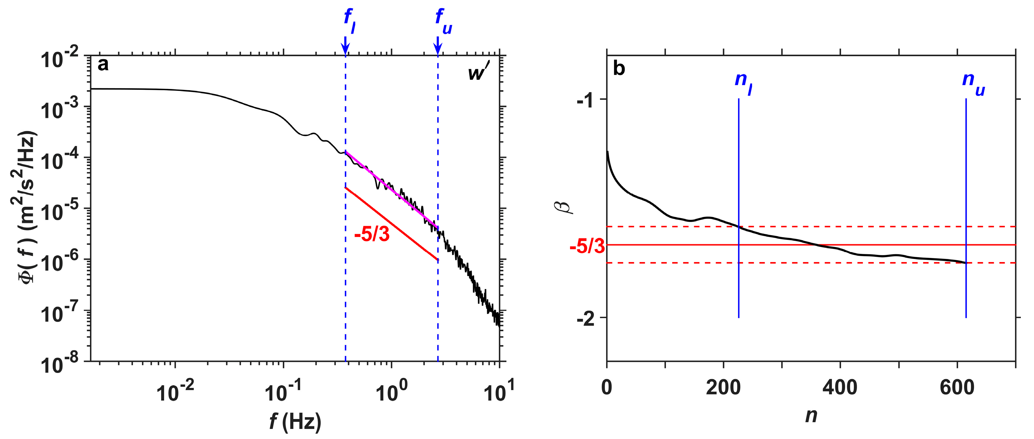
The three velocity components ($u$, $v$, and $w$) measured by the ADV can be decomposed into the mean and fluctuation components. Taking $u$ as an example, we have

$$u=\overline{u}+u^{\prime },$$

(1)

where $\overline{u}$ denotes the mean component averaged over 10 min and $u^{\prime }$ denotes the fluctuation component. With the presence of wave impacts, $u^{\prime }$ can be further decomposed into

$$u^{\prime }=u_w^{\prime }+u_t^{\prime },$$

(2)

where $u_w^{\prime }$ and $u_t^{\prime }$ denote the wave and turbulent components, respectively [25,53,54].

Figure 5 shows the energy spectra $\varphi \left(f\right)$ of velocity fluctuations as a function of frequency $f$ during the phases without and with the presence of significant waves at Station SH3. In the absence of significant waves, the spectra of $u^{\prime }$, $v^{\prime }$, and $w^{\prime }$ (Figure 5a) exhibit obvious inertial subrange characterized by the Kolmogorov “−5/3” law (magenta lines in Figure 5) and are very similar to that in tidal currents [5,27]. In the presence of significant waves with $H_s$ = 0.46 m and $T_p$ = 6.2 s, the spectra of $u^{\prime }$, $v^{\prime }$, and $w^{\prime }$ (solid lines in Figure 5b) show energy peaks at periods of about 6.0 s, corresponding to the wave peak period. This indicates the existence of the wave signals in velocity fluctuations.

In order to estimate TKE and TRS, the wave signals need to be separated from the velocity fluctuations through wave-turbulence decomposition. Existing decomposition methods are based on analyses of the co-spectra [55,56], coherence [57], empirical mode decomposition [58], and synchro-squeezed wavelet transform (SWT) [59,60]. Bian et al. [25] evaluated the performances of the above four methods and demonstrated the advantages of using the SWT method. Evolving from the wavelet transform algorithm and the reallocation method, the SWT method decomposes nonlinear and nonstationary signals into a number of components in the time–frequency plane and can effectively extract the independent components [59,60]. Figure 6 demonstrates the key steps of wave-turbulence decomposition using the SWT method for velocity fluctuations in the presence of wave impacts. The raw velocity fluctuations (black line in Figure 6a,c) are decomposed into a number of modes. The second mode captures the main variations of the wave motions (red line in Figure 6a,c) and the rest of the modes constitute parts of the turbulent fluctuations (blue lines in Figure 6a,c). The time series of velocity fluctuations for the wave and turbulent components are obtained through recombining the decomposed modes (Figure 6b,d). The dashed line in Figure 5b shows the resulting spectrum of the turbulent fluctuations after removing the wave component, similar to the spectrum in the absence of wave impacts (Figure 5a).

After obtaining the turbulent fluctuations, TKE and TRS are calculated according to

$$TKE=\left(\overline{u_t^{\prime }{}^2}+\overline{v_t^{\prime }{}^2}+\overline{w_t^{\prime }{}^2}\right)/2,$$

(3)

$$TRS={\left[{\left(-\overline{u_t^{\prime }{w}_t^{\prime }}\right)}^2+{\left(-\overline{v_t^{\prime }{w}_t^{\prime }}\right)}^2\right]}^{0.5},$$

(4)

where the overbar denotes averaging over 10 min.

For well-developed turbulence, $\epsilon$ can be estimated based on the spectra of velocity fluctuations in the inertial subrange characterized by the Kolmogorov “−5/3” law, i.e.,

$$\varphi \left(f\right)={\left(U_m/2\pi \right)}^{2/3}\alpha {\epsilon }^{2/3}{f}^{-5/3},$$

(5)

or in logarithmic form as

$${\log }_{10}\left[\varphi \left(f\right)\right]=-5/3{\log }_{10}\left(f\right)+{\log }_{10}\left\{\left[{\left(U_m/2\pi \right)}^{2/3}\alpha {\epsilon }^{2/3}\right]\right\},$$

(6)

where $\varphi \left(f\right)$ is the spectral density in frequency ($f$) space, and $\alpha$ is the one-dimensional Kolmogorov universal constant [61]. Previous studies have successfully applied this method to estimate $\epsilon$ using the spectra of raw $w^{\prime }$ in conditions of weak wave influence [26,62,63]. We now follow this approach to fit a spectrum of observed $w^{\prime }$ to

$${\log }_{10}\left[\varphi \left(f\right)\right]=\beta {\log }_{10}\left(f\right)+\gamma ,$$

(7)

where $\beta$ and γ are fitting parameters. In the inertial subrange $\beta$ = −5/3, then $\epsilon$ is calculated according to

$$\epsilon ={\left({10}^{\gamma }/\alpha \right)}^{3/2}\left(2\pi /U_m\right).$$

(8)

The key to estimating $\epsilon$ using this method is to find the range of ${\log }_{10}\left(f\right)$ for an observed spectrum where $\beta$ is statistically close to −5/3. In previous studies, the inertial subrange was mostly identified by visually examining each individual spectrum. This is not efficient if a large number of spectra need to be processed. Here, we propose an iterative fitting procedure to objectively identify the inertial subrange. This procedure includes the two following steps.

• For a spectrum of observed $w^{\prime }$, the first step is to find the low-frequency bound of the inertial subrange, denoted as $f_l$. The fit of the spectrum to Equation (7) is tried successively over a frequency range from $f_o+\left(n-1\right)\delta f$ to $f_o+\left(n-1\right)\delta f+\Delta f$, where $n$ is the number of the trial fit, $f_o$ is the lowest resolved frequency of the spectrum, and $\delta f$ and $\Delta f$ are the prescribed frequency increment and frequency range of each trial fit. We set $\Delta f$ = 1.6 Hz, which is smaller than the expected frequency range of the inertial subrange, and $\delta f$ = 1.7 × 10⁻³ Hz, which is fine enough to resolve the frequency range $\Delta f$. This is equivalent to applying the fitting over a “sliding window” of width $\Delta f$ in the frequency axis, starting from the lowest frequency end $f_o$, and each trial shifts to a higher frequency by an increment $\delta f$. Each trial fit obtains a value of $\beta$, which is checked against the 5% bound of −5/3. As the value of $n$ increases, a value of $\beta$ will fall within this bound if the inertial subrange exists. For the lowest value of $n$, denoted as $n_l$, that satisfies this condition, we set $f_l=f_o+\left(n_l-1\right)\delta f$.
• The second step is to find the upper frequency bound of the inertial subrange, denoted as $f_u$. In this case, the successive least squares fittings are tried for frequency ranges from $f_l$ to $f_l+\Delta f+\left(n-n_l\right)\delta f$. That is, the trial fittings are applied to a frequency window starting from $f_l$ but with window width increasing by $\delta f$ as $n$ increases. The values of $\beta$ are checked against the 5% bound of −5/3. Initially, the $\beta$ value for each trial fitting is within this bound. For the lowest value of $n$, denoted as $n_u$, that satisfies this condition, we set $f_u=f_o+\left(n_u-n_l\right)\delta f$.

As an example, Figure 7a shows an example of a spectrum with $f_l$ and $f_u$ identified using the above procedure, and Figure 7b shows the values of $\beta$ as a function of the trial number $n$ of the least squares fitting. The value of $\beta$ for the fitting in the identified inertial subrange (frequency from $f_l$ to $f_u$) is used to calculate $\epsilon$, according to Equation (8).

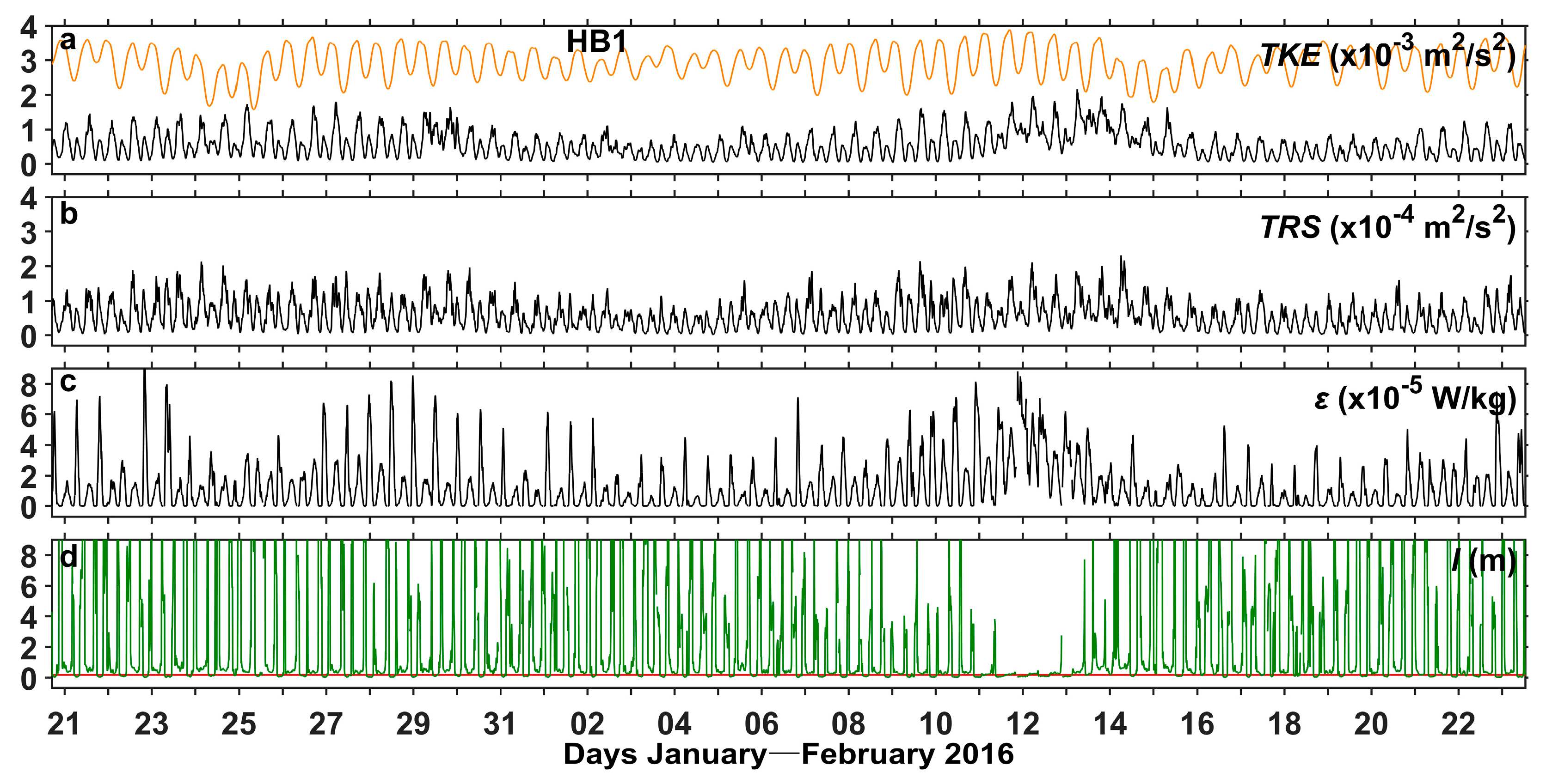
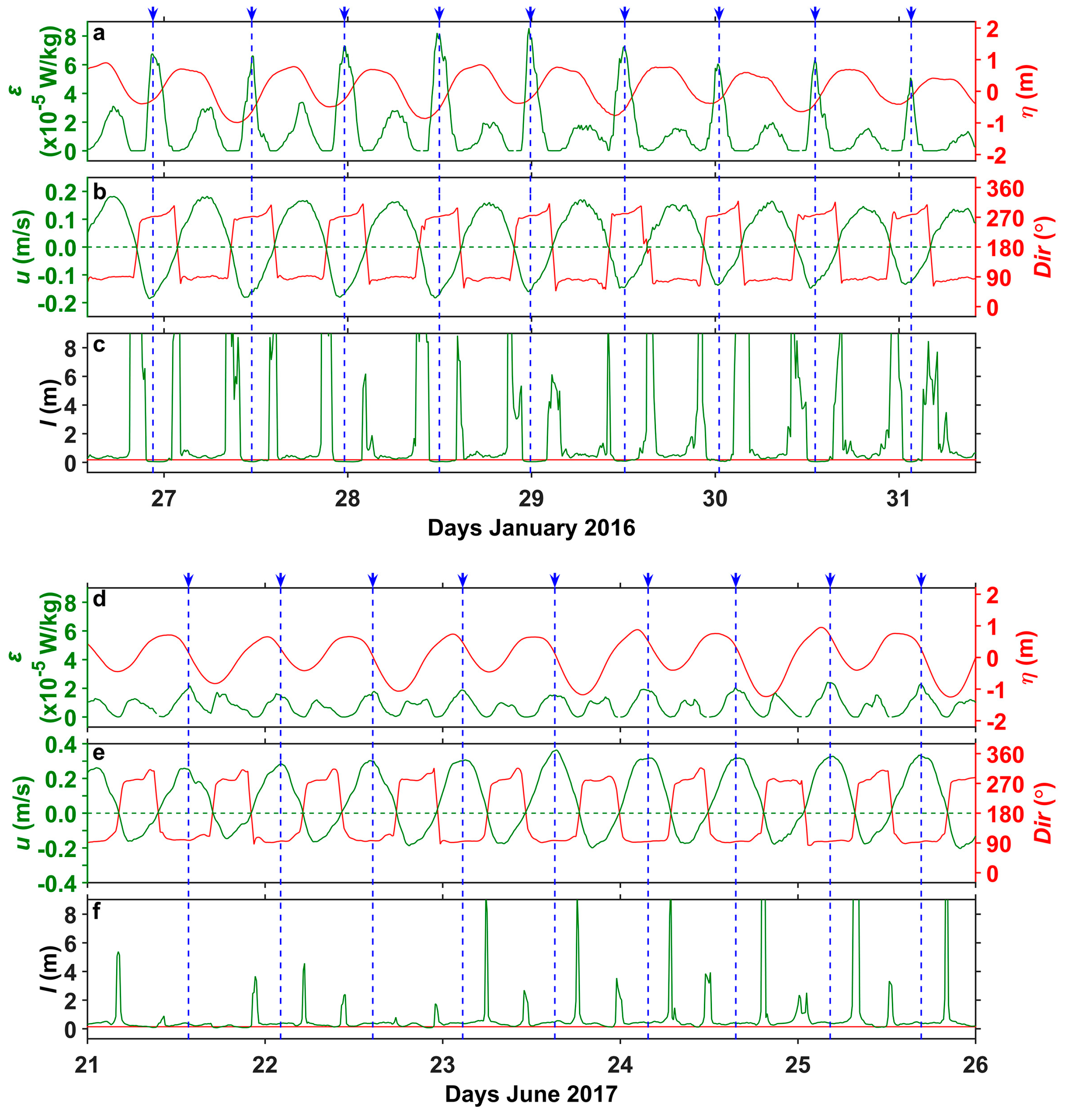
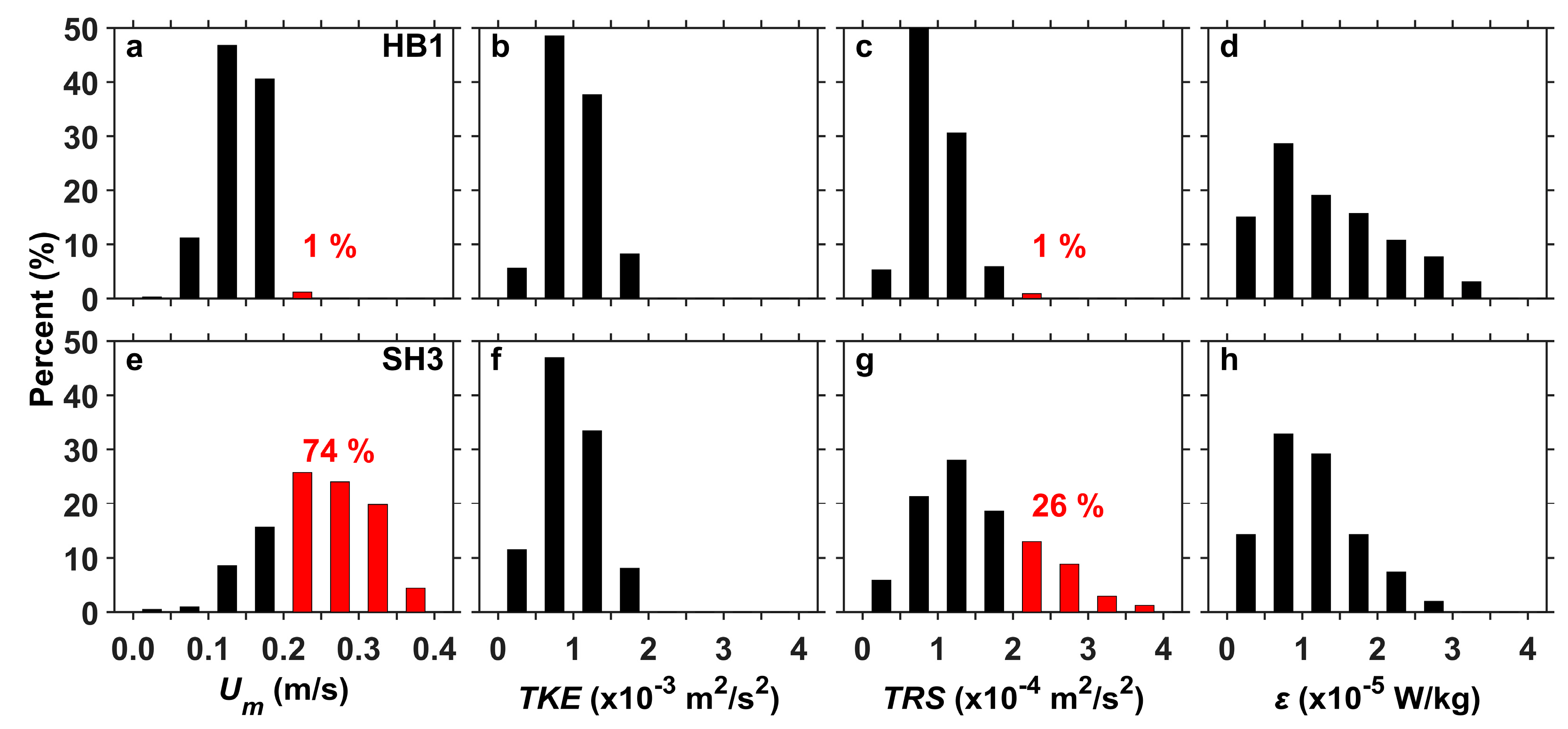
5. Variations of Estimated Turbulent Parameters

5.1. Variations of TKE, TRS, and $\epsilon$

Because the influence of kelp culture did not present in summer, the time variations of TKE, TRS, and $\epsilon$ in the BBL for this season are first presented (Figure 8a–c). The three quantities vary in the ranges of 3.4 × 10⁻⁵–1.5 × 10⁻³ m²/s², 2.0 × 10⁻⁶–3.5 × 10⁻⁴ m²/s², and 1.3 × 10⁻⁸–2.4 × 10⁻⁵ W/kg, with time-mean values of 4.8 × 10⁻⁴ m²/s², 7.5 × 10⁻⁵ m²/s², and 6.1 × 10⁻⁶ W/kg, respectively. The three quantities show evident semidiurnal tidal signals, with relatively larger values during the stronger ebb flow than during the weaker flood flow.

During the winter observations with the presence of the kelp culture influences, the time variations of TKE, TRS, and $\epsilon$ are presented in Figure 9a–c. The three quantities vary in the ranges of 4.0 × 10⁻⁵–2.2 × 10⁻³ m²/s², 1.6 × 10⁻⁶–2.3 × 10⁻⁴ m²/s², and 7.2 × 10⁻⁹–1.0 × 10⁻⁴ W/kg, with time-mean values of 5.6 × 10⁻⁴ m²/s², 5.9 × 10⁻⁵ m²/s², and 1.2 × 10⁻⁵ W/kg, respectively. TKE and TRS are both slightly stronger during ebb than during flood tides. During flood tide, $\epsilon$ shows larger peak values in the range of 4.0 × 10⁻⁵–8.0 × 10⁻⁵ W/kg, compared with the peak values of $\epsilon$ during ebb in the range of 1.0 × 10⁻⁵–2.0 × 10⁻⁵ W/kg.

From a zoom-in segment of the time series of $\epsilon$, flow, and sea level in winter (Figure 10a,b), large values of $\epsilon$ are obtained during the strong westward flood tidal flow with the peaks occurring soon after the flood tidal flow reaching the maximum. For the summer season (Figure 10d,e), relatively large values of 𝜀 are present during the strong eastward ebb tidal flow.

As discussed in Section 3, the presence of kelp culture can influence the variations of tidal currents in winter. Thus, we expect to see different characteristics of the variations of turbulent parameters during the ebb tidal flows between summer and winter, as presented by the histograms of $U_m$, TKE, TRS, and $\epsilon$ in Figure 11. In summer, without the presence of kelp aquaculture at Station SH3, 74% of the ebb flow speed has values $U_m$ > 0.20 m/s and 26% of the Reynolds stress has values TRS > 2.0 × 10⁻⁴ m²/s²; while, in winter at Station HB1, during ebb, only about 1% of the flow speed and Reynolds stress have values $U_m$ > 0.20 m/s and TRS > 2.0 × 10⁻⁴ m²/s², respectively. On the other hand, TKE and $\epsilon$ do not show significant difference between the conditions with and without the presence of kelp aquaculture during the ebb. In Section 5.3, we will discuss why during the ebb in winter $U_m$ and TRS are significantly reduced while TKE and $\epsilon$ are not.

According to the turbulent closure model proposed by Mellor and Yamada [64,65], a master length scale ($l$) can be computed by

$$l=q^3/\left(B_1\epsilon \right),$$

(9)

where $q$ is related to TKE = $q^2$/2, and $B_1$ is an empirical parameter. In unstratified flow $B_1$ = 16.6; Lu et al. [66] suggested that $B_1$ > 16.6 in weakly stratified tidal flow. Figure 8d and Figure 9d show the time series of $l$ (green) in comparison with the mixing length $l_m=\kappa z$ (red) in the classical wall-bounded turbulent boundary layer, where $\kappa$ = 0.40 is the von Karman constant and $z$ is the distance from the wall (height above the seafloor). During both summer and winter, the values of $l$ are close to $\kappa z$ except during the turning of the tidal flow from ebb to flood or vice versa (Figure 8d, Figure 9d, Figure 10c,f).

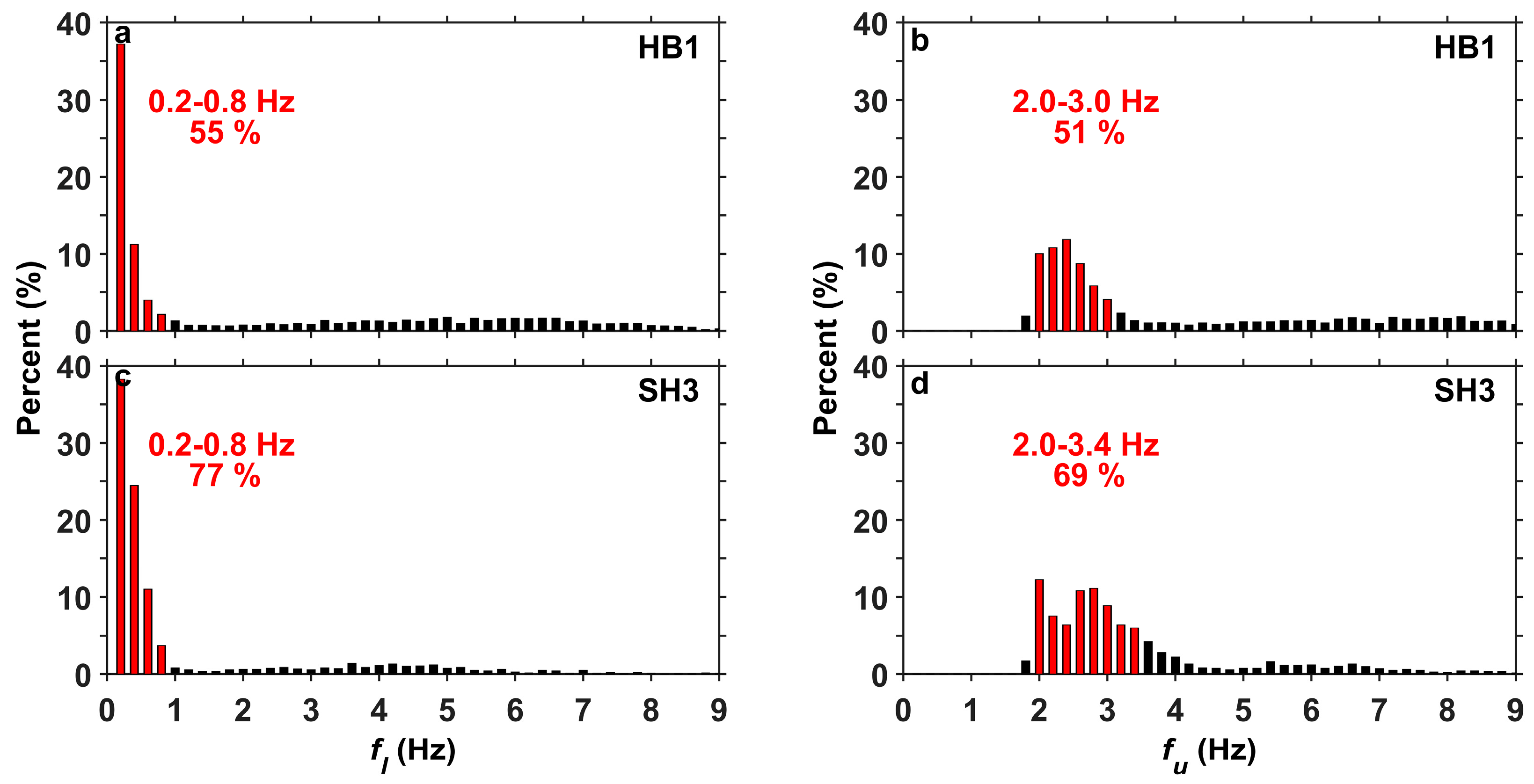
5.2. Variation of the Inertial Subrange

The lower and upper frequency bounds of the inertial subrange ($f_l$ and $f_u$) identified from the least squares fitting procedure are not constant. Figure 12 shows the histograms of $f_l$ and $f_u$ for the winter and summer observations separately. The majority values of $f_l$ are within 0.2–0.8 Hz, accounting for 55% and 77% in winter and summer, respectively. The majority values of $f_u$ are within 2.0–3.0 Hz in winter and 2.0–3.4 Hz in summer, accounting for 51% and 69%, respectively.

The frequency bounds $f_l$ and $f_u$ can be converted to wavenumber bounds according to $k_l=f_l/U_m$ and $k_u=f_u/U_m$. Can the variations of $k_l$ and $k_u$ be related to $U_m$, TKE, and $\epsilon$? According to the scatter diagrams presented in Figure 13, the relationships in winter and summer are similar, with both $k_l$ and $k_u$ decreasing with increasing $U_m$, TKE, and $\epsilon$. Figure 13 also shows that for each range of $U_m$, TKE, or $\epsilon$, the standard deviations of $k_u$ and $k_l$ usually overlap. This is due to the large scattering in the values of $k_u$ and $k_l$ and the relatively small number of data samples (inertial subranges identified) with the current data sets. The wavelength where the inertial subrange is present, denoted as $L_{sub}$, can be calculated as $1/\left(k_u-k_l\right)$. For weak flows of $U_m$ < 0.05 m/s, $L_{sub}$ has smaller values of 6.25 × 10⁻³–1.25 × 10⁻² m; for strong flows of $U_m$~0.20–0.35 m/s, $L_{sub}$ increases to 0.07–0.83 m. With respect to the ranges of $\epsilon$ values of 10⁻⁸–10⁻⁷, 10⁻⁷–10⁻⁶, 10⁻⁶–10⁻⁵, and 10⁻⁵–10⁻⁴ W/kg, $L_{sub}$ has values of 7.75 × 10⁻³–1.42 × 10⁻², 1.01 × 10⁻²–1.74 × 10⁻², 1.74 × 10⁻²–1.47 × 10⁻¹, and 3.70 × 10⁻²–4.16 × 10⁻¹ m, respectively.

Variations in the frequency and wavenumber bounds and also the wavelength for the inertial subrange, as identified in the above, have implications on the sampling strategy in field observations. According to our data, the majority values of the upper frequency bound $f_u$ are less than 4 Hz (Figure 12); thus, a sampling rate of 8 Hz would be sufficient to resolve the inertial subrange. For strong flows of $U_m$~0.20–0.35 m/s, $L_{sub}$ is in the range of 0.07–0.83 m. This suggests that setting the smaller bin size for non-pointwise instruments may resolve most of the inertial subrange spectra. The bin size needs to be further refined for weak flows with smaller TKE intensity and dissipation.

5.3. Comparing the TKE Dissipation Rate with the Estimated Production Rate

In the turbulent boundary layer, $\epsilon$ and the production rate ($P$) are the two dominate terms in the TKE budget, and, in unstratified flows, the local balance between the two terms, i.e., $P=\epsilon$, usually holds [27,66]. In the study site, the synthesis results of observed water temperature and salinity did not show the conditions of stratification in both winter and summer (figure omitted). In the present analysis, the estimated $\epsilon$ through fitting the observed spectra in the inertial subrange can be taken as the total rate of TKE dissipation (subject to the assumptions of the theory). However, for the TKE production rate, the ADV measurement only provided partial information to estimate the contributions related to the vertical shear, i.e., $P_t$ and $P_w$ which represent the action of mean vertical flow shear against TSR and wave stress, respectively.

The calculation of $P_w$ follows, e.g., Reynolds and Hussain [67] and Egan et al. [68]. Along the mean flow direction, the shear is denoted as $\partial U_m/\partial z$, and the magnitude of TRS and wave stress as $u_{\ast t}^2$ and $u_{\ast w}^2$; then,

$$P_t=u_{\ast t}^2\left(\partial U_m/\partial z\right),$$

(10)

$$P_w=u_{\ast w}^2\left(\partial U_m/\partial z\right),$$

(11)

where $u_{\ast w}^2={\left[{\left(-\overline{u_w^{\prime }{w}_w^{\prime }}\right)}^2+{\left(-\overline{v_w^{\prime }{w}_w^{\prime }}\right)}^2\right]}^{0.5}$. Here, we calculate $\partial U_m/\partial z$ based on classical BBL theory. That is, near the boundary, there exists a “logarithmic layer” in terms of the velocity distribution, TRS has a constant profile, the turbulent mixing length is $l_m=\kappa z$, and the velocity shear can be expressed as

$$\partial U_m/\partial z=u_{\ast t}/\kappa z.$$

(12)

Using Equation (12) to compute the flow shear, we need to examine how well $l_m=\kappa z$ applies to our data. The turbulent mixing length can be related to the master length scale $l$ in the Mellor–Yamada turbulent closure model [66]. Based on the comparison between $\kappa z$ and $l$ presented in Section 5.1, we select the analyzed data segments with $l$ being close to $\kappa z$.

Based on the above equations, the production rates $P_t$ and $P_w$ are calculated. Figure 14 shows the scatter diagram of $\epsilon$ versus $P_t$ and $P_t$ + $P_w$, split into four cases, i.e., for flood and ebb tidal flows during summer and winter, separately. First, $P_t$ is, on average, larger than $P_w$. Secondly, with the wave impacts included, the magnitudes of $\epsilon$ and $P_t+P_w$ are closer to each other. In summer at SH3, $P_t+P_w$ is, on average, close to $\epsilon$ during both the flood and ebb tidal flows (Figure 14c,d). During the ebb flow in winter, $\epsilon$ is, on average, close but slightly larger than $P_t+P_w$ (Figure 14b). During the flood flow in winter, $\epsilon$ is, on average, close to $P_t+P_w$ except for these episodes of larger spike values of $\epsilon$ (Figure 14a, solid circles). Finally, $\epsilon$ is larger than $P_t+P_w$ during the peculiar large values of $\epsilon$ in winter (Figure 14a, hollow squares). The imbalance between $\epsilon$ and $P_t+P_w$ in winter suggests that the presence of heavy kelp aquaculture causes reduction in TKE production related to the vertical shear while increasing the horizontal shear and its contribution to TKE production. This provides a reasonable explanation for the high level of TKE and of $\epsilon$ under the much-reduced tidal flow and TRS in winter. Unfortunately, the horizontal shear was not measured in our field work.

6. Conclusions

This study analyzes high-frequency measurements with the bottom-mounted ADV in the bottom boundary layer of a shallow bay. The synchro-squeezed wavelet transform is applied for wave-turbulence decomposition, and an iterative procedure is developed to identify of the turbulence inertial subrange. Time series of flow, wave characteristics, and turbulence parameters are derived for both the winter and summer seasons. The main results are summarized below.

The frequency and wavenumber ranges of the inertial subrange are not constant. The majority values of low- and high-frequency bounds are within 0.2–0.8 Hz and 2.0–3.0 Hz, respectively. The corresponding upper and lower wavenumber bounds both decrease with the increasing flow speed, TKE, and $\epsilon$. The wavelength of the inertial subrange increases with the increasing mean flow. This result is expected because stronger mean flow means more separation between the energy-containing scales and dissipation scales—thereby causing a larger inertial range. Or, conversely, if the mean flow decreases, then the inertial range decreases. The wavelength of the inertial subrange has smaller values of 6.25 × 10⁻³–1.25 × 10⁻² m for weak flows of $U_m$ < 0.05 m/s, and increases to 0.07–0.83 m for strong flows of $U_m$~0.20–0.35 m/s. This has implications on the sampling requirement of non-pointwise instruments in order to resolve the inertial subrange, i.e., a sampling rate of 8 Hz or higher, and a smaller bin size.

The flood-ebb tidal flows and turbulent parameters show different variations between the summer and winter seasons. Without the presence of kelp aquaculture in summer, the flow is stronger during ebb than during flood at the observational site, and $\epsilon$, TKE, and TRS increase smoothly with the increasing tidal flow magnitude. TKE dissipation is approximately in balance with the production rate due to the action of vertical shear against TRS and wave stress. With the presence of heavy kelp aquaculture in winter, the flood tidal flow is not attenuated and TKE and TRS have similar magnitudes, while $\epsilon$ shows larger spike values in comparison with summer. In winter, the ebb tidal flow and TRS are both attenuated, while $\epsilon$ and TKE have similar values, in comparison with summer. During both flood and ebb tidal flows in winter, TKE dissipation can be significantly larger than the production related to the vertical shear. A plausible explanation is that the presence of kelp aquaculture induces large horizontal shear and its contribution to TKE production, which are unfortunately not measured in our field work.

The summer and winter observation stations are quite close, so the above results are effectively derived from a single-point measurement. While this allows revealing the difference in variations between summer and winter, future observations should quantify the horizontal variations of flow and turbulence due to the kelp aquaculture.

References

1. Wang, Y.; Voulgaris, G.; Li, Y.; Yang, Y.; Gao, J.; Chen, J.; Gao, S. Sediment resuspension, flocculation, and settling in a macrotidal estuary. J. Geophys. Res. Oceans 2013, 118, 5591–5608. [Google Scholar] [CrossRef]
2. Yang, Y.; Gao, S.; Wang, Y.; Jia, J.; Xiong, J.; Zhou, L. Revisiting the problem of sediment motion threshold. Cont. Shelf Res. 2019, 187, 103960. [Google Scholar] [CrossRef]
3. Yang, Y.; Wang, Y.; Gao, S.; Wang, X.; Shi, B.; Zhou, L.; Wang, D.; Dai, C.; Li, G. Sediment resuspension in tidally dominated coastal environments: New insights into the threshold for initial movement. Ocean Dynam. 2016, 66, 401–417. [Google Scholar] [CrossRef]
4. Yuan, Y.; Wei, H.; Zhao, L.; Cao, Y. Implications of intermittent turbulent bursts for sediment resuspension in a coastal bottom boundary: A field study in the western Yellow Sea, China. Mar. Geol. 2009, 263, 87–96. [Google Scholar] [CrossRef]
5. Yuan, Y.; Wei, H.; Zhao, L.; Jiang, W. Observations of sediment resuspension and settling off the mouth of Jiaozhou Bay, Yellow Sea. Cont. Shelf Res. 2008, 28, 2630–2643. [Google Scholar] [CrossRef]
6. Wang, J.; Wei, H.; Lu, Y.; Zhao, L. Diffusive boundary layer influenced by bottom boundary hydrodynamics in tidal flows. J. Geophys. Res. Oceans 2013, 118, 5994–6005. [Google Scholar] [CrossRef]
7. Wang, J.; Zhao, L.; Fan, R.; Wei, H. Scaling relationships for diffusive boundary layer thickness and diffusive flux based on in situ measurements in coastal seas. Prog. Oceanogr. 2016, 144, 1–14. [Google Scholar] [CrossRef]
8. Rippeth, T.P.; Fisher, N.R.; Simpson, J.H. The cycle of turbulent dissipation in the presence of tidal straining. J. Phys. Oceanogr. 2001, 31, 2458–2471. [Google Scholar] [CrossRef]
9. Thorpe, S.A.; Green, J.A.M.; Simpson, J.H.; Osborn, T.R.; Nimmo Smith, W.A.M. Boils and turbulence in a weakly stratified shallow tidal sea. J. Phys. Oceanogr. 2008, 38, 1711–1730. [Google Scholar] [CrossRef]
10. Cui, Y.; Wu, J.; Qiu, C. Enhanced mixing by patchy turbulence in the northern South China Sea. Cont. Shelf Res. 2018, 166, 34–43. [Google Scholar] [CrossRef]
11. Lozovatsky, I.D.; Fernando, H.J.S.; Planella-Morato, J.; Liu, Z.; Lee, J.H.; Jinadasa, S.U.P. Probability distribution of turbulent kinetic energy dissipation rate in ocean: Observations and approximations. J. Geophys. Res. Oceans 2017, 122, 8293–8308. [Google Scholar] [CrossRef]
12. Lozovatsky, I.D.; Liu, Z.; Fernando, H.J.S.; Hu, J.; Wei, H. The TKE dissipation rate in the northern South China Sea. Ocean Dynam. 2013, 63, 1189–1201. [Google Scholar] [CrossRef]
13. Lozovatsky, I.D.; Shearman, K.; Pirro, A.; Fernando, H.J.S. Probability distribution of turbulent kinetic energy dissipation rate in stratified turbulence: Microstructure measurements in the Southern California Bight. J. Geophys. Res. Oceans 2019, 124, 4591–4604. [Google Scholar] [CrossRef]
14. Hackett, E.E.; Luznik, L.; Nayak, A.R.; Katz, J.; Osborn, T.R. Field measurements of turbulence at an unstable interface between current and wave bottom boundary layers. J. Geophys. Res. Oceans 2011, 116, C02022. [Google Scholar] [CrossRef] [Green Version]
15. Lu, Y.; Lueck, R.G. Using a broadband ADCP in a tidal channel Part II: Turbulence. J. Atmos. Ocean. Tech. 1999, 16, 1568–1579. [Google Scholar] [CrossRef]
16. Rippeth, T.P.; Williams, E.; Simpson, J.H. Reynolds stress and turbulent energy production in a tidal channel. J. Phys. Oceanogr. 2002, 32, 1242–1251. [Google Scholar] [CrossRef]
17. Souza, A.J.; Alvarez, L.G.; Dickey, T.D. Tidally induced turbulence and suspended sediment. Geophys. Res. Lett. 2004, 31, L20309. [Google Scholar] [CrossRef] [Green Version]
18. Stacey, M.T.; Monismith, S.G.; Burau, J.R. Measurements of Reynolds stress profiles in unstratified tidal flow. J. Geophys. Res. Oceans 1999, 104, 10933–10949. [Google Scholar] [CrossRef]
19. Lucas, N.S.; Simpson, J.H.; Rippeth, T.P.; Old, C.P. Measuring turbulent dissipation using a tethered ADCP. J. Atmos. Ocean. Tech. 2014, 31, 1826–1837. [Google Scholar] [CrossRef] [Green Version]
20. Mcmillan, J.M.; Hay, A.E. Spectral and structure function estimates of turbulence dissipation rates in a high-flow tidal channel using broadband ADCPs. J. Atmos. Ocean. Tech. 2017, 34, 5–20. [Google Scholar] [CrossRef]
21. Mohrholz, V.; Prandke, H.; Lass, H.U. Estimation of TKE dissipation rates in dense bottom plumes using a pulse coherent acoustic Doppler profiler (PC-ADP)—Structure function approach. J. Marine Syst. 2008, 70, 217–239. [Google Scholar] [CrossRef]
22. Wiles, P.J.; Rippeth, T.P.; Simpson, J.H.; Hendricks, P.J. A novel technique for measuring the rate of turbulent dissipation in the marine environment. Geophys. Res. Lett. 2006, 33, L21608. [Google Scholar] [CrossRef]
23. Hackett, E.E.; Luznik, L.; Katz, J.; Osborn, T.R. Effect of finite spatial resolution on the turbulent energy spectrum measured in the coastal ocean bottom boundary layer. J. Atmos. Ocean. Tech. 2009, 26, 2610–2625. [Google Scholar] [CrossRef] [Green Version]
24. Amirshahi, S.M.; Kwoll, E.; Winter, C. Near bed suspended sediment flux by single turbulent events. Cont. Shelf Res. 2018, 152, 76–86. [Google Scholar] [CrossRef]
25. Bian, C.; Liu, Z.; Huang, Y.; Zhao, L.; Jiang, W. On estimating turbulent Reynolds stress in wavy aquatic environment. J. Geophys. Res. Oceans 2018, 123, 3060–3071. [Google Scholar] [CrossRef]
26. Liu, Z.; Wei, H. Estimation to the turbulent kinetic energy dissipation rate and bottom shear stress in the tidal bottom boundary layer of the Yellow Sea. Prog. Nat. Sci. 2007, 17, 289–297. [Google Scholar]
27. Lozovatsky, I.D.; Liu, Z.; Wei, H.; Fernando, H.J.S. Tides and mixing in the northwestern East China Sea, Part II: Near-bottom turbulence. Cont. Shelf Res. 2008, 28, 338–350. [Google Scholar] [CrossRef]
28. Tu, J.; Fan, D.; Zhang, Y.; Voulgaris, G. Turbulence, sediment-induced stratification, and mixing under macrotidal estuarine conditions (Qiantang Estuary, China). J. Geophys. Res. Oceans 2019, 124, 4058–4077. [Google Scholar] [CrossRef]
29. Drost, E.J.F.; Lowe, R.J.; Ivey, G.N.; Jones, N.L. Wave-current interactions in the continental shelf bottom boundary layer of the Australian North West Shelf during tropical cyclone conditions. Cont. Shelf Res. 2018, 165, 78–92. [Google Scholar] [CrossRef]
30. Grant, W.D.; Madsen, O.S. Combined wave and current interaction with a rough bottom. J. Geophys. Res. Oceans 1979, 84, 1797–1808. [Google Scholar] [CrossRef]
31. Green, M.O.; Rees, J.M.; Pearson, N.D. Evidence for the influence of wave-current interaction in a tidal boundary layer. J. Geophys. Res. Oceans 1990, 95, 9629–9644. [Google Scholar] [CrossRef]
32. Rosales, P.; Ocampo-Torres, F.J.; Osuna, P.; Monbaliu, J.; Padilla-Hernandez, R. Wave-current interaction in coastal waters: Effects on the bottom-shear stress. J. Marine Syst. 2008, 71, 131–148. [Google Scholar] [CrossRef]
33. Soulsby, R.L.; Hamm, L.; Klopman, G.; Myrhaug, D.; Simons, R.R.; Thomas, G.P. Wave-current interaction within and outside the bottom boundary layer. Coast. Eng. 1993, 21, 41–69. [Google Scholar] [CrossRef]
34. Zhang, H.; Madsen, O.S.; Sannasiraj, S.A.; Chan, E.S. Hydrodynamic model with wave-current interaction in coastal regions. Estuar. Coast. Shelf Sci. 2004, 61, 317–324. [Google Scholar] [CrossRef] [Green Version]
35. MacVean, L.J.; Lacy, J.R. Interactions between waves, sediment, and turbulence on a shallow estuarine mudflat. J. Geophys. Res. Oceans 2014, 119, 1534–1553. [Google Scholar] [CrossRef]
36. Trowbridge, J.H.; Geyer, W.R.; Bowen, M.M.; Williams, A.J., III. Near-bottom turbulence measurements in a partially mixed estuary: Turbulent energy balance, velocity structure, and along-channel momentum balance. J. Phys. Oceanogr. 1999, 29, 3056–3072. [Google Scholar] [CrossRef]
37. Scully, M.E.; Friedrichs, C.T. The influence of asymmetries in overlying stratification on near-bed turbulence and sediment suspension in a partially mixed estuary. Ocean Dynam. 2003, 53, 208–219. [Google Scholar] [CrossRef]
38. Wang, J.; Greenan, B.J.W.; Lu, Y.; Oakey, N.S.; Shaw, W.J. Layered mixing on the New England Shelf in summer. J. Geophys. Res. Oceans 2014, 119, 5776–5796. [Google Scholar] [CrossRef] [Green Version]
39. Fan, X.; Wei, H.; Yuan, Y.; Zhao, L. Vertical structure of tidal current in a typically coastal raft-culture area. Cont. Shelf Res. 2009, 29, 2345–2357. [Google Scholar] [CrossRef]
40. Jackson, G.A.; Winant, C.D. Effect of a kelp forest on coastal currents. Cont. Shelf Res. 1983, 2, 75–80. [Google Scholar] [CrossRef]
41. Rosman, J.H.; Koseff, J.R.; Monismith, S.G.; Grover, J. A field investigation into the effects of a kelp forest (Macrocystis pyrifera) on coastal hydrodynamics and transport. J. Geophys. Res. Oceans 2007, 112, C02016. [Google Scholar] [CrossRef] [Green Version]
42. Shi, J.; Wei, H.; Zhao, L.; Yuan, Y.; Fang, J.; Zhang, J. A physical-biological coupled aquaculture model for a suspended aquaculture area of China. Aquaculture 2011, 318, 412–424. [Google Scholar] [CrossRef]
43. Stevens, C.L.; Petersen, J.K. Turbulent, stratified flow through a suspended shellfish canopy: Implications for mussel farm design. Aquacult. Env. Interac. 2011, 2, 87–104. [Google Scholar] [CrossRef] [Green Version]
44. Xu, P.; Zhang, S.; Cai, H.; Chen, W.; Huang, H.; Liu, C. Characteristics of vertical mixing in a sea-cage farm and its environmental influences in a strong tide system: A case study in the Nanji Archipelago, East China Sea. Aquaculture 2019, 512, 734344. [Google Scholar] [CrossRef]
45. Liu, Y.; Huang, H.; Yan, L.; Liu, X.; Zhang, Z. Influence of suspended kelp culture on seabed sediment composition in Heini Bay, China. Estuar. Coast. Shelf Sci. 2016, 181, 39–50. [Google Scholar] [CrossRef]
46. Zhu, Z.; Hu, Z.; Liu, J.; Zhang, Y.; Xiong, C.; Bian, S. Study on dynamic mechanism of sediment movement in tidal channel and the firth inside in Shidao marine area. Adv. Marine Sci. 2018, 36, 435–448, (In Chinese, with English Abstract). [Google Scholar]
47. Shi, J.; Wei, H. Simulation of hydrodynamic structures in a semi-enclosed bay with dense raft-culture. Periodical Ocean Univ. China 2009, 39, 1181–1187, (In Chinese, with English Abstract). [Google Scholar]
48. Li, G.; Yang, Z.; Liu, Y. Sediment Distribution Map of the East China Seas; Science Press: Beijing, China, 2005; (In Chinese, with English Abstract). [Google Scholar]
49. Large, W.G.; Pond, S. Open ocean momentum flux measurements in moderate to strong winds. J. Phys. Oceanogr. 1981, 11, 324–336. [Google Scholar] [CrossRef]
50. Wiberg, P.L.; Sherwood, C.R. Calculating wave-generated bottom orbital velocities from surface-wave parameters. Comput. Geosci. 2008, 34, 1243–1262. [Google Scholar] [CrossRef]
51. Schwartz, M.L. Encyclopedia of Coastal Science; Springer: Dordrecht, The Netherlands, 2005. [Google Scholar]
52. Fan, R.; Wei, H.; Zhao, L.; Zhao, W.; Jiang, C.; Nie, H. Identify the impacts of waves and tides to coastal suspended sediment concentration based on high-frequency acoustic observations. Mar. Geol. 2019, 408, 154–164. [Google Scholar] [CrossRef]
53. Bricker, J.D.; Monismith, S.G. Spectral wave-turbulence decomposition. J. Atmos. Ocean. Tech. 2007, 24, 1479–1487. [Google Scholar] [CrossRef]
54. Fan, R.; Zhao, L.; Lu, Y.; Nie, H.; Wei, H. Impacts of currents and waves on bottom drag coefficient in the East China Shelf Sea. J. Geophys. Res. Oceans 2019, 124, 7344–7354. [Google Scholar] [CrossRef]
55. Gerbi, G.P.; Trowbridge, J.H.; Edson, J.B.; Plueddemann, A.J.; Terray, E.A.; Fredericks, J.J. Measurements of momentum and heat transfer across the air-sea interface. J. Phys. Oceanogr. 2008, 38, 1054–1072. [Google Scholar] [CrossRef] [Green Version]
56. Kirincich, A.R.; Rosman, J.H. A comparison of methods for estimating Reynolds stress from ADCP measurements in wavy environments. J. Atmos. Ocean. Tech. 2011, 28, 1539–1553. [Google Scholar] [CrossRef] [Green Version]
57. Shaw, W.J.; Trowbridge, J.H. The direct estimation of near-bottom turbulent fluxes in the presence of energetic wave motions. J. Atmos. Ocean. Tech. 2001, 18, 1540–1557. [Google Scholar] [CrossRef]
58. Qiao, F.; Yuan, Y.; Deng, J.; Dai, D.; Song, Z. Wave-turbulence interaction-induced vertical mixing and its effects in ocean and climate models. Philos. T. R. Soc. A 2016, 374, 20150201. [Google Scholar] [CrossRef] [PubMed] [Green Version]
59. Daubechies, I.; Lu, J.; Wu, H. Synchrosqueezed wavelet transforms: An empirical mode decomposition-like tool. Appl. Comput. Harmon. A 2011, 30, 243–261. [Google Scholar] [CrossRef] [Green Version]
60. Thakur, G.; Brevdo, E.; Fuckar, N.S.; Wu, H. The synchrosqueezing algorithm for time-varying spectral analysis: Robustness properties and new paleoclimate applications. Signal Process. 2013, 93, 1079–1094. [Google Scholar] [CrossRef] [Green Version]
61. Sreenivasan, K.R. On the universality of the Kolmogorov constant. Phys. Fluids 1993, 7, 2778–2784. [Google Scholar] [CrossRef] [Green Version]
62. Huang, C.; Ma, H.; Guo, J.; Dai, D.; Qiao, F. Calculation of turbulent dissipation rate with acoustic Doppler velocimeter. Limnol. Oceanogr. Meth. 2018, 16, 265–272. [Google Scholar] [CrossRef] [Green Version]
63. Stapleton, K.R.; Huntley, D.A. Seabed stress determinations using the inertial dissipation method and the turbulent kinetic energy method. Earth Surf. Proc. Land. 1995, 20, 807–815. [Google Scholar] [CrossRef]
64. Mellor, G.L.; Yamada, T. A hierarchy of turbulence closure models for planetary boundary layers. J. Atmos. Sci. 1974, 31, 1791–1806. [Google Scholar] [CrossRef]
65. Mellor, G.L.; Yamada, T. Development of a turbulence closure model for geophysical fluid problems. Rev. Geophys. 1982, 20, 851–875. [Google Scholar] [CrossRef] [Green Version]
66. Lu, Y.; Lueck, R.G.; Huang, D. Turbulence characteristics in a tidal channel. J. Phys. Oceanogr. 2000, 30, 855–867. [Google Scholar] [CrossRef]
67. Reynolds, W.C.; Hussain, A.K.M.F. The mechanics of an organized wave in turbulent shear flow Part 3: Theoretical models and comparisons with experiments. J. Fluid Mech. 1972, 54, 263–288. [Google Scholar] [CrossRef]
68. Egan, G.; Cowherd, M.; Fringer, O.; Monismith, S.G. Observations of near-bed shear stress in a shallow, wave- and current-driven flow. J. Geophys. Res. Oceans 2019, 124, 6323–6344. [Google Scholar] [CrossRef]
Figure 1. Locations of Heini Bay and the mooring stations HB1 in winter (red solid circle) and SH3 in summer (blue solid star). The green curve outlines the approximate area of kelp aquaculture obtained from a satellite image provided by Google Earth on 27 March 2016. The gray dashed lines denote the isobaths of 10, 20, and 30 m.
Jmse 11 00531 g001
Figure 2. Time series of (a) wind vector at 10 m above the sea surface, (b) significant wave height ( H s ), (c) wave peak period ( T p ), and (d) bottom wave orbital velocity ( U w ) during winter observations at Station HB1. (eh) Same as (ad) but for summer observations at Station SH3.
Jmse 11 00531 g002
Figure 3. Time series of (a) surface elevation ( η ) and (b) bottom velocity magnitude ( U m ) during winter observations at Station HB1. (c,d) Same as (a,b) but for summer observations at Station SH3.
Jmse 11 00531 g003
Figure 4. Scatter plots of the eastward velocity ( u ) versus the northward velocity ( v ) in the bottom boundary layer (BBL), with the colors representing η / t , during (a) winter observations at Station HB1 and (b) summer observations at Station SH3.
Jmse 11 00531 g004
Figure 5. Energy spectra of velocity fluctuations ( u , v , and w ) in the BBL from summer observations at Station SH3 (a) without and (b) with the presence of significant waves. In (b), the dashed lines denote the spectra for turbulent components ( u t , v t , and w t ) after removing the wave impacts based on wave-turbulence decomposition. The magenta lines in both panels denote the Kolmogorov “−5/3” theoretical spectra.
Jmse 11 00531 g005
Figure 6. Key steps of wave-turbulence decomposition for the velocity fluctuations ( u and w ) in the BBL at Stations SH3 with the presence of significant waves. By applying the synchro-squeezed wavelet transform method, (a,c) the raw velocity fluctuation (black line) is decomposed into 210 modes, with the first 3 modes shown by blue and red lines, and (b,d) the time series of velocity fluctuations for the wave (red line) and turbulent (blue line) components are obtained through recombining the decomposed modes.
Jmse 11 00531 g006
Figure 7. (a) An example spectrum of vertical velocity fluctuations ( w ) (black curve) with the frequency bound (from f l to f u , denoted by vertical blue dashed lines) for the inertial subrange identified using an iterative fitting procedure described in Section 4. The red and magenta lines denote the spectral slope of the Kolmogorov “−5/3” law and the fitting “−5/3”, respectively. (b) The values of β (black curve) from each least squares fitting to the Kolmogorov spectrum as a function of the trial fitting number, with n l and n u (denoted by vertical blue lines), represent the trial numbers corresponding to f l and f u . The horizontal red solid and dashed lines denote the value of −5/3 and its ±5% bound.
Jmse 11 00531 g007
Figure 8. Time series of (a) turbulent kinetic energy (TKE, black), (b) turbulent Reynolds stress (TRS), (c) dissipation rate ( ε ), and (d) master length scale [ l , green; l = q 3 / ( B 1 ε ) , where q is related to TKE = q 2 / 2 , and B 1 is an empirical parameter] estimated from summer observations at Station SH3. In (a), the orange line denotes the variations of η . In (d), the red line denotes the value of κ z .
Jmse 11 00531 g008
Figure 9. Time series of (a) TKE (black), (b) TRS, (c) ε , and (d) l (green) and κ z estimated from winter observations at Station HB1. In (a), the orange line denotes the variations of η .
Jmse 11 00531 g009
Figure 10. A segment of time series of (a) ε , (green) and η (red), (b) u (green) and flow direction (red, increasing from zero degrees as the flow turns clockwise from the northward direction), and (c) l (green) and κ z (red) from the winter observations at Station HB1. (df) Same as (ac) but for summer observations at Station SH3. The vertical blue dashed lines mark the occurrence of the spikes of ε . In (b,e), the horizontal black dashed line denotes u = 0 m/s.
Jmse 11 00531 g010
Figure 11. Histograms of (a,e) U m , (b,f) TKE, (c,g) TRS, and (d,h) ε during (ad) the winter ebb tide at Station HB1 and (eh) the summer ebb tide at Station SH3.
Jmse 11 00531 g011
Figure 12. Histograms of (a,c) f l and (b,d) f u denoting the lower and upper frequency bounds of the inertial subrange at Stations (a,b) HB1 in winter and (c,d) SH3 in summer.
Jmse 11 00531 g012
Figure 13. Scatter diagrams for the wavenumber ranges of the inertial subrange versus (a,d) U m , (b,e) TKE, and (c,f) ε at Stations (ac) HB1 in winter and (df) SH3 in summer for all the data segments with an inertial subrange being identified. The statistics are calculated according to bin intervals of U m = 0.05 m/s, TKE = 0.5 × 10⁻³ m2/s2, and ε = 10−1 W/kg, respectively. For each bin, blue and red colors denote the lower ( k l ) and upper ( k u ) wavenumber bounds, respectively, with solid circles representing the average values and vertical bars representing the standard deviations.
Jmse 11 00531 g013
Figure 14. Scatter plots of ε versus the kinetic energy production in the BBL during the (a,c) flood and (b,d) ebb tidal flows in (a,b) winter at Station HB1 and (c,d) summer at Station SH3. The red solid circles denote P t , and the blue solid circles denote P t + P w , where P t and P w represent the action of mean flow vertical shear against TSR and wave stress, respectively. These episodes of larger spike values of ε during the flood flow in winter are denoted by the hollow squares in (a).
Jmse 11 00531 g014