A Hybrid–Source Ranging Method in Shallow Water Using Modal Dispersion Based on Deep Learning

Abstract

The relationship between modal elevation angle and the relative arrival time between modes, derived from exploiting modal dispersion, provides source information that is less susceptible to environmental influences. However, the standard method based on modal dispersion has limitations for application. To overcome this, we propose a hybrid method for passive source ranging of low-frequency underwater acoustic-pulse signals in a range-independent shallow-water waveguide. Our method leverages deep learning, utilizing the intermediate results from the standard method as inputs, and short-time conventional beamforming to transform signals received by a vertical line array into a beam-time-domain sound-intensity map. The source range is estimated using an attention-based regression model with a ResNet backbone that has been trained on the beam-time-domain sound-intensity map. Our experimental results demonstrate the superiority of the proposed method, with a mean relative-error reduction of 71%, mean root-squared error reduction of 2.25 km, and an accuracy of 85%, compared to matched-field processing.

1. Introduction

Source localization in shallow-water environments has received considerable attention over the past several decades. Matched field processing (MFP) is a well-known localization technique, which calculates replicas based on the propagation model and then takes the location closest to the modeled field as the source location [1,2,3,4]. In recent years, a deeper understanding of sound propagation in shallow water has been acquired, and many new methods of source localization based on modal dispersion have been proposed. Modal dispersion is an important physical phenomenon in underwater acoustic waveguides, and contains the information of source location and waveguide characteristics. Dispersion makes the sound-signal diffuse in the time domain, which restricts the development and application of underwater acoustic technology, to a certain extent. In the past decade, people have begun to try to use dispersion characteristics positively [5]. The concept of a waveguide invariant was first proposed by Chuprov [6], and can be determined based on the interference structure of sound intensity in the distance–frequency domain. Source-localization technologies have been developed under coherent and incoherent processing based on the waveguide invariant [7,8,9]. Wang has applied the dispersion-elimination technology to shallow-water acoustic-signal processing, and has made certain research achievements [10,11,12,13]. Guo proposed a method of estimating the range and depth by using a single hydrophone based on the relationship of the horizontal wavenumber difference between two modes, with the waveguide invariant for low-frequency underwater acoustic-pulse signals in a range-independent shallow-water waveguide [14]. Zhang proposed a method making use of de-dispersive transform to extract the information of the source position from dispersion. The result of numerical simulation shows that the method is effective [15]. The concept of the array invariant was first proposed by Lee and Makris [16,17,18]. This approach provides a reasonable source-range estimation with little computational effort, full array gain, and minimal knowledge of the environment.

Over the past few years, machine learning algorithms, especially deep neural networks have revolutionized image, video, speech, and audio processing [19,20]. With the increasing maturity of machine learning, there have been more and more studies using machine-learning methods for underwater-target localization [21,22,23,24,25]. Using deep learning to locate underwater sounds in uncertain marine environments, Niu et al. proposed a passive localization method for underwater acoustics [26]. Experimental data indicate that the algorithm performs well under uncertain environmental conditions when the source distance falls between 1 and 20 km. In the field of deep learning, attention mechanisms and residual structures are commonly used optimization techniques, and their effectiveness has been validated in many studies [27,28,29]. We propose the attention-based ResNet regression model to estimate shallow-water source range using sound intensity in beam-time domain and then compare it with a traditional method in terms of source-range-estimation accuracy.

The structure of this paper is organized as follows: Section 2 demonstrates the modal dispersion and introduces the modal-dispersion-based source-ranging method. The environmental parameters for simulation and experiment are also described. In Section 3, the proposed method is illustrated. The performance of the network is then demonstrated in Section 4. Lastly, Section 5 presents the conclusions of the study.

2. The Modal-Dispersion and Modal-Based Source-Ranging Method

2.1. The Modal Dispersion

According to the normal mode theory, the acoustic field in a waveguide can be represented by a set of modes, each of which propagates in a dispersive manner. The number of propagating modes in a waveguide is dependent on frequency; different frequencies travel at different speeds, with the waveguide displaying strongly frequency-dependent propagation characteristics. Each mode possesses its own information in the time–frequency (TF) domain, which is described by the dispersion curves.

Considering a broadband source emitting a pulse in an ideal waveguide, the acoustic pressure can be expressed as

$$p(f,r,z)=C{\displaystyle \sum _{n=1}{u}_n(f,z_s)u_n(f,z)}\frac{e^{i{k}_{rn}(f)r}}{\sqrt{k_{rn}(f)r}},$$

(1)

where $C=\frac{i{e}^{-i\pi /4}}{\rho \left(z_s\right)\sqrt{8\pi }}$ is a constant, $u_n$ is an eigenfunction, $k_{rn}$ is the horizontal wavenumber of the nth normal mode, $z_s$ is the depth of the source and $r$ is the distance between the source and the receiver.

Each normal mode has different arrival time, $t_n$, due to different group velocities, $c_{gn}$. When considered in the TF domain, the received field is concentrated around the dispersion curves. The dispersion curve of mode n follows

$$t_n(f)=\frac{r}{c_{gn}(f)}.$$

(2)

For a given two groups of normal modes, the arrival-time-delay difference is:

$$\Delta t_{mn}(f)=r\cdot (S_{gm}-S_{gn})=r\cdot \Delta S_{gmn}(f),$$

(3)

where $S_{gn}$ is phase slowness of nth normal mode and can be described as $S_{gn}=1/c_{gn}$. If the group slowness difference $\Delta S_{gmn}(f)$ is known, then, according to the waveguide invariant theory, Equation (3) can be transformed to:

$$r=-{\beta }_{mn}\frac{\Delta t_{mn}}{\Delta S_{pmn}},$$

(4)

where ${\beta }_{mn}=-\frac{\Delta S_{pmn}}{\Delta S_{gmn}}$ is the waveguide invariant and $\Delta S_{pmn}(f)$ is the phase slowness difference.

The modal elevation angle, $\varphi$, is the angle between the propagation direction and the vertical direction, which varies with the frequency $f$, normal wave number $n$, eigenvalue ${\xi }_n$, reference sound speed in the water $c$, and phase slowness $S_{pn}$:

$$S_{pn}={\xi }_n/\omega =\frac{1}{c}\sin {\varphi }_n(f)$$

(5)

$$\Delta S_{pmn}\approx -\frac{1}{c}\sin {\varphi }_m\sin {\varphi }_n\cdot \Delta \csc {\varphi }_{mn}$$

(6)

As we know, the waveguide invariant is approximately independent of range, frequency, mode number, and even details of the sound-speed profile, bringing Equation (6) into Equation (4), and we get:

$$r\approx c{\beta }_{mn}\frac{1}{\sin {\varphi }_m\sin {\varphi }_n}\frac{\Delta t_{mn}}{\Delta \csc {\varphi }_{mn}}\sim c\frac{\Delta t_{mn}}{\Delta \csc {\varphi }_{mn}}$$

(7)

Equation (8) can provide the ranging of the source/receiver distance in the shallow-water waveguide:

$$r\sim \frac{dt}{d\csc \varphi }·c.$$

(8)

2.2. The Source-Ranging Method Based on Modal Dispersion

An important feature of modal dispersion is that modal separability increases with source/receiver range, as demonstrated in Equation (2). However, when the source/receiver range is less than 30 km, the separation of normal modes becomes challenging, due to the fundamental constraint imposed by the TF uncertainty principle. In such cases, the application of Short-Time Fourier Transform (STFT) is commonly used to improve modal separability. This study implements a Short-Time Conventional Beam-Forming (STCBF) technique on signals received by a Vertical Line Array (VLA) to extract the relationship between the modal elevation angle and the relative arrival time, enabling the estimation of source/receiver range.

A normal mode is a superposition of up- and down-going plane waves of equal amplitude and vertical wavenumber, $k_{zn}$:

$$P(r,z,f)=C{\displaystyle \sum _n{u}_n(z_s)}\frac{e^{i{k}_{rn}r}}{k_{rn}r}\cdot (N_n^{+}{e}^{i{k}_{zn}z}+N_n^{-}{e}^{-i{k}_{zn}z})$$

(9)

where $N_n^{+}$ and $N_n^{-}$ represent the amplitudes of up- and down-going plane waves, respectively.

Following the definition of $B_n=u_n(z_s)\frac{e^{i{k}_{rn}r}}{k_{rn}r}$, CBF is performed on a vertical array:

$$B(r,z,f,\cos \varphi )={\displaystyle \sum _{z=0}^H(C{\displaystyle \sum _n{B}_n}\cdot (N_n^{+}{e}^{i{k}_{zn}z}+N_n^{-}{e}^{-i{k}_{zn}z})\cdot e^{-ik\cos \varphi z})}$$

(10)

When $0<\cos \varphi <1$, Equation (10) can be expressed as

$$B(r,z,f,\cos \varphi )=C{\displaystyle \sum _n{B}_n}\cdot {\displaystyle \sum _{z=0}^H(N_n^{+}{e}^{ik(\cos {\varphi }_n(f)-\cos \varphi )z}+N_n^{-}{e}^{-ik(\cos {\varphi }_n(f)+\cos \varphi )z})}$$

(11)

The sound-intensity map in the beam-time domain is generated by the beamforming cost function, represented by Equation (11). This condensed representation encapsulates crucial information present in the received signals, including the relative arrival times, modal elevation angles, and the distribution of energy within the sound field. It has been established that monitoring the peak of the sound intensity on the map can directly yield the relationship between the elevation angle and arrival time.

The standard method consists of several sequential steps, as follows. We divide the received signal into multiple segments and then perform CBF on each segment, $△t$. Then, the elevation angle, $\varphi$, is no longer constant, and changes with the relative arrival time, $t$. The peak value of the cost function is tracked in the beam-time domain to obtain the relationship $t~1/\sin (\varphi )$. By incorporating $t~1/\sin (\varphi )$ into Equation (8), the source/receiver range can be calculated.

Figure 1 shows measured signals received by the first element of VLA at 2.9 km and 19.6 km. When pulse signals are transmitted to distant locations, waveform expansion and the appearance of multiple peaks occur, indicating the occurrence of the dispersion effect of normal modes in the shallow-water waveguide. Figure 2 shows a measured signal received by the first element of VLA at 9.8 km, and has been normalized to the range of 0 to 1. Short-time CBF was performed on the signal with a time resolution of 0.1 ms, and the elevation-angle scanning range was from 0 to 180 degrees, with an interval of 1 degree. The pseudo-color images generated from Equation (11) are shown in Figure 3a. The maximum value search was performed on Figure 3a, to determine the relationship $\tau \sim 1/\sin \varphi$, as depicted in Figure 3b. The standard-optimization-fitting method (SOF) was used to obtain the linear slope, and by bringing it into Equation (8), the ranging result of 8.5 km was obtained. According to the true ground distance of 9.8 km, the relative error was 13.2%.

Our findings demonstrate that the sound-intensity map in the beam-time domain contains information on the source location. However, the application of the standard method in a realistic ocean environment reveals an increase in error, which may be attributed to several factors, such as the precision of short-time conventional beamforming, the accuracy of linear fitting and optimized screening, fluctuations in the sound-speed profile, and the aperture of the array.

As illustrated in Figure 4, there is only a slight difference in the patterns observed at the ranges of 18 km and 20 km. The estimated source ranges using the standard method were 15.3 km and 16.4 km, respectively, with relative errors of 15% and 18%. These simulation results highlight the limited variations in the sound-intensity maps when source ranges are large, highlighting the limitations of the standard method. Additionally, when the source/receiver range is not large enough to clearly resolve the modes, interference between modes can occur, due to the TF uncertainty principle. This also restricts the applicability of the standard method, based on modal dispersion.

To address this challenge, we utilized deep-learning techniques to improve the accuracy of the standard method by providing enhanced feature extraction from the sound- intensity maps. The application of deep learning is further demonstrated in Section 3 of the manuscript.

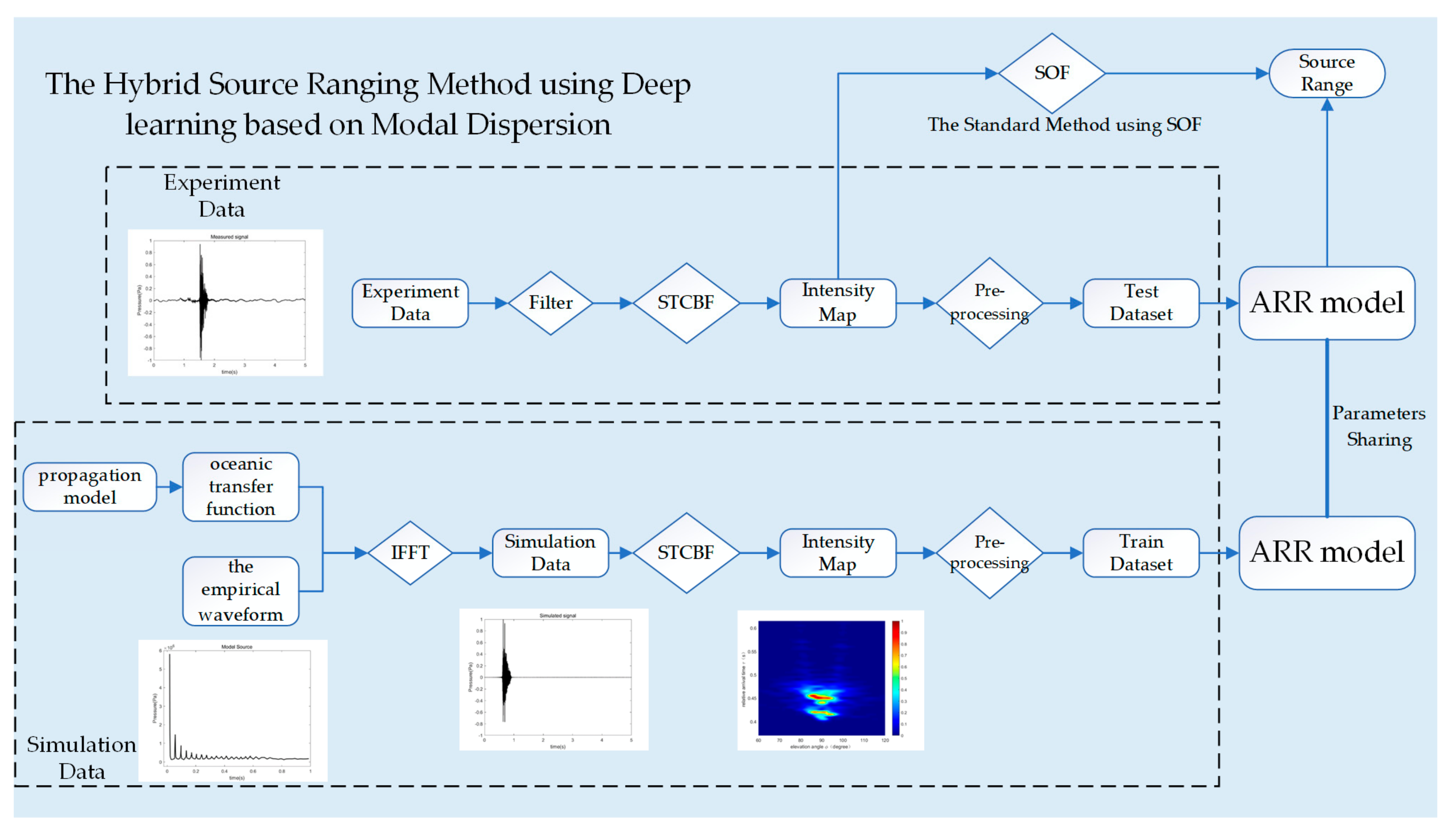
3. The Hybrid–Source Ranging Method

As previously discussed in Section 2, the standard method has limitations in its application. To overcome these limitations, we propose a Hybrid–Source ranging method, in which the intermediate results of the standard method serve as inputs for deep-learning algorithms. The flowchart presented in Figure 5 illustrates the detailed procedures for simulating the training data and processing the experimental data in the proposed method, which will be explained in the subsequent sections. Additionally, the flowchart depicts the distinctions between the standard method and the proposed method.

3.1. Input and Label

The hybrid method adopts the beam-time-domain sound-intensity map as a network input, and outputs the source range. The received signals of VLA were simulated by generating an inverse Fourier transform of the product of the oceanic-transfer function and the Fourier transform of the sound-source waveform [30]. The oceanic-transfer function was simulated using KRAKEN [31] under the environment described in Figure 6. The Kraken model is a normal-mode model developed for underwater acoustics that is robust, accurate, and efficient. It can handle a range of environmental factors, making it effective for handling sound propagation in range-independent environments. It is widely used in numerical-calculation programs based on normal-mode theory.

As shown in Figure 6, a source–receiver configuration, including a transmitting transducer and a 32-element vertical line array (VLA) with uniform element spacing of 1.5 m, is placed at a center depth of 45 m. A range-independent environment with two measured SSPs in the shallow water and a homogeneous semi-infinite basement is assumed. The detailed parameters are shown in Figure 6. A broadband time-domain pulse signal was derived from the sound source using an empirical waveform of shallow explosive charges, which is well established in [32,33], and the empirical waveform used for the simulation is shown in Figure 7. The assumed form of bubble pulses is shown in Figure 7a, and the initial pulse of bubble pulses is shown in Figure 7b.

The waveforms of the simulated signal at a range of 9.8 km and a depth of 50 m are shown in Figure 8a. Short-time CBF was performed, and the beam-time image is provided in Figure 8b.

To focus on the outline information of beam-time images and ignore unnecessary details, the output of beamforming was normalized by scaling between 0 and 1, and a specific threshold was used to preprocess the images. All points smaller than the threshold were represented by 0, and the rest remained the same.

Figure 9 shows an example of a preprocessing result with a threshold of 0.1. Before inputting the network, the dimensions of the input data were uniformly adjusted to 3 × 224 × 224. The output label is the source range. The label parameter matrix was normalized by mapping the values to [0,1]. The $i$th value, $x_i$, was transformed into $y_i$ by

$$y_i=\frac{x_i-x_{\min }}{x_{\max }-x_{\min }},i=1,2,\dots ,N,$$

(12)

where $x_{\min }$ and $x_{\max }$ denote the minimum and maximum values of the parameter matrix, respectively, and $N$ is the number of the samples.

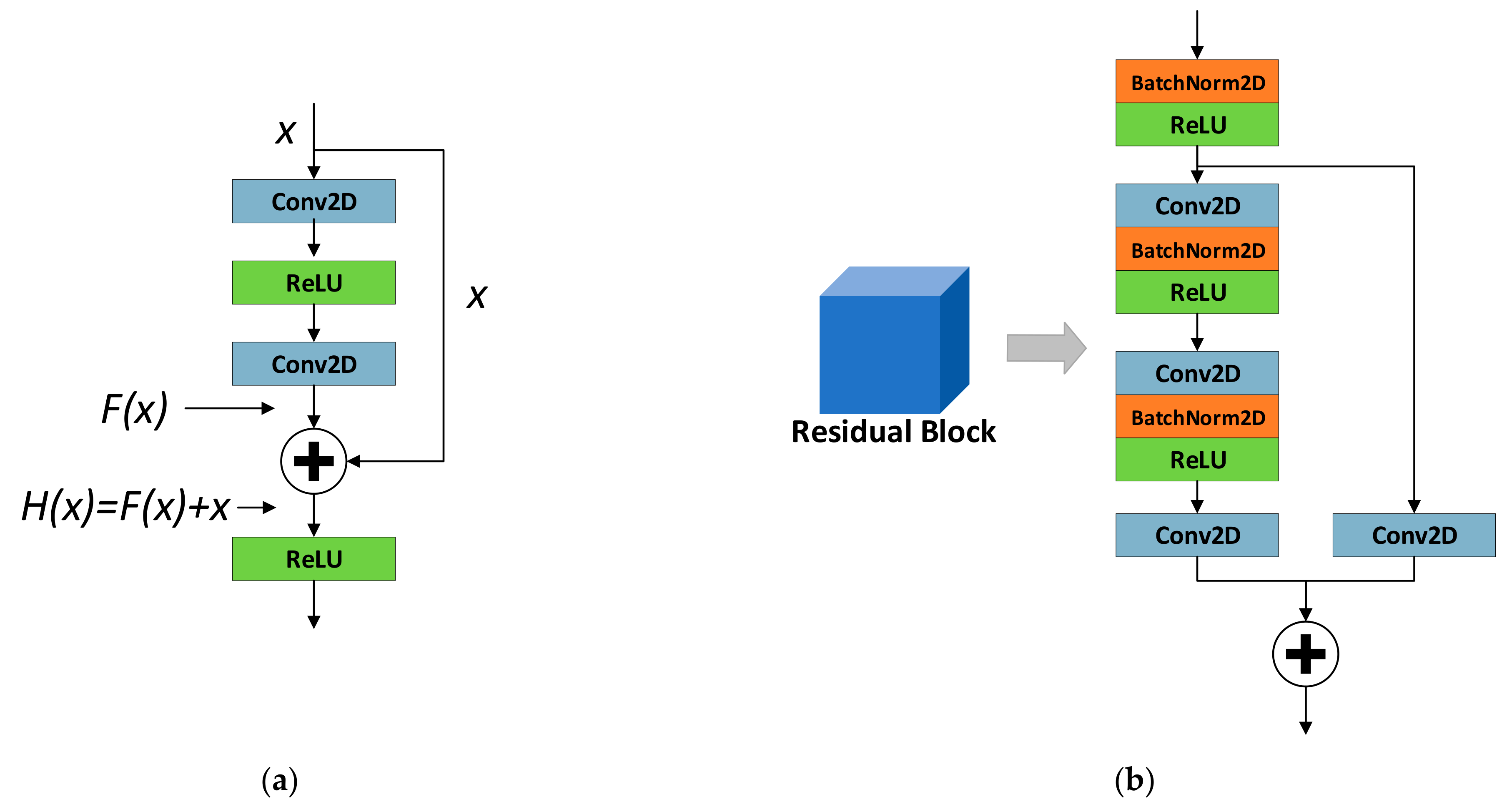
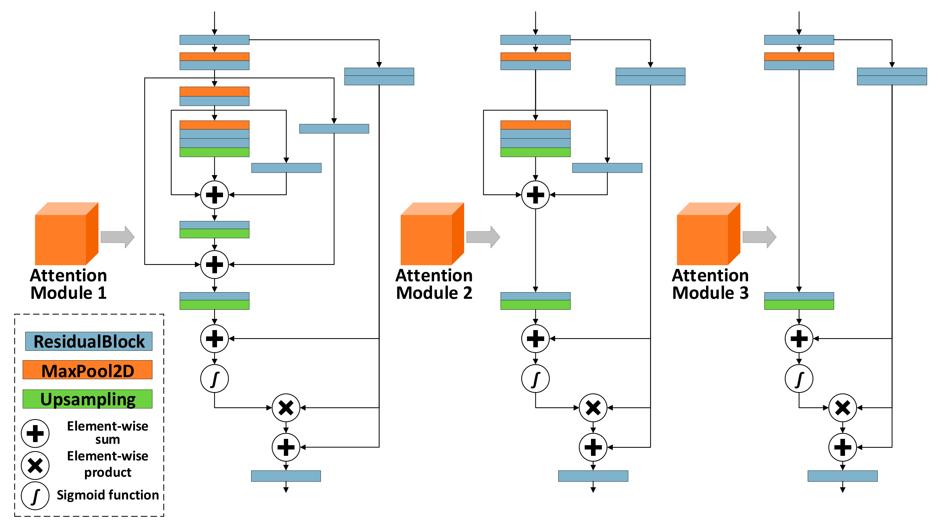
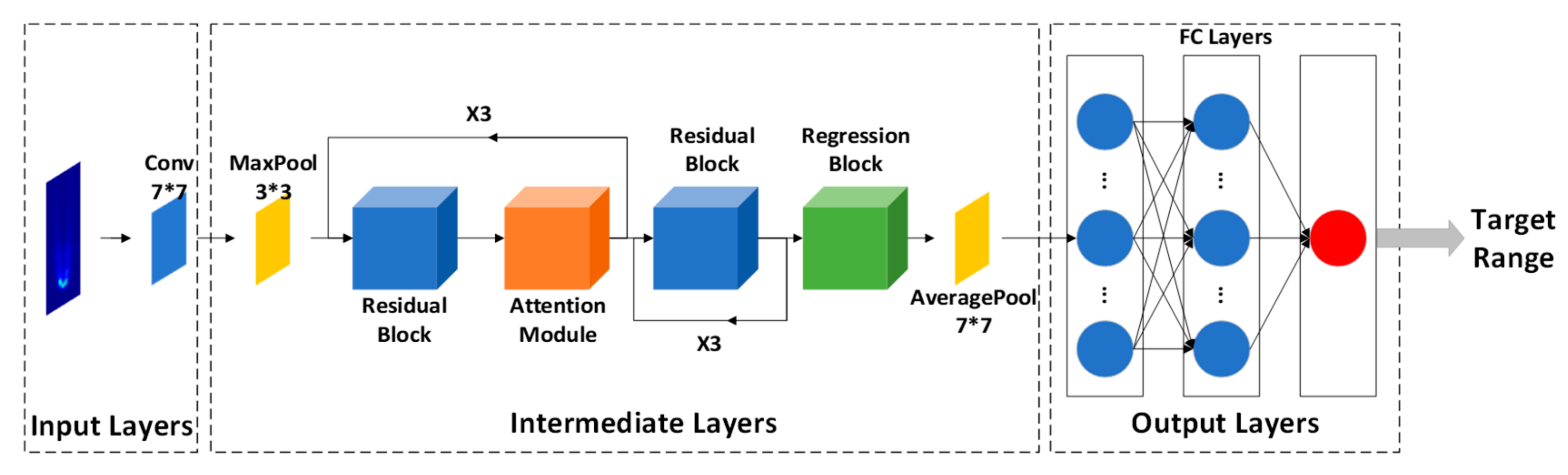
3.2. Attention-Based ResNet Regression Model(ARR)

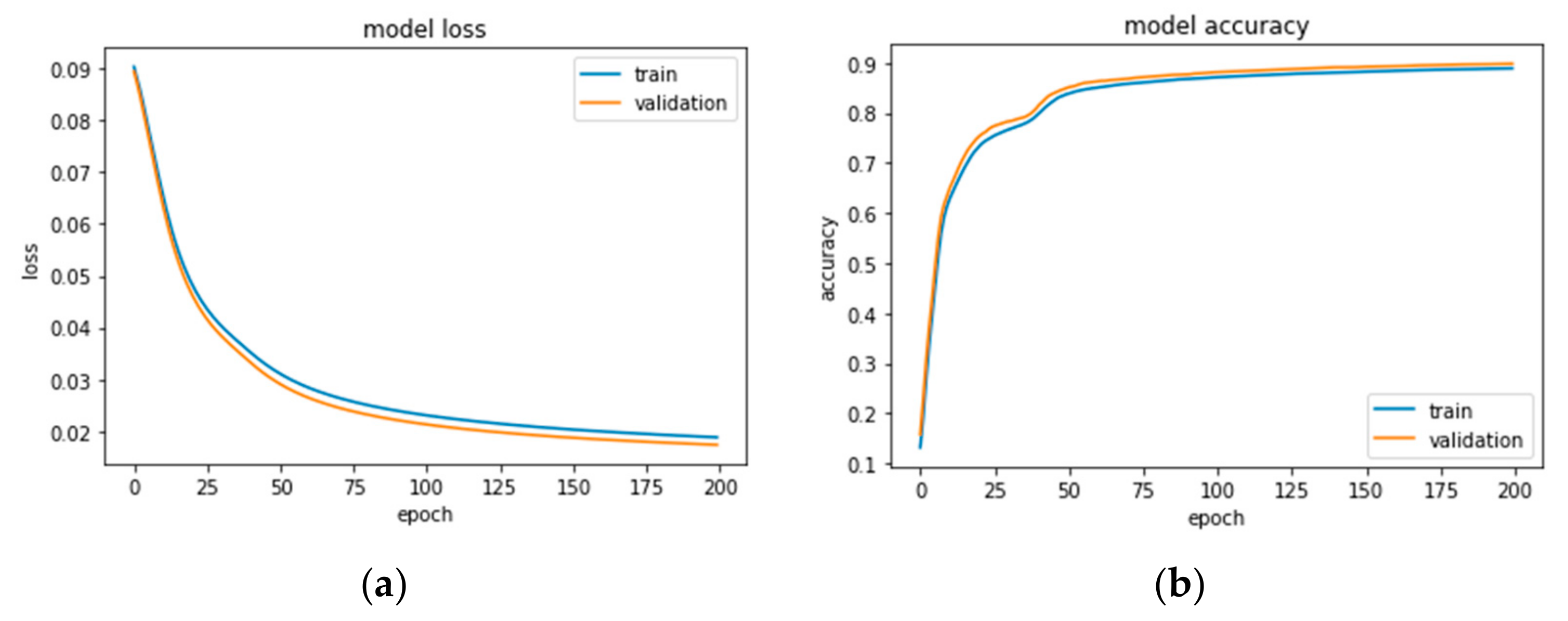
We used the residual network (ResNet) as the backbone model in the proposed model. ResNet is a new architecture, which was proposed in 2015 by researchers at Microsoft Research [28]. ResNet is one of the most powerful deep-neural networks, and achieved outstanding performance results in the ILSVRC 2015 Classification Challenge. Consequently, ResNet has been widely used as a building block in other deep-learning tasks, such as image recognition, object detection, face recognition, and image classification, thus revolutionizing the training of deep-convolutional-neural networks for computer-vision tasks.

Although many variants of ResNet architecture exist, the core idea of ResNet is the introduction of an “identity-shortcut connection” that skips one or more layers, as shown in Figure 10a [29]. With residual blocks, inputs can forward propagate faster through the residual connections across layers. Based on the core idea of ResNet, we introduced an additional convolutional layer to transform the input into the desired shape for the addition operation, and the residual block we built is shown in Figure 10b.

While the ResNet Block has more capacity, not all features contribute equally to the range regression. The attention mechanism manages to capture crucial components of a high-level semantic representation, and is typically used by natural-language processing and image processing, with various attention mechanisms. Thus, incorporating the attention mechanism can improve model performance significantly.

The principal idea behind the attention mechanism is to identify the importance of each element within a sequence of weight parameters and merge the elements according to their importance [27]. Based on the core concept of attention, the attention module collects the global information of the input and combines it with the original feature map. Additionally, a jump connection is added to capture different proportions of information at different stages. Figure 11 illustrates three basic structures of the attention module in the attention-based ResNet regression model.

Figure 12 shows the structural framework of the attention-based ResNet regression model, which is based on the residual block shown in Figure 10b and the attention module shown in Figure 11.

To quantify the prediction performance of range-estimation methods, the root-mean-square error (RMSE) over N samples is defined as

$$E_{RMSE}=\sqrt{\frac{1}{N}{\displaystyle \sum _{i=1}^N{\left({\widehat{y}}_i-y_i\right)}^2}}.$$

(13)

where ${\widehat{y}}_i$ and $y_i$ are the predicted range and the ground-truth range, respectively.

3.3. Model Training

The simulation scene settings are the same as described in Section 3.1. The parameter settings for generating the training sets are summarized in

Table 1. Parameters used for training sets.

Parameters	Units	Lower Bound	Upper Bound	No. of Discrete Values
Source depth	m	1	70	35
Source range	km	1	20	191
SSP	m/s	2 SSPs measured by CTD		2
Water depth	m	70	90	3

. We considered three seafloor topographies: two of them were range-independent shallow-sea environments, and one was the real seafloor topography shown in Figure 6. The combination of two SSPs measured by CTD, and three types of seafloor topography generated six fixed scenarios. In each scenario, 6685 (35 × 191) samples were generated under different depths and ranges. Therefore, a total of 40,110 (35 × 191 × 6) samples were obtained for the training sets.

A total of 70% of the 40,110 samples in the training set were utilized to update the weights of the learning models, while 30% of them were used for validation. The training batch size was 32, so the model was updated 590 times every epoch. The attention-based ResNet regression model used the Adam optimizer, the initial learning rate was 0.0001 with decay by a factor of 0.9 every 10 epochs, and the maximum number of iterations was 100. The network performance tended to be steady after 150 epochs, according to the training procedure shown in Figure 13. The network trained for 170 epochs was chosen for testing.

4. Experimental Demonstration

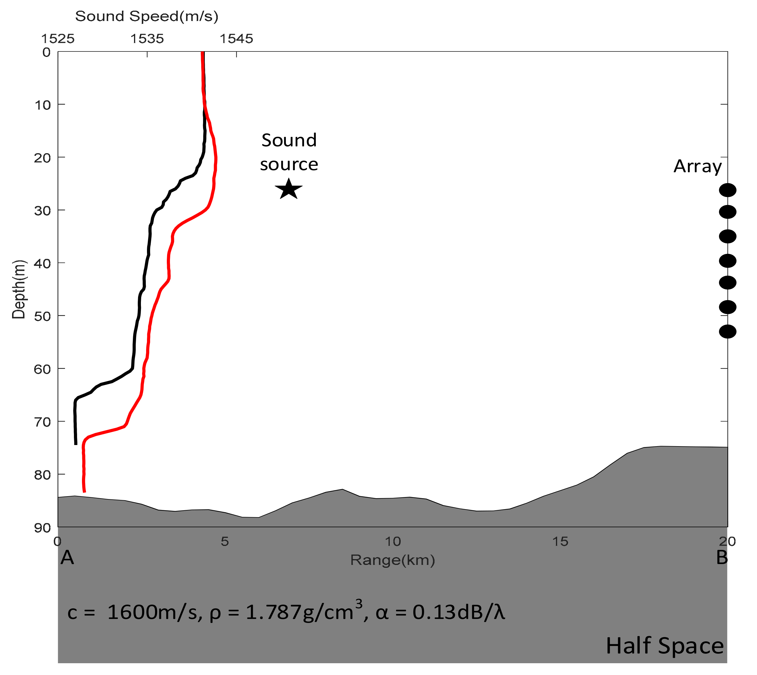
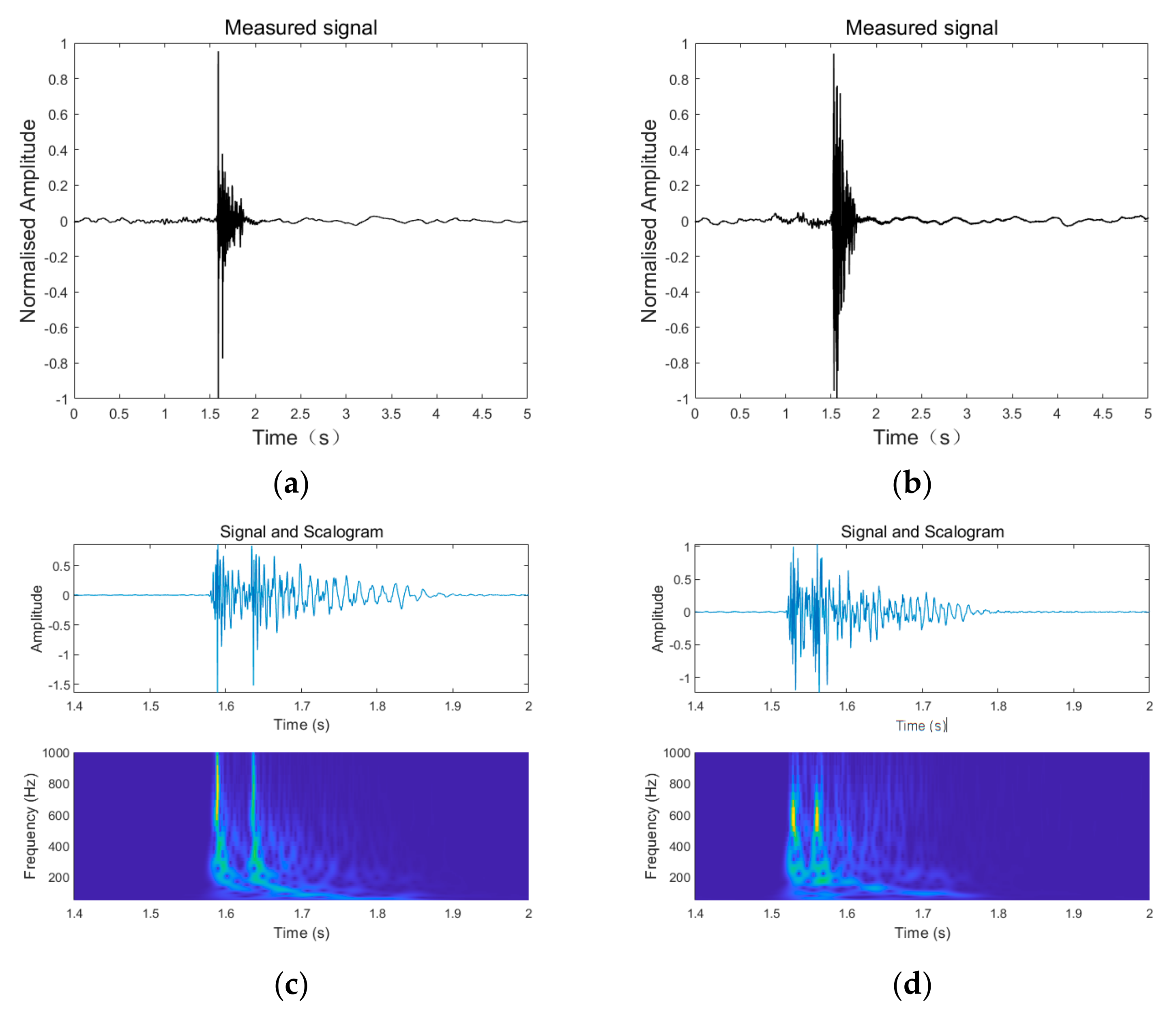
4.1. Experiment Introduction

The experimental data were obtained from the shallow-sea acoustic propagation experiment performed in July 2017. As shown in Figure 6, the receiving end at point B was a 32-element vertical line array with uniform element spacing (1.5 m), which was placed at a center depth of 45 m. Assume that a source target is at a depth of 50 m and a range of 10 km. Sound-speed profiles (SSPs) are also presented in Figure 6; SSP 1 (red) describes the SSP of the experimental sea area near point A, and SSP 2 (black) describes that near point, B. The seafloor topography shown in Figure 6 was measured during the shallow-sea acoustic-propagation experiment. A range-independent environment in the 70-m water column and a homogeneous semi-infinite basement was assumed. The ship track was from A to B. Two types of 100 g explosive sound sources were launched at different distances; one detonated at a depth of 25 m, and the other detonated at a depth of 50 m. The received signals derived from the two types of sound sources are shown in Figure 14.

Once signal processing was performed, such as filtering on the received signal, short-term CBF was performed to obtain a beam-time-domain sound-intensity image, as described in Section 2. In total, 26 intercepted signals were processed, and 26 images were generated as the test dataset of the proposed model.

4.2. Baseline Methods

To demonstrate the effectiveness of the attention-based ResNet regression model (ARR), we compared it with two baseline methods: the standard-optimization-fitting method (SOF) described in Section 2.2, and MFP. To measure the effectiveness of various methods for the ranging problem, we consider the mean relative error (MRE) and RMSE as the evaluation metrics. Specifically, assuming ${\widehat{y}}_i$ and $y_i$ are the predicted range and the ground truth range, respectively, MRE is defined as $\mathrm{MRE}=\frac{1}{N}{\displaystyle \sum _{i=1}^N\left|\frac{{\widehat{y}}_i-y_i}{y_i}\right|}$, and RMSE is denoted as $\mathrm{RMSE}=\sqrt{\frac{1}{N}{\displaystyle \sum _{i=1}^N{({\widehat{y}}_i-y_i)}^2}}$. The probability of the correct estimate was used to evaluate the accuracy of the source-range estimation, which is defined as the probability that the relative error of the range estimation is less than 10%. The proportion of reliable results in the ranging results is considered as the accuracy of the method:

$$Accuracy=\frac{{\displaystyle \sum _{i=1}^N\eta \left(i\right)}}{N}\begin{array}{cc}\times 100\%& \end{array}\left\{\begin{array}{cc}\eta \left(i\right)=1& \frac{\left|{\widehat{y}}_i-y_i\right|}{y_i}\le 0.1\\ \eta \left(i\right)=0& else\end{array}\right.$$

(14)

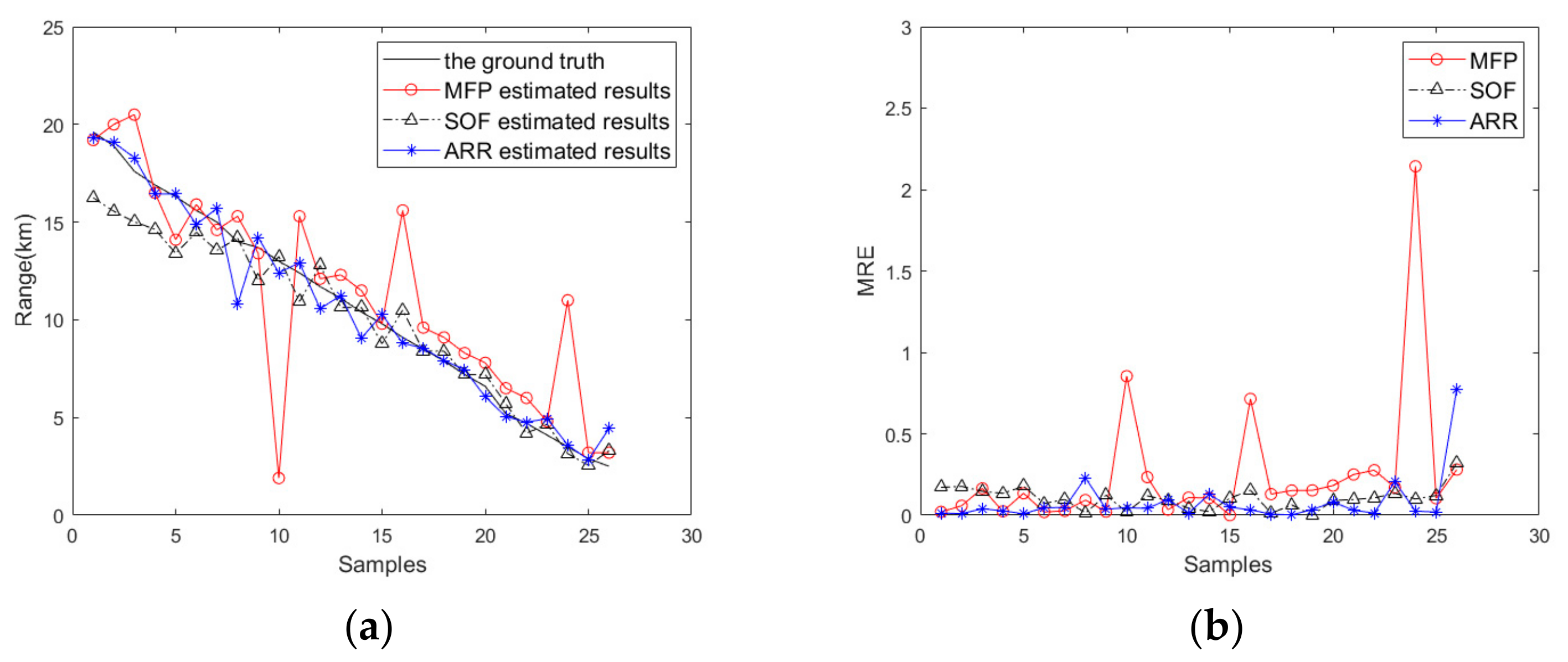
4.3. Results and Analysis

The results of different methods applied to two datasets are presented in

Table 2. Prediction performance of different models.

Models	Simulation Dataset			Experimental Dataset
	MRE	RMSE	Accuracy	MRE	RMSE	Accuracy
ARR Model	0.01	0.18	93%	0.07	0.90	85%
SOF	0.14	1.90	61%	0.18	2.54	54%
MFP	0.01	0.10	99%	0.25	3.15	35%

. These methods include the proposed Hybrid–Source ranging method based on the ARR model, the standard method utilizing the SOF approach, and the classic source-localization method, MFP. Figure 15 shows the comparison of estimated results and MREs. In general, the proposed model performed well on both simulation and experimental datasets, with the highest accuracy and lowest MRE and RMSE, verifying the effectiveness of the proposed model.

Table 2 presents a comparison of the performance of the hybrid method, the standard method, and the classical MFP method on both simulation and experimental datasets. On the simulation dataset, the hybrid method and MFP exhibit similar performances, due to the use of precise environmental parameters and propagation models to simulate the pressure field. However, on the experimental dataset, the hybrid method exhibits a significantly improved performance, with a reduction in MRE by 71% and RMSE by 2.25 km, achieving an accuracy of 85%. In contrast, the performance of MFP on the experimental dataset is lower, due to the fluctuations in shallow-sea environmental parameters and the imprecision of pressure-field simulation.

The standard method exhibits higher accuracy (54%) compared to MFP on the experimental dataset, as it uses a sound-field feature which is less affected by environmental parameters and contains source information.

In comparison, the hybrid method demonstrates a significant improvement over the standard method, reducing MRE by 66% and RMSE by 1.72 km, and improving accuracy by 57%. The poor performance of the standard method for the closest sample (No. 26) may be attributed to the insufficient range for clearly resolving the modes and mode interference. In remote distances, the standard method exhibits higher MRE compared to the hybrid method, due to differences at different ranges that are difficult to discriminate using the standard method. However, the hybrid method performs well in remote distances and achieves a lower MRE. These results demonstrate the effectiveness of the hybrid method.

5. Conclusions

In this study, a Hybrid–Source ranging method was developed using deep learning, which is based on modal dispersion in the beam-time domain to perform source ranging in shallow waters. This approach utilizes the beam-time-domain sound-intensity map, which is less affected by environmental parameters and contains source information, as input for the deep-learning network. The combination of residual network and attention mechanism was used to provide a global understanding of the images for feature extraction and evaluation, as opposed to solely relying on local features, as in conventional convolutional-neural-network approaches.

The performance of the hybrid method was compared to various baseline methods, including MFP and the standard method. The results showed that, compared to MFP, the standard method had higher accuracy (54%), due to the constant and useful features of the beam-time-domain sound-intensity map. The proposed hybrid method outperformed MFP, reducing the MRE by 71% and the RMSE by 2.25 km, and achieving an accuracy of 85%. The standard method may still be a more efficient choice in relatively simple and range-independent environments; however, the proposed method is designed to address the limitations of the standard method in distance measurement.

These results demonstrate the effectiveness and feasibility of the proposed Hybrid–Source ranging method in shallow-sea environments. The proposed method provides an effective scheme for source ranging, and has potential for practical applications.

References

1. Sazontov, A.G.; Malekhanov, A.I. Matched field signal processing in underwater sound channels (Review). Acoust. Phys. 2015, 61, 213–230. [Google Scholar] [CrossRef]
2. Baggeroer, A.B.; Kuperman, W.A.; Schmidt, H. Matched field processing: Source localization in correlated noise as an optimum parameter estimation problem. J. Acoust. Soc. Am. 1998, 83, 571. [Google Scholar] [CrossRef]
3. Jackson, D.R.; Ewart, T.E. The effect of internal waves on matched-field processing. J. Acoust. Soc. Am. 1994, 96, 2945–2955. [Google Scholar] [CrossRef]
4. Dosso, S.E.; Nielsen, P.L.; Wilmut, M.J. Data Uncertainty Estimation in Matched-Field Geoacoustic Inversion. J. Acoust. Soc. Am. 2006, 119, 208–219. [Google Scholar] [CrossRef]
5. Wilcox, P.D.; Lowe, M.; Cawley, P. A signal processing technique to remove the effect of dispersion from guided wave signals. Aip Conf. Proc. 2001, 557, 555–562. [Google Scholar]
6. Chuprov, S.D. Interference structure of a sound field in a layered ocean. In Ocean Acoustics. Current State; Brekhovskikh, L.M., Andreevoi, I.B., Eds.; Nauka: Moscow, Russia, 1982; pp. 71–91. [Google Scholar]
7. Turgut, A.; Orr, M.; Rouseff, D. Broadband source localization using horizontal-beam acoustic intensity striations. J. Acoust. Soc. Am. 2010, 127, 73. [Google Scholar] [CrossRef]
8. Yun, Y.; Junying, H. Passive ranging based on acoustic field interference structure using double arrays(elements). Chin. J. Acoust. 2012, 31, 262–274. [Google Scholar] [CrossRef]
9. Yang, T.C. Beam intensity striations and applications. J. Acoust. Soc. Am. 2003, 113, 1342–1352. [Google Scholar] [CrossRef]
10. Wang, N. Dispersionless transform and potential application in ocean acoustics. In Proceedings of the 10th Western Pacific Acoustics Conference, Beijing, China, 21 September 2009. [Google Scholar]
11. Gao, D.; Wang, N. Dispersionless transform and signal enhencement application. In Proceedings of the 2th International Conference on Shallow Water Acoustic, Shanghai, China, 13 April 2009. [Google Scholar]
12. Gao, D.; Wang, N.; Wang, H. Artifical time reversal mirror by dedispersion transform in shallow water. In Proceedings of the 3th Oceanic Acoustics Conference, Beijing, China, 12 May 2012. [Google Scholar]
13. Gao, D. Waveguide Invariant in Shallow Water: Theory and Application. Ph.D. Thesis, Ocean University of China, Qingdao, China, 2012. [Google Scholar]
14. Xiao-Le, G.; Kun-De, Y.; Yuan-Liang, M.; Qiu-Long, Y. A source range and depth estimation method based on modal dedispersion transform. Acta Phys. Sin. 2016, 65, 214302. [Google Scholar] [CrossRef]
15. Zhang, S.; Zhang, Y.; Gao, S. Passive acoustic location with de-dispersive transform. In Proceedings of the 16th Western China Acoustics Conference, Leshan, Sichuan, China, 1 August 2016. [Google Scholar]
16. Lee, S.; Makris, N.C. The array invariant. J. Acoust. Soc. Am. 2006, 119, 336–351. [Google Scholar] [CrossRef]
17. Lee, S.; Makris, N.C. A new invariant method for instantaneous source range estimation in an ocean waveguide from passive beam-time intensity data. J. Acoust. Soc. Am. 2004, 116, 2646. [Google Scholar] [CrossRef]
18. Lee, S. Efficient Localization in a Dispersive Waveguide: Applications in Terrestrial Continental Shelves and on Europa. Ph.D. Thesis, Massachusetts Institute of Technology, Cambridge, MA, USA, 2006. [Google Scholar]
19. Kong, Q.; Trugman, D.; Ross, Z.; Bianco, M.; Meade, B.; Gerstoft, P. Machine learning in seismology: Turning data into insights. Seismol. Res. Lett. 2018, 90, 3–14. [Google Scholar] [CrossRef] [Green Version]
20. Bergen, K.J.; Johnson, P.A.; de Hoop, M.V.; Beroza, G.C. Machine learning for data-driven discovery in solid earth geo-science. Science 2019, 363, eaau0323. [Google Scholar] [CrossRef]
21. Zhenglin, L.I.; Haibin, W.A.N.G. Overview of Machine Learning Methods in Underwater Source Localization. J. Signal Process. 2019, 35, 1450–1459. [Google Scholar]
22. Liang, X.; Yang, F. Underwater Acoustic Target Localization: A Review. IEEE J. Ocean. Eng. 2021, 46, 112–125. [Google Scholar] [CrossRef]
23. Soylu, C.; Basyigit, B.; Tekin, A.C. Machine Learning Methods for Underwater Acoustic Localization: A Survey. IEEE Access 2020, 8, 130589–130611. [Google Scholar] [CrossRef]
24. Li, L.; Chen, H. Underwater Acoustic Target Localization: A Review of Recent Progress and Challenges. Sensors 2020, 20, 6599. [Google Scholar] [CrossRef]
25. Torres, D.; Casari, P.; Zuniga, M. A Review of Machine Learning Techniques for Acoustic Target Localization in Underwater Sensor Networks. Ad Hoc Netw. 2018, 73, 65–79. [Google Scholar] [CrossRef]
26. Niu, H.; Ozanich, E.; Gerstoft, P. Ship localization in Santa Barbara Channel using machine learning classifiers. J. Acoust. Soc. Am. 2017, 142, EL455–EL460. [Google Scholar] [CrossRef] [Green Version]
27. He, K.; Zhang, X.; Ren, S.; Sun, J. Deep residual learning for image recognition. In Proceedings of the IEEE Conference on Computer Vision and Pattern Recognition, Las Vegas, NV, USA, 26 June–1 July 2016; pp. 770–778. [Google Scholar]
28. Wang, F.; Jiang, M.; Qian, C. Residual attention network for image classification. In Proceedings of the 2017 IEEE Conference on Computer Vision and Pattern Recognition (CVPR), Honolulu, HI, USA, 21 July 2017; pp. 3156–3164. [Google Scholar]
29. Vaswani, A.; Shazeer, N.; Parmar, N.; Uszkoreit, J.; Jones, L.; Gomez, A.N.; Kaiser, Ł.; Polosukhin, I. Attention is all you need. arXiv 2017, arXiv:abs/1706.03762. [Google Scholar]
30. Jensen, F. Computational Ocean Acoustics, 2nd ed.; Springer Science Business Media, LLC.: New York, NY, USA, 2011; pp. 611–617. [Google Scholar]
31. Porter, M.B. “The KRAKEN Normal Mode Program”, SACLANT Undersea Research Centre Memorandum SM-245 and Naval Research Laboratory Memorandum Report No. 6920. 1991. Available online: http://oalib.hlsresearch.com/Modes/kraken.pdf (accessed on 1 March 2023).
32. Chapman, N.R. Measurement of the waveform parameters of shallow explosive charges. J. Acoust. Soc. Am. 1985, 78, 672–681. [Google Scholar] [CrossRef]
33. Gannon, L. Simulation of underwater explosions in close-proximity to a submerged cylinder and a free-surface or rigid boundary. J. Fluids Struct. 2019, 87, 189–205. [Google Scholar] [CrossRef]
Figure 1. Measured signals received by VLA at (a) 2.9 km and (b) 19.6 km, which indicates the waveform expansion.
Jmse 11 00561 g001
Figure 2. Measured signal received by VLA at 9.8 km.
Jmse 11 00561 g002
Figure 3. (a) The sound-intensity map in beam-time domain generated by performing STCBF on measured signal; (b) t ~ 1 / sin ( ϕ ) relationship obtained by SOF.
Jmse 11 00561 g003
Figure 4. Simulated sound-intensity maps at (a) 18 km and (b) 20 km.
Jmse 11 00561 g004
Figure 5. The scheme of the Hybrid–Source Ranging Method.
Jmse 11 00561 g005
Figure 6. Waveguide parameters and source-receiver configuration using for simulation.
Jmse 11 00561 g006
Figure 7. (a) Empirical waveform, (b) initial pulse.
Jmse 11 00561 g007
Figure 8. (a) Simulated signal and (b) beam-time images generated on it.
Jmse 11 00561 g008
Figure 9. Preprocessing result with a threshold of 0.1; (a) original beam-time image, (b) preprocessed-input image.
Jmse 11 00561 g009
Figure 10. (a) Typical structure of the residual block, (b) residual block with additional convolution.
Jmse 11 00561 g010
Figure 11. Structures of attention modules 1, 2, 3.
Jmse 11 00561 g011
Figure 12. Algorithm flowchart using the attention-based ResNet regression model.
Jmse 11 00561 g012
Figure 13. Training process of the network, (a) loss, (b) accuracy.
Jmse 11 00561 g013
Figure 14. Received signals derived from explosive-sound sources, which detonated at (a) 25 m and (b) 50 m, (c,d) filtered signals in the time domain and their wavelet scalograms.
Jmse 11 00561 g014
Figure 15. (a) Estimated results and (b) MRE of MFP, SOF and ARR on the test set.
Jmse 11 00561 g015