Abstract
A simple CFD-based data-driven reduced order modeling method was proposed for the study of damaged ship motion in waves. It consists of low-order modeling of the whole concerned parameter range and high-order modeling for selected key scenarios identified with the help of low-order results. The difference between the low and high-order results for the whole parameter range, where the main trend of the physics behind the problem is expected to be captured, is then modeled by some commonly used machine learning or data regression methods based on the data from key scenarios which is chosen as Piecewise Cubic Hermite Interpolating Polynomial (PCHIP) in this study. The final prediction is obtained by adding the results from the low-order model and the difference. The low and high-order modeling were conducted through computational fluid dynamics (CFD) simulations with coarse and refined meshes. Taking the roll Response Amplitude Operator (RAO) of a DTMB-5415 ship model with a damaged cabin as an example, the proposed physics-informed data-driven model was shown to have the same level of accuracy as pure high-order modeling, whilst the computational time can be reduced by 22~55% for the studied cases. This simple reduced order modeling approach is also expected to be applicable to other ship hydrodynamic problems.
1. Introduction
When a ship encounters accidents such as collision and grounding during navigation, damage to the ship might cause flooding to the cabin which will threaten the safety of the ship. More specifically, through the damaged part of the ship hull, water will quickly rush into the cabin and then dramatically change the weight and buoyancy distribution. The ship will then experience large motion and additional load due to this flooding. Excessive flooding can eventually cause the ship to sink or capsize. Typical examples include the accidents of the vessels ‘Costa Concordia’, ‘Herald of free enterprise’, ‘Estonia’ and the sinking of the ‘Sewol’ South Korea [1,2,3,4]. From van den Boom’s [1] analysis of the ‘Sewol’, it can be seen that flooding will have a great impact on a ship. For naval ships or ships away from the shore, the damaged ships often have to continue navigation until reaching the nearest port or safe place. Therefore, the seakeeping performance of a damaged ship in waves is a vital part for evaluating the ship’s survivability, especially for naval ships. Accurate and practical tools for evaluating the flow and motion of the damaged ship is important for both academics and designers of ships.
The research into the motions of damaged ships has been conducted by theoretical, experimental and numerical methods. In terms of theoretical research, some typical examples include that Lee [5] established a time-domain theoretical model to predict damaged ship motion and flooding for any ship type or arrangement; Xu [6] established the mathematical model of instantaneous water inflow velocity and volume of the damaged cabin based on the basic principle of hydrodynamics, and analyzed the effects of parameters such as loading conditions; Zhang [7] solved the floating equilibrium equation of a damaged ship in a time-domain by means of a quasi-static method.
In terms of experimental research, Lee [8] conducted free roll free decay experiments on intact and damaged ships in still water and regular waves conditions, and analyzed the influence of flooding on ship roll decay motion; Begovic [9] conducted experiments on models with different scales for intact and damaged DTMB-5415 ships in different wave conditions, and the effects of damage positions on a ship’s RAO; Domeh [10] studied the influence of the permeability, arrangement and orifice size of the cabin on a ship’s motion characteristics in waves; Maria Acanfora [11,12] conducted experimental research on passenger ships, mainly about the influence of the damage location, opening size and moving objects in the engine room on the motion characteristics of damaged ships in still water and regular waves.
Compared with experiments, numerical methods are relatively low-cost and can conveniently reproduce the physics behind the process as much as possible. As a consequence, various numerical methods have been successfully applied to many hydrodynamic problems and the research on damaged ships is no exception. Some representative works are reviewed as follows: Bašić [13] presented the prediction of the total resistance of an intact and damaged ship model using the CFD technique. Chan [14] proposed a nonlinear time-domain simulation method to predict the wave load of intact and damaged RO-RO ships in regular wave conditions; Gao conducted a series of work for the problem of damaged ship flow by CFD methods [15,16] including developing a finite volume-type Navier–Stokes solver based on volume of fluid (VOF) and dynamic meshing techniques, and the systematic CFD investigations [17] for the effect of air compressibility, damaged cabin arrangement and encountered wave height on the damaged ship motion and flooding process. Furthermore, Gao [18] improved computational efficiency by combing the potential flow theory for global seakeeping solving and the Navier–Stokes solver for a local cabin flooding simulation; the mesh-less-type CFD methods were also used for damaged ship flow investigations such as the work of Ming [19] by smoothed particle hydrodynamics (SPH) and Zhang’s [20] work by the moving particle semi-implicit (MPS) method.
Generally, the complexity of the flooding flow for damaged ships often involves violent free surface breaking, high viscosity effects, etc.; hence, the more time-consuming CFD method instead of potential flow theory must be used to accurately capture the physics of the flow as discussed above. However, the CFD computation efficiency can be a problem for large-scale simulations such as the systematic simulation for effects by various parameters, even with the rapidly developed computational power. Some kind of model order reduction would be desirable, under the requirement that the dominant physical process has to be included in the reduced order model. Various ideas have been proposed for such purpose. For example, Xiao [21] developed a novel Non-Intrusive Reduced Order Model (NIROM) for the fluid–structure interaction (FSI) based on proper orthogonal decomposition (POD) and the radial basis function (RBF) interpolation method. This model was applied to three coupling simulations; the calculation time is greatly reduced while high-fidelity details were captured; Whisenant [22] combined POD and a neural network framework for the purpose of reconstructing and predicting both the fluid and structural fields of the Turek–Hron FSI benchmark problem in order to minimize computational effort and time. Sufyan [23] applied the POD analysis on the pressure field data obtained from numerical simulations of the flow past stationary and oscillating cylinders and proposed the development of a more effective reduced-order model based on this research. Apart from these POD-type flow modal decomposition approaches, pure data-driven machine learning techniques have also been applied to capture the main features of complex flow such as the work of Wu [24], where a convolutional neural network (CNN) was used to conduct the flow modal decomposition and then reconstruct the flow by the extracted low-order modes. All of the above authors have conducted pioneering work, but their methods are complex and difficult to replicate. In this paper, an even simpler yet effective data-driven approach was proposed for reducing the modeling order of complex damaged ship flows in waves, where the main flow feature identification was simply conducted by a low resolution CFD simulation.
2. Methodology
2.1. Data-Driven Reduced Order Modeling
The data-driven models have been successfully applied in many fields [25,26,27]. Normally, a pure data-driven model will act as a “black-box”, where the physics behind the concerned problem is not required to be known as a priori. Although this model requires a sufficient amount of high-quality data, this is an important advantage for many complicated physical processes, especially the problems arising from industrial practice (damaged ship motion is one of them). More specifically, the input parameters and the system responses can usually be readily obtained by either an experimental measurement or high-fidelity simulation, but the physics behind this process could be too complicated to be explicitly described by a compact function. The general idea of data-driven models is that for a given set of data , the unknown function between input and output , that is , can be approximated as , i.e.,
The specific form of can be obtained via various machine learning/data regression models, e.g., artificial neural network (ANN) [28,29,30], deep learning (DL) [31], singular value decomposition (SVD) [32] and support vector machine (SVM) [33]. In this paper, a simple and commonly used data regression model called Piecewise Cubic Hermite Interpolating Polynomial (PCHIP) is adopted. In a PCHIP interpolation, the form of is chosen in the following way:
where , n is the total number of elements for ( is of the same size as ) and is a series of cubic polynomials that collectively guarantee that the first and second order derivatives are continuous at each input parameter . The fitting of the data will use the PCHIP method in the MATLAB Curve Fitting toolbox. The data interpolation was conducted in MATLAB and more implementation details can be found in Ref. [34]. The approximated relation between and , i.e., , can then be used to describe and predict the system response for other input parameters that are within the range of interpolation for the training data set, i.e., .
Although such models have been proven to be effective for a large variety of problems [35,36], the accuracy is largely dependent on the amount and quality of the training data. This means a large set of scenarios of the investigated problem has to be either simulated by high-fidelity, first-principle-based methods, such as CFD or computational structure dynamics (CSD), or measured by carefully designed experiments. Therefore, these kind of pure data-driven approaches cannot be very cost effective.
In this paper, the pure data-driven modeling approach is enhanced by the first-principle-based model i.e., CFD, so the main characteristics of the physics behind the problem can be implicitly embedded in the model. More specifically, similar to the ideas of [37,38,39,40], a low-order model is first used to capture the system response for the whole range of parameters . Although the precision of is low, the general pattern of the physics behind this process can still be revealed to some extent. Therefore, with the help from the low-order model, the input parameters correspond to the key scenarios, such as the peaks, and turning points can be identified, i.e., is a subset of . After that, the more time-consuming high-order model can be used to re-calculate the limited number of system responses corresponding to .
Next, as a key step of the proposed model, the pattern of the difference between low- and high-order model predictions for input data is then modeled by some data regression model. That is, if the sub-set of the low-order prediction data corresponding to is denoted as , i.e., , the machine learning or data regression methods are applied to approximate the relation between and the difference , i.e.,
As a result, the difference between low- and high-order models for the whole range of input variables can be readily interpolated from the approximated function as
Finally, the system response for the whole parameter range can be approximated as the addition of and :
If the system response prediction for the whole parameter range by a pure high-order model is denoted as , it is expected that has the same level of accuracy as , since we assume that the main physics can be captured by the data from low-order model (which is proven to be reasonable as shown in the discussion of Section 3). In the meanwhile, the computation time for the proposed model, i.e., the low-order model computation for the whole parameter range and high-order model for a limited number of key scenarios, can be considerably lower compared to the approach using a pure high-order model for the whole parameter range. This will be discussed in detail later in Section 3. It is worth emphasizing that the convenience of a pure data-driven model is still kept in this approach, i.e., only low and high-order simulation data are needed and the explicit expression of the physics behind the concerned system is not required as a priori. Figure 1 shows the main flow of our proposed model.
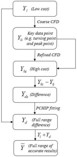
Figure 1.
Workflow of the proposed model.
The low- and high-order models can be chosen from various commonly used first-principle-based models. In this paper they are chosen to be CFD simulations with coarse and refined meshes, which will be called coarse and refined CFD, respectively. The details of the CFD model will be provided in the next section.
2.2. First-Principle-Based Model-CFD
2.2.1. CFD Model and Ship Geometry
The CFD simulation was conducted using the commercial software STAR-CCM+, where the Reynolds Averaged Navier–Stokes (RANS) equation is solved. The turbulence of the flow was modeled through SST K-Epsilon and the VOF model was used for the free surface modeling. A Eulerian multi-phase flow solver was chosen for the computation. The Semi-Implicit Method for Pressure Linked Equations (SIMPLE) algorithm was used for coupling the pressure and velocity field. We have used second-order convection and first-order time-discrete formats. More details of the software implementation can be found in Ref. [41].
The ship model used in this study is DTMB-5415, which is shown in Figure 2. The details of the geometry are listed in Table 1. The size and location information of the damaged cabin were obtained from the experiment of Begovic [42], which can be seen from Figure 2 as well.
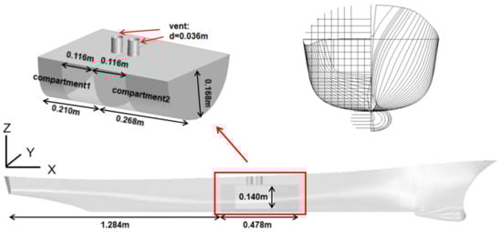
Figure 2.
Geometry of the ship model.

Table 1.
The main geometry parameters of the DTMB-5415 ship.
The roll motion under beam sea conditions was investigated and the wave conditions, which includes wave periods , wave length , and wave height , used in the computation are listed in Table 2.
Table 2.
The wave conditions used in the computation.
The mesh and boundary conditions of the computational domain is shown in Figure 3 and Figure 4. The grid base size is 0.024 m and the grid has been refined for areas with a complex flow or geometry, including free surfaces and hull boundaries. The use of overlapping meshing techniques allows for a better simulation of the hull’s movements. Pressure outlet and wall boundary conditions were enforced on the top and bottom of the computational domain, respectively, whilst the velocity inlet conditions were imposed on the four sides of the computational domain. Wave damping was imposed around the four sides of the computational domain as well.
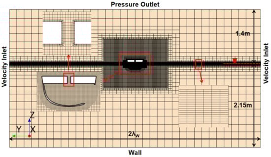
Figure 3.
Mesh and boundary conditions (front view).
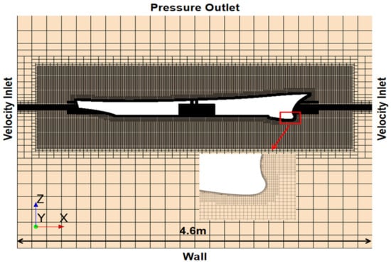
Figure 4.
Mesh and boundary conditions (side view).
2.2.2. Model Validation
The mesh and time step dependencies of the CFD model were first checked through the wave propagation problem [43]. We used fifth order Stokes waves as a wave model. For the mesh size, within the scope of one wave height, the free surface area was discretized by 8, 12, and 16 layers, respectively. For the time step, the values of 0.001 s, 0.002 s, and 0.004 s were chosen for the checking. The performances are shown in Figure 5 and Figure 6. It can be seen that the results with 12- and 16-layer meshes around the free surface are very close and both of them match with the theoretical prediction very well. Similarly, the results with time steps of 0.001 s and 0.002 s also show better accuracy. Therefore, the 12-layer free surface meshing strategy and the time step of 0.002 s were finally chosen for the following computation as a result of the trade-off between efficiency and accuracy. Figure 7 shows the free liquid surface calculation cloud for a wave height of 0.118 m and a wave period of 1.47 s.
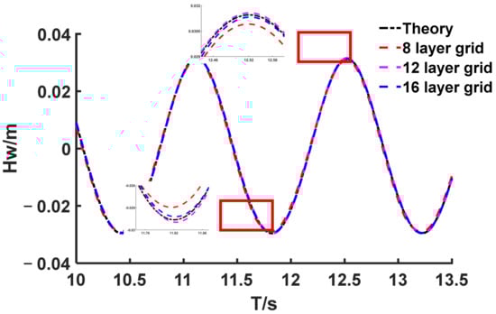
Figure 5.
Time histories of wave elevations obtained by the numerical simulation and theory (Tw = 1.4 s).
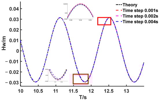
Figure 6.
Time histories of wave elevations obtained by the numerical simulation and theory (Tw = 1.4 s).
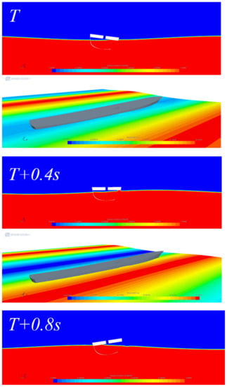
Figure 7.
Plot at the free surface with a wave period of 1.47 s and a wave height of 0.118 m.
In the calculations, we used the wall function and to ensure the accuracy of the calculations the y+ value of the hull surface always does not exceed 50. Figure 8 shows the y+ values on the hull surface. The accuracy of the whole computation model was validated against Begovic’s [42] experimental result of the roll RAO of the DTMB-5415 model with a damaged cabin (Figure 2). The roll angle of the ship is dimensionless and was scaled with by the wave number K = /λw and wave amplitude A = Hw/2 and shown in Figure 9.
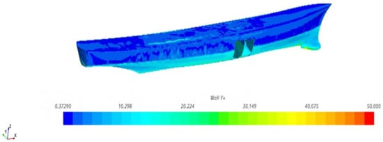
Figure 8.
Y + values on the hull surface.
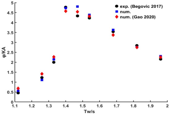
Figure 9.
Comparison of the pure refined CFD and reference results [18,42].
The numerical results by the adopted model are generally in good agreement with the experiments. Table 3 shows the comparison between refined CFD and the experimental data. The average error compared with experimental results is 8%. The results obtained from the adopted CFD model also show generally better performance than the simulation results reported by Gao [18]. However, the numerically predicted response for the wave period of 1.47 s is higher than the experimental value. The numerical result of Gao [18] also shows an overestimation at this wave period. This could be caused by the slight deviation of the shape of the cabin, which is not clearly provided in the paper of Begovic [42]. This shape difference may have a greater influence around resonances. Nevertheless, the main purpose of this paper is to show the data-driven model enhanced by the combination of high- and low-order simulation results can be as reliable as the time-consuming prediction by a pure high-order simulation.
Table 3.
The wave conditions used in the computation.
3. Results and Discussion
3.1. The Accuracy of the Proposed Model
The accuracy of the predictions was measured by the mean absolute error (MAE) as defined in Equation (6):
where n is the number of the cases (i.e., the incident waves periods) used for the comparison, i.e., the number of testing points; is the predicted system responses; and means the reference values, which are chosen as the experimental results by Begovic [42].
As stated in Section 2.1, the proposed model includes a coarse CFD simulation on the whole parameter range and a refined CFD simulation for some limited parameters. The performance of the proposed model with different choices of the high-order model data is an important factor that affects the robustness of the method. In sections 4, 5, and 6, incident wave periods among a total of nine periods were simulated by refined CFD (which will be called training data). Correspondingly, the data of 5, 4, and 3 incident wave periods were then left for checking the performance of the proposed models (which will be called testing data). For each number of wave periods, eight different ways of choosing the specific periods were investigated. The general principle of incident wave periods selection is that the first and last one within the whole range were always included, then at least one period close to the RAO peak was also chosen. Apart from that, the periods were chosen randomly. This is because if the values at key parameters are missing, the pattern revealed by the low-order model (rough CFD) will certainly be expected to be problematic, whilst it would be desirable that the position of other data should not have a significant effect on the overall performance. The details of incident wave periods selection are listed in Table 4, Table 5 and Table 6.
Table 4.
Arrangement of training and testing data (6 training data points).
Table 5.
Arrangement of training and testing data (5 training data points).
Table 6.
Arrangement of training and testing data (4 training data points).
For the refined and coarse CFD simulation, the mesh number used for each incident wave period is shown in Table 7. It can be seen that the mesh numbers are significantly less for the coarse CFD simulations. It also should be mentioned that the time steps for the wave periods of 1.40 s and 1.47 s were chosen to be 0.015 s instead of 0.02 s for the rest of the cases, since the results were more sensitive to the choice of time step around resonance.
Table 7.
Mesh numbers for different cases.
In order to illustrate the detailed implementation steps of the proposed model, the case no. 2 in Table 4 will be taken as an example for detailed discussion and the results are shown in Figure 10. The black line represents the final result obtained through the model, the red line represents the result of the coarse CFD simulation, the pink line represents the difference result between the refined and coarse CFD simulations, the blue dotted line represents the result obtained by direct fitting of the training data (black star), the black star represents the result of the refined CFD simulation corresponding to the training wave period, the red star represents the result of the refined CFD simulation corresponding to the verification wave period, and the red dot represents the experimental data. In this case, the responses for six incident wave periods were selected as the training data. The coarse CFD simulation on all nine incident wave periods was first conducted as marked by the red dot-line. The difference between the refined and coarse CFD simulation on the positions of the training data (black star) were then interpolated by PCHIP as marked by the pink dot-line. After that, the responses (black line) for the whole range of wave periods can be obtained by adding the coarse CFD results (red line) and the interpolated difference (pink line).
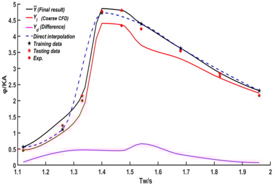
Figure 10.
The performance of the proposed model for case no. 2 in Table 3.
As shown in Figure 10, the approximation by the proposed model (i.e., the black line) is very close to the direct refined CFD simulation results (black and red stars), especially at the testing data points (red stars). The MAE for the refined CFD results and the results by the proposed model are 0.1525 and 0.1552, respectively, which shows that the proposed model has the same level of accuracy as the refined CFD.
On the other hand, if we directly use the training data to approximate the response on the whole wave period range (also by PCHIP), the results can be problematic. As shown by the blue line in Figure 10, this approximation considerably deviates from the refined CFD results, especially at the wave periods of 1.33 s and 1.47 s (testing points). The MAE for the direct PCHIP interpolation approximation by the training data is 0.2319, which is about 1.5 times the error by the proposed model.
Moreover, the direct interpolation by the training data shows a very strong dependency on the way of data selection, which can be clearly shown by comparing the blue lines in Figure 10 and Figure 11. More specifically, although for both cases the first, last, and one point around the peaks of the refined CFD results were all included in the training data set, the position of the interpolation peaks and the curve trend were very different, whilst the proposed model shows very consistent prediction results for these two sets of training data as shown by black lines in Figure 10 and Figure 11. In terms of error, the MAE for the proposed model is only 0.16 (in the same level of the results in Figure 10), whilst the MAE for direct interpolation by the training data is 0.2775, which is about 1.7 times the error by the proposed model.
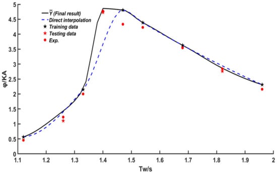
Figure 11.
The performance of the proposed model for case no. 4 in Table 4.
The MAEs for all 24 sets of training data by the proposed model, direct interpolation by the training data, and the pure refined CFD for the whole parameter range are shown in Figure 12. It can be seen that the proposed method gives the same level of accuracy as the pure refined CFD method for all the 24 sets of training data and more data included in the training data set will generally improve the performance. More specifically, for the proposed model, the mean value of MAEs by using 4, 5, and 6 wave periods training data are 0.1814, 0.1586, and 0.1604, whilst the MAE of the pure refined CFD is 0.1524. The accuracies are generally considerably lower than the proposed model results for the same training data set, i.e., the corresponding MAEs for direct interpolation from the training data are 0.6157, 0.2934, and 0.2171.
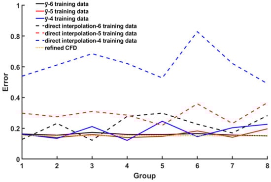
Figure 12.
The MAE for the proposed method and direct PCHIP interpolation by different training data sets (i.e., 4, 5, and 6 wave periods) and pure refined CFD (i.e., 9 wave periods).
For the data dependency, the proposed model is minor as well, especially for cases with more training data. On the contrary, the direct interpolation by the training data shows a strong variation for different data sets and data numbers. The standard deviation (SD) can be a good measure of data variation, which is used for evaluating the level of data dependency of the proposed model. For each number of training data, i.e., 4, 5, and 6, the SDs for the eight different ways of selecting data were calculated. The results for the proposed model with the 4, 5, and 6 training data are 0.0066, 0.0199, and 0.0434, whilst the direct interpolation of the training data give 0.0654, 0.0497, and 0.0998.
3.2. Efficiency of the Proposed Model
The computational efficiency of the proposed model is discussed in this part. Since the data interpolation procedure by PCHIP is very fast and takes negligible computational time compared to the refined and coarse CFD simulations, the following comparison of the computational time will only include the coarse and refined CFD simulation time. All the computations were conducted on computers with Inter (R) Xeon (R) GOLD 6152 CPU@2.10Ghz. For each incident wave period, the CFD computation (rough or refined) will at least be conducted for 15–30 wave periods (smaller wave periods will normally take a longer time to arrive at a stable solution). The data from the first 10–25 periods will be excluded for calculating the roll motion since the system response is not stable yet. However, the computational time of the whole simulation was included for the computational time comparison (i.e., the whole 15–30 wave periods). As discussed above, the number of refined CFD simulations for the proposed models were chosen to be 6, 5, and 4, respectively; the comparison of the computational time between the pure refined CFD and proposed model for each of these situations are shown in Table 8, Table 9 and Table 10.
Table 8.
Comparison of the computational time for pure refined CFD and the proposed model (6 training data points).
Table 9.
Comparison of the computational time for pure refined CFD and the proposed model (5 training data points).
Table 10.
Comparison of the computational time for pure refined CFD and the proposed model (4 training data points).
It can be seen that the reduction rate of computational time is from 22~55%. This shows that although the number of computations is significantly increased in the proposed model compared the pure refined CFD (i.e., 9 coarse + 4/5/6 refined vs 9 refined), and due to the mesh number in the coarse CFD simulation being considerably less than its refined counterpart, the overall computational time can be significantly less. Take the wave period of 1.4 s for example; the mesh number for the coarse and refined CFD models are 1,140,000 and 3,750,000, respectively, the computational time of these two cases are 5 and 88.5 CPU hours. The computational time decreases more rapidly compared with the mesh numbers reduction, which is the main reason for the higher efficiency of the proposed model.
4. Conclusions
In this paper, the reduced order modeling of the complex flow problem for damaged ship motion in waves was realized through a simple physics-informed data-driven model, in which low- and high-order modeling was combined. In this study, the low- and high-order models were chosen to be CFD simulations with coarse and refined meshes, which is called coarse and refined CFD, respectively. In the proposed model, the low-order model (rough CFD) was first used to simulate the whole parameter range, then the more time consuming high-order model (refined CFD) was only conducted for selected key scenarios. The identification of the key scenarios such as peaks or turning points can be based on the preliminary results from the low-order model, because the general pattern of the physical process is still expected to be recognizable from this low precision data. The difference between low- and high-order models on the whole parameter range is then modeled by some commonly used machine learning or data regression models. The PCHIP method is chosen in this paper for such purpose. Finally, the prediction of the system response is obtained through the addition of the low-order model results and the difference modeled by PCHIP. In the follow-up work, we will try more data fitting methods to compare the effects, such as ANN, SVM, and other machine learning algorithms.
The accuracy and efficiency were investigated through the computation of roll RAO of a DTMB-5415 ship model with a damaged cabin. The adopted CFD model was first validated by comparing the refined CFD results with the experimental results in the literature. Based on that, by systematically comparing different numbers and ways of selecting the parameters for high-order simulation, it is shown that the proposed model has the same level of accuracy as pure high-order models, whilst the computation time can be reduced by 22~55% for the studied cases.
This approach is only applied for the roll RAO of the damaged ship, but it is expected to be applicable for other motions and also other ship hydrodynamic problems such as the seakeeping of an intact ship and a ship with sloshing tanks inside, which is planned in the near future.
Author Contributions
Z.S.: conceptualization, methodology, investigation, resources, writing—review and editing; L.-y.S. and L.-x.X.: conceptualization, methodology, investigation, writing—original draft; Y.-l.H., G.-y.Z. and Z.Z.: resources. All authors have read and agreed to the published version of the manuscript.
Funding
This research was funded by National Key Research and Development Program of China (2021YFC2801701 and 2021YFC2801700), X National Natural Science Foundation of China (No. 52171295, 52061135107), Open Project of State Key Laboratory of Deep Sea Mineral Resources Development and Utilization Technology (Grant No. SH-2020-KF-A01), Young Scholar Supporting Project of Dalian City (Grant No. 2020RQ006), Liao Ning Revitalization Talents Program (No. XLYC1908027), Fundamental Research Funds for the Central Universities (No. DUT22LK17, DUT20TD108, DUT20LAB308), to which the authors are most grateful.
Data Availability Statement
Data will be available on request.
Conflicts of Interest
The authors declare no conflict of interest.
References
- Boom, H.; Ferrari, V.; Batenburg, R.; Seo, S.T. SEWOL Ferry Capsizing and Flooding. In Proceedings of the Sustainable and Safe Passenger Ships, Athens, Greece, 4 March 2020. [Google Scholar]
- Ciampalini, A.; Raspini, F.; Bianchini, S.; Tarchi, D.; Vespe, M.; Moretti, S.; Casagli, N. The Costa Concordia last cruise: The first application of high frequency monitoring based on COSMO-SkyMed constellation for wreck removal. ISPRS J. Photogramm. Remote Sens. 2016, 112, 37–49. [Google Scholar] [CrossRef]
- Klingbeil, D.; Klinger, C.; Kinder, J.; Baer, W. Investigations for indications of deliberate blasting on the front bulkhead of the ro-ro ferry MV ESTONIA. Eng. Fail. Anal. 2014, 43, 186–197. [Google Scholar] [CrossRef]
- Gill, G.W.; Wahner, C.M. The Herald of Free Enterprise Casualty and Its Effect on Maritime Safety Philosophy. Mar. Technol. Soc. J. 2012, 46, 72–84. [Google Scholar] [CrossRef]
- Lee, D.; Hong, S.Y.; Lee, G.J. Theoretical and experimental study on dynamic behavior of a damaged ship in waves. Ocean Eng. 2007, 34, 21–31. [Google Scholar] [CrossRef]
- Xu, B.-Z.; Du, J.-L.; Tian, B.-J. Flooding of damaged hold and its affecting factors. J. Dalian Mariti Me Univ. 2004, 30, 52–57. [Google Scholar]
- Zhang, Y.; Hu, T.-N. Time-Domain Simulation of Damaged Ship Based on Fluid Exchange. Ship Eng. (Chin.) 2011, 33, 135–156. [Google Scholar]
- Lee, S.; You, J.-M.; Lee, H.-H.; Lim, T.; Rhee, S.H.; Rhee, K.-P. Preliminary tests of a damaged ship for CFD validation. Int. J. Nav. Archit. Ocean Eng. 2012, 4, 172–181. [Google Scholar] [CrossRef]
- Begovic, E.; Mortola, G.; Incecik, A.; Day, A.H. Experimental assessment of intact and damaged ship motions in head, beam and quartering seas. Ocean Eng. 2013, 72, 209–226. [Google Scholar] [CrossRef]
- Domeh, V.D.K.; Sobey, A.J.; Hudson, D.A. A preliminary experimental investigation into the influence of compartment permeability on damaged ship response in waves. Appl. Ocean Res. 2015, 52, 27–36. [Google Scholar] [CrossRef]
- Acanfora, M.; De Luca, F. An experimental investigation into the influence of the damage openings on ship response. Appl. Ocean Res. 2016, 58, 62–70. [Google Scholar] [CrossRef]
- Acanfora, M.; De Luca, F. An Experimental Investigation on the Dynamic Response of a Damaged Ship with a realistic arrangement of the flooded compartment. Appl. Ocean Res. 2017, 69, 191–204. [Google Scholar] [CrossRef]
- Bašić, J.; Degiuli, N.; Dejhalla, R. Total resistance prediction of an intact and damaged tanker with flooded tanks in calm water. Ocean Eng. 2017, 130, 83–91. [Google Scholar] [CrossRef]
- Chan, H.S.; Atlar, M.; Incecik, A. Global wave loads on intact and damaged Ro-Ro ships in regular oblique waves. Mar. Struct. 2003, 16, 323–344. [Google Scholar] [CrossRef]
- Gao, Z.; Gao, Q.; Vassalos, D. Numerical simulation of flooding of a damaged ship. Ocean Eng. 2011, 38, 1649–1662. [Google Scholar] [CrossRef]
- Gao, Z.; Gao, Q.; Vassalos, D. Numerical study of damaged ship flooding in beam seas. Ocean Eng. 2013, 61, 77–87. [Google Scholar] [CrossRef]
- Gao, Z.; Wang, Y.; Su, Y.; Chen, L. Numerical study of damaged ship’s compartment sinking with air compression effect. Ocean Eng. 2018, 147, 68–76. [Google Scholar] [CrossRef]
- Gao, Z.; Wang, Y.; Su, Y. On damaged ship motion and capsizing in beam waves due to sudden water ingress using the RANS method. Appl. Ocean Res. 2020, 95, 102047. [Google Scholar] [CrossRef]
- Ming, F.R.; Zhang, A.M.; Cheng, H.; Sun, P.N. Numerical simulation of a damaged ship cabin flooding in transversal waves with Smoothed Particle Hydrodynamics method. Ocean Eng. 2018, 165, 336–352. [Google Scholar] [CrossRef]
- Zhang, G.; Wu, J.; Sun, Z.; Moctar, O.e.; Zong, Z. Numerically simulated flooding of a freely-floating two-dimensional damaged ship section using an improved MPS method. Appl. Ocean Res. 2020, 101, 102207. [Google Scholar] [CrossRef]
- Xiao, D.; Yang, P.; Fang, F.; Xiang, J.; Pain, C.C.; Navon, I.M. Non-intrusive reduced order modelling of fluid–structure interactions. Comput. Methods Appl. Mech. Eng. 2016, 303, 35–54. [Google Scholar] [CrossRef]
- Whisenant, M.J.; Ekici, K. Galerkin-Free Technique for the Reduced-Order Modeling of Fluid-Structure Interaction via Machine Learning. In Proceedings of the AIAA Scitech 2020 Forum, Orlando, FL, USA, 6–10 January 2020. [Google Scholar]
- Sufyan, M.; Farooq, H.; Akhtar, I.; Bangash, Z. Pressure mode decomposition analysis of the flow past a cross-flow oscillating circular cylinder. J. Mech. Sci. Technol. 2021, 35, 153–158. [Google Scholar] [CrossRef]
- Wu, P.; Gong, S.; Pan, K.; Qiu, F.; Feng, W.; Pain, C. Reduced order model using convolutional auto-encoder with self-attention. Phys. Fluids 2021, 33, 077107. [Google Scholar] [CrossRef]
- Noman, A.S.; Deeba, F.; Bagchi, A. Health Monitoring of Structures Using Statistical Pattern Recognition Techniques. J. Perform. Constr. Facil. 2013, 27, 575–584. [Google Scholar] [CrossRef]
- Antoniadou, I.; Dervilis, N.; Papatheou, E.; Maguire, A.E.; Worden, K. Aspects of structural health and condition monitoring of offshore wind turbines. Philos. Trans. R. Soc. A-Math. Phys. Eng. Sci. 2015, 373, 14. [Google Scholar] [CrossRef] [PubMed]
- Holmes, G.; Sartor, P.; Reed, S.; Southern, P.; Worden, K.; Cross, E. Prediction of landing gear loads using machine learning techniques. Struct. Health Monit. 2016, 15, 568–582. [Google Scholar] [CrossRef]
- Jian, M.Z.; Zhao, H.D.; Yao, J.J. Application and prospect of Artificial Neural Network. Electron. Des. Eng. 2011, 19, 62–65. [Google Scholar]
- Martić, I.; Degiuli, N.; Majetić, D.; Farkas, A. Artificial Neural Network Model for the Evaluation of Added Resistance of Container Ships in Head Waves. J. Mar. Sci. Eng. 2021, 9, 826. [Google Scholar] [CrossRef]
- Yildiz, B. Prediction of Residual Resistance of a Trimaran Vessel by Using an Artificial Neural Network. Brodogradnja 2022, 73, 127–140. [Google Scholar] [CrossRef]
- LeCun, Y.; Bengio, Y.; Hinton, G. Deep learning. Nature 2015, 521, 436–444. [Google Scholar] [CrossRef] [PubMed]
- Golub, G.H.; Reinsch, C. Singular value decomposition and least squares solutions. Numer. Math. 1970, 14, 403. [Google Scholar] [CrossRef]
- Cortes, C.; Vapnik, V. SUPPORT-VECTOR NETWORKS. Mach. Learn. 1995, 20, 273–297. [Google Scholar] [CrossRef]
- MathWorks. MATLAB User’s Manual; MathWorks: Portola Valley, CA, USA, 2020. [Google Scholar]
- Hawkins, D.M. The Problem of Overfitting. J. Chem. Inf. Comput. Sci. 2004, 44, 1–12. [Google Scholar] [CrossRef] [PubMed]
- Bishop, C.M. Pattern Recognition and Machine Learning; Springer: New York, NY, USA, 2006. [Google Scholar]
- Wood, S. Fast Stable Direct Fitting and Smoothness Selection for Generalized Additive Models. J. R. Stat. Soc. Ser. B 2008, 70, 495–518. [Google Scholar] [CrossRef]
- Schölkopf, B.; Smola, A.J.; Smola, A. Learning with Kernels—Support Vector Machines, Regularization, Optimization and Beyond; MIT Press: Cambridge, MA, USA, 2001; Volume 98. [Google Scholar]
- Weymouth, G.D.; Yue, D.K.P. Physics-Based Learning Models for Ship Hydrodynamics. J. Ship Res. 2013, 57, 1–12. [Google Scholar] [CrossRef]
- Pitchforth, D.J.; Rogers, T.J.; Tygesen, U.T.; Cross, E.J. Grey-box models for wave loading prediction. Mech. Syst. Signal Process. 2021, 159, 107741. [Google Scholar] [CrossRef]
- Siemens Digital Industries Software. Simcenter STAR-CCM+ User’s Manual; Siemens Digital Industries Software: Plano, TX, USA, 2020. [Google Scholar]
- Begovic, E.; Day, A.H.; Incecik, A. An experimental study of hull girder loads on an intact and damaged naval ship. Ocean Eng. 2017, 133, 47–65. [Google Scholar] [CrossRef]
- Martic, I.; Degiuli, N.; Farkas, A.; Basic, J. Mesh Sensitivity Analysis for Numerical Simulation of a Damaged Ship Model. In Proceedings of the Twenty-seventh (2017) International Ocean and Polar Engineering Conference, San Francisco, CA, USA, 25–30 June 2017. [Google Scholar]


Disclaimer/Publisher’s Note: The statements, opinions and data contained in all publications are solely those of the individual author(s) and contributor(s) and not of MDPI and/or the editor(s). MDPI and/or the editor(s) disclaim responsibility for any injury to people or property resulting from any ideas, methods, instructions or products referred to in the content. |
© 2023 by the authors. Licensee MDPI, Basel, Switzerland. This article is an open access article distributed under the terms and conditions of the Creative Commons Attribution (CC BY) license (https://creativecommons.org/licenses/by/4.0/).