Local Scour Depth Prediction of Offshore Wind Power Monopile Foundation Based on GMDH Method

Abstract

In recent years, Chinese offshore wind farms have experienced varying degrees of foundation scour since their completion. The maximum scour depth of pile foundations has far exceeded the design scour depth, which seriously threatens the safety of wind turbines. Among the current scour depth prediction formulas, the values calculated by the Chinese specification 65-1, 65-2 formula are small and the prediction results are on the dangerous side. The calculated value of the American Hec-18 formula is safe but conservative. The prediction formula of other specifications has a large deviation from the actual situation. Based on the available test data, the main factors influencing the local scour depth of pile foundations, the gauge analysis method, and the group method of data handling (GMDH), this paper proposes a prediction formula for the local scour depth of monopile foundation under the action of wave–current. In addition, monopile scour flume experiments were conducted. Combining the experimental data of the flume test and the scour monitoring data of the Rudong wind farm in Jiangsu, the calculated values of the depth prediction equation in this paper and the Chinese code equation, DNV code equation, HEC-18 equation, Rudolph equation, and Raaijmakers equation were compared and analyzed. The results show that the relative error, mean relative error, variance, and normalized variance between the predicted and measured values of this paper’s formula are smaller than those of other prediction formulas. The formula in this paper has a high calculation accuracy and practical application value.

1. Introduction

Scouring of offshore wind pile foundations is one of the most important causes of turbine damage. Scouring will cause the depth of entry of the pile foundation to decrease, which in turn leads to the loss of pile bearing capacity. Therefore, it is important to establish a reasonable scour depth prediction formula. The scour flume test is a common method to study the local scour mechanism of monopiles. Based on the results of flume tests, many empirical formulas for predicting the local scour depth of monopiles have been established by combining actual scour monitoring data. Among them, the more classic ones are the HEC-18 equation [1], modified 65-1 and 65-2 equations [2], and DNV code equation [3].

The HEC-18 equation [1] and modified 65-1 and 65-2 equations [2] are mainly applicable to the prediction of local scour depth of the foundation under the action of constant flow. Zhu and Yu [4] and Liang et al. [5] analyzed the differences between the recommended formulas of the two codes in comparison with the actual scour data of bridge piers. Sumer and Fredsøe [6] obtained the DNV code equation [3] based on the single-pile local scour flume test under separate wave action. Zanke et al. [7] and Qi et al. [8] considered that the DNV canonical equation [3] is conservative in estimating the local scour depth of monopiles under the wave–current condition. They proposed an improved prediction model based on this. Rudolph and Bos [9] carried out experiments on a scour model for offshore wind turbine monopile foundations under wave action and proposed a new scour depth calculation method. Harris et al. [10] proposed a scour prediction model for monopile foundations under wave action. Comparing the measured data, the results show that the prediction model performs well in predicting the scour depth of monopile foundations for offshore wind power. The current research on the local scour problem of pile foundations mainly focuses on slender piles, and there are relatively few research results on monopile foundations considering the wave–current condition. Furthermore, the local scour mechanism of offshore wind turbines under the wave–current condition is relatively complex and has many influencing factors. This leads to large deviations in the calculation results of different local scour depth prediction formulas.

In this paper, the group method of data handling (GMDH) is adopted. The algorithm considers the main influencing factors of local scour of pile foundations under the wave–current condition and combines the existing model test data. Through this algorithm, the prediction formula of local scour depth of monopile under the wave–current condition is established in this paper.

In addition, indoor flume tests were conducted. Using the scour data in this paper and the scour monitoring data of Rudong wind farm in Jiangsu, the reasonableness and validity of the prediction equations in this paper were verified.

2. Existing Local Scour Depth Prediction Methods

2.1. U.S. HEC-18 Formula

Richardson et al. [1] modified the original CSU [4] equation by combining the results of flume tests and sediment transport balance. The formula is applicable to cohesion-less and cohesive soils with median particle size less than 2 mm. The formulas are as follows.

$$\frac{S}{h}=2k_1{k}_2{k}_3{\left(\frac{h}{D}\right)}^{0.35}{F}_r^{0.43}\left(d_{50}<2 \mathrm{or} d_{95}<20mm\right)$$

(1)

$$F_r=\frac{u}{\sqrt{gh}}$$

(2)

where d₉₅ is the sediment particle size when the cumulative particle size distribution of the ocean sand reaches 95%, k₁ is the abutment shape correction factor, k₂ is the impact angle correction factor, k₃ is the seabed shape correction factor, F_r is the Froude number, d₅₀ is the median sediment particle size, u is the average velocity of the current upstream of the pile, g is the acceleration of gravity (herein taken as 9.81 m/s²).

2.2. 65-2 Calculation Method

This formula was developed in 1965 by highway technicians based on discussions at a bridge crossing scour conference. The Chinese code formula for calculating the local scour depth is based on actual field measurements and indoor test data. The formulas are more empirical [4]. The formula is as follows.

$${}_{S=\left\{\begin{array}{l}{K}_{\epsilon }{K}_{{\eta }_2}{B}_1^{0.6}{h}_p^{0.15}\left(\frac{V-V_0^{\prime }}{V_0}\right)\hspace{1em}\hspace{1em}V\ge V_0\\ K_{\epsilon }{K}_{{\eta }_2}{B}_1^{0.6}{h}_p^{0.15}{\left(\frac{V-V_0^{\prime }}{V_0}\right)}^{n_2}\hspace{1em}V>V_0\end{array}\right.}$$

(3)

where S is the local scour depth of the bridge pier, V is the flow velocity in front of the pier after general scour, K_ε is the pier type coefficient, K_η2 is the riverbed particle influence coefficients (herein taken as $K_{\eta 2}=0.0023{\overline{d}}^{-2.2}+0.375{\overline{d}}^{-2.24}$), B₁ is the calculated width of the bridge pier, h_p is the maximum water depth after general scour, V₀ is the riverbed sediment initiation velocity (herein taken as $V_0=0.28{\left(\overline{d}+0.7\right)}^{0.5}$), V_0′ is the sediment initiation velocity in front of the pier (herein taken as $V_0^{\prime }=0.12{\left(\overline{d}+0.5\right)}^{0.55}$), $\overline{d}$ is the average particle size of the riverbed sediment, n₂ is an index (herein taken as $n_2={\left(\frac{V_0}{V}\right)}^{0.23+0.19\lg \overline{d}}$).

The 65-2 modification is a local scour calculation formula based on the theory and application of the 65-2 formula after additional tests, which is obtained by regression analysis based on the actual observation data of more than 500 piers [11].

$$S=K{K}_{\epsilon }{B}_1^{0.6}{h}_p^{}{}^{0.15}{z}^{-0.068}{\left(\frac{v-v_0^{\prime }}{v_0-v_0^{\prime }}\right)}^n$$

(4)

where K is the coefficient (K = 0. 46 when h_p takes the regression value, K = 0.6 when h_p takes the upper limit), v′₀ is the abutment start flow velocity (herein taken as $v^{\prime }{}_0=0.645{\left(\overline{d}/B_1\right)}^{0.053}{v}_0$), v₀ is the bed sand start flow velocity (herein taken as $v_0={\left[29d+6.05\times {10}^{-7}\times (10+h)d^{-0.72}\right]}^{0.5}{(h/d)}^{0.14}$), n is the index (n = 1.0 when v ≤ v₀, $n={\left(v_0/v\right)}^{9.35+2.23\lg d}$ when v > v₀), the rest of the symbols mean the same as in the 65-2 formula.

2.3. 65-1 Revised Formal Calculation Method

This formula is recommended by the Chinese Highway Code. The formula is as follows.

$${}_{S=\left\{\begin{array}{l}{K}_{\epsilon }{K}_{{\eta }_1}{B}_1^{0.6}{h}_p^{0.15}\left(V-V_0^{\prime }\right)\hspace{1em}\hspace{1em}\hspace{1em}V\ge V_0\\ K_{\epsilon }{K}_{{\eta }_1}{B}_1^{0.6}\left(V-V_0^{\prime }\right){\left(\frac{V-V_0^{\prime }}{V_0-V_0^{\prime }}\right)}^{{}_{n_1}}\hspace{1em}V<V_0\end{array}\right.}$$

(5)

where V is the flow velocity in front of the pier after general scour, K_η1 is the riverbed particle influence coefficients (herein taken as $K_{\eta 1}=0.8({\overline{d}}^{-0.45}+{\overline{d}}^{-0.15})$), V₀ is the riverbed sediment initiation velocity ($V_0=0.0246{\left(\frac{h_p}{\overline{d}}\right)}^{0.14}\sqrt{332\overline{d}+(10+{\mathrm{h}}_p)/\overline{d}}$), V_0′ is the sediment initiation velocity in front of the pier (herein taken as $V_0^{\prime }=0.462{(\frac{\overline{d}}{B_1})}^{0.06}{V}_0$), n₁ is an index (herein taken as $n_1={\left(\frac{V_0}{V}\right)}^{0.25{\overline{d}}^{0.19}}$), the rest of the symbols mean the same as in the 65-2 formula.

2.4. DNA Specification Formulas

Based on the results of Sumer et al. [6], Veritas [3] considered that no scour pits are created for KC < 6. The calculation formulas are as follows.

$$\frac{S_{\mathrm{c}}}{D}=1.3$$

(6)

$$\frac{S_w}{D}=1.3\times \left\{{1-\mathrm{e}}^{\left[-0.03\times \left(KC-6\right)\right]}\right\}$$

(7)

where S_c is the scour depth of the current acting alone, S_w is the scour depth of the wave acting alone, D is the pile diameter, KC is the Keulegan–Carpenter number (herein taken as $KC=\frac{U_m{T}_w}{D}\approx \frac{2\pi a}{D}=\pi H/D\sinh \left(kh\right)$), describing the relative relationship between viscous and inertial forces, U_m is the maximum velocity of the wave near the bottom, a is the offset amplitude of the water quality point of the wave near the bottom, T_w is the wave period, H is the wave height, k is the number of waves, h is the water depth.

2.5. Rudolph and Bos Formulas

Rudolph and Bos [9] analyzed the main influencing factors of local scour depth. Further, they proposed an equation for predicting the local scour depth of small KC number monopile foundations under the wave–current condition. The formulas are as follows.

$$\frac{S_{cw}}{D}=1.3\left[1-{\mathrm{e}}^{-A\left(KC-B\right)}\cdot {\left(1-U_{cw}\right)}^c\right]$$

(8)

$$U_{cw}=\frac{U_c}{U_c+U_{\mathrm{m}}}$$

(9)

where S_cw is the scouring depth under the combined action of wave and current, A, B, C are dimensionless coefficients (herein taken as $A=0.03+1.5U_{\mathrm{cw}}^4$, $B=6^{-5U_{\mathrm{cw}}}$, C = 0.1), U_cw is the relative value of the current velocity and the wave near-bottom trajectory speed, U_c is the flow velocity at 0.5D above the bed under the action of the current.

3. Prediction Formula of Scour Depth Based on GMDH

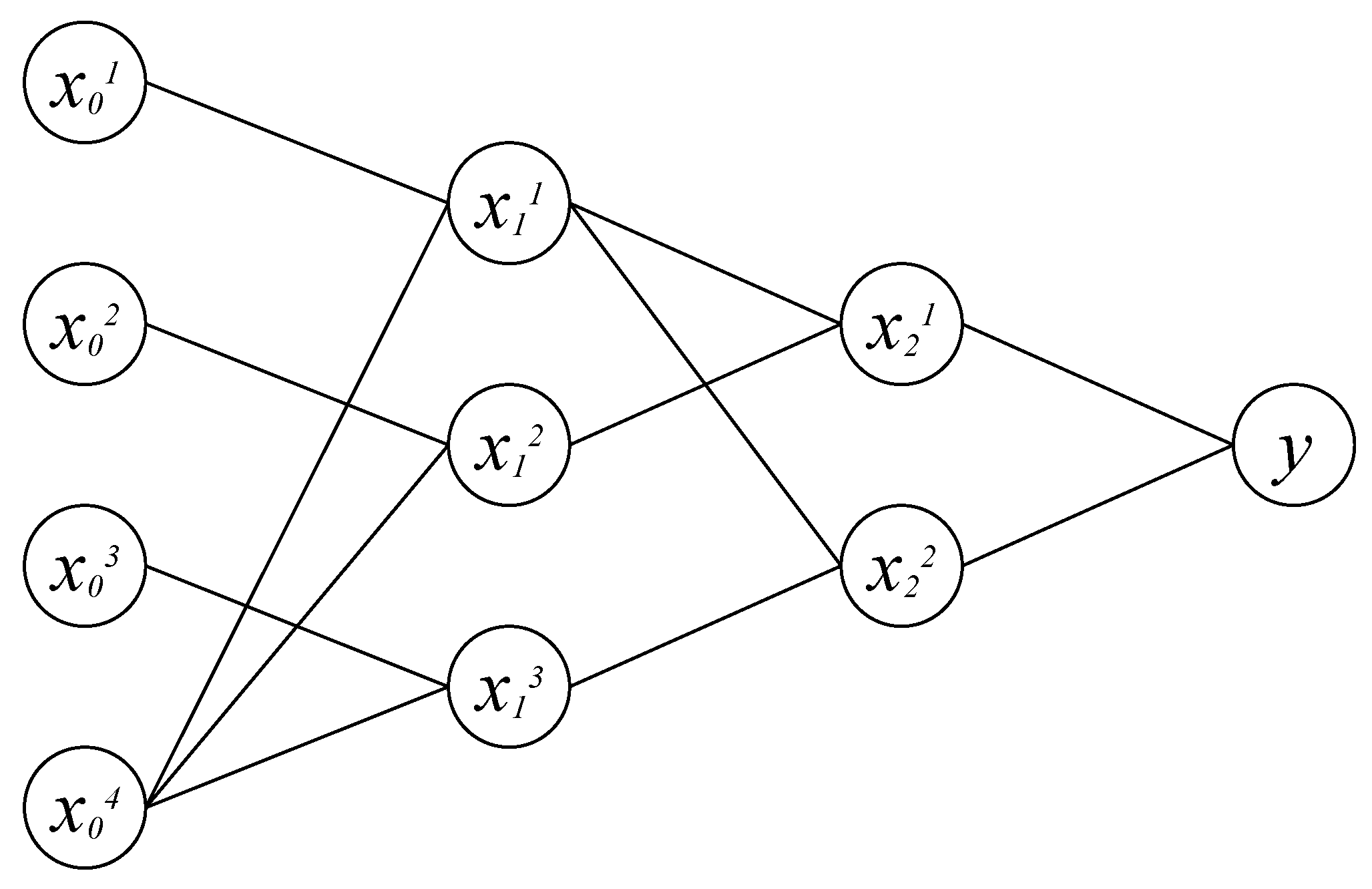
3.1. Group Method of Data Handling

The group method of data handling (GMDH) achieves self-organizing control of the data mining process and is a simple and efficient algorithm for deriving expressions for the original input variables of the optimal model and building an optimal complexity model in an objective way. Ghodsi and Khanjani [12] combined 697 experimental data to establish an equation for predicting scour depths based on the GMDH technique. The results show that the GMDH method can be applied to the scour depth prediction of complex bridge piers. The method is capable of modeling and predicting complex data systems based on certain input–output relationships [13]. The main idea is to establish an analytic function relationship between neural grids based on regression techniques.

In general, the relationship between the output and input quantities in the GMDH algorithm can be expressed as a Kolmogorov–Gabor function [14]. Furthermore, retaining terms only up to the quadratic terms, the relationship between the output and input quantities can be simplified to the following form [14]:

$$\widehat{y}=a_0+{\displaystyle \sum _{i=1}^n{a}_i{x}_i+{\displaystyle \sum _{i=1}^n{\displaystyle \sum _{j=1}^n{a}_{ij}{x}_i{x}_j}}}$$

(10)

where y is the output quantity, a is the weighting factor, z is the input quantity.

Based on the standard orthogonal least squares principle, the weight coefficients w of the GMDH model can be expressed as

$$a={(X^{T}X)}^{-1}{X}^{T}Y$$

(11)

$$X=\left[\begin{array}{llllll}1& x_{1p}& x_{1q}& x_{1p}{x}_{1q}& x_{1p}^2& x_{1q}^2\\ 1& x_{2p}& x_{2q}& x_{2p}{x}_{2q}& x_{2p}^2& x_{2q}^2\\ \hfill ⋮\hfill & \hfill ⋮\hfill & \hfill ⋮\hfill & \hfill ⋮\hfill & \hfill ⋮\hfill & \hfill ⋮\hfill \\ 1& x_{mp}& x_{mq}& x_{mp}{x}_{mq}& x_{mp}^2& x_{mq}^2\end{array}\right]p,q\in \left\{1,2,\dots ,n\right\}$$

(12)

$$Y={\left\{y_1,y_2,\dots ,y_m\right\}}^T$$

(13)

where m denotes the number of data, n denotes the number of input quantities.

3.2. GMDH Model Building

Whitenhouse [15] considers that the depth of local scour of offshore wind monopile foundations is related to factors such as current, seabed particles, and pile size.

$$S=f\left(D,d_{50},{\rho }_s,{\rho }_w,g,u_w,u_c,\nu ,h,H,L\right)$$

(14)

where f is the functional form, ρ_s is the sediment particle density, ρ_w is the current density, v is the current motion viscosity coefficient, L is the wavelength, u_w is the maximum flow velocity near the bottom of the wave, u_c is the average flow velocity at the current section.

In general, the eleven parameters related to the scour depth S were reduced to seven dimensionless parameters according to the Berkingham π theorem with D, h, and g as the basic parameters [16].

$$\frac{S}{D}=f\left(F{r}_a,Re,\frac{L}{D},\frac{L}{h},\frac{H}{h},\frac{d_{50}}{D},\frac{{\rho }_s}{{\rho }_w}\right)$$

(15)

where Fr_a is the Froude number corresponding to the average velocity of the wave action, Re is the pile Reynolds number, Re = u_c D/v, L/h is the ratio of wavelength to water depth, L/D is the ratio of wavelength to pile diameter, H/h is the ratio of wave height to water depth, d₅₀/D is the ratio of median sediment particle size to pile diameter, ρ_s/ρ_w is the ratio of sediment particle density to water density.

Qi and Gao [8] analyzed the local scour characteristics of monopiles under combined wave and current action by wave flow flume tests and obtained the average velocity of the water flow corresponding to the Froude number.

$$F{r}_a=u_a/\sqrt{gD}$$

(16)

Ettema et al. [17,18] concluded that the Froude number is closely related to the formation of a horseshoe vortex in front of the pile, which is an important cause of pile scour. In addition, Debnath and Chaudhuri [18] established a local scour prediction equation related to the Froude number. Thus, the Froude number is related to the variation of flow field around the pile perimeter under the combined wave flow action. In other words, the Froude number is a key factor leading to pile scour.

Moreover, Nielsen and Hansen [19] state that wave height, wave period, and water depth are the main factors affecting the maximum velocity of waves near the bottom under wave action. This will further affect the frictional flow velocity and shear stress of the sediment particles at the seabed surface, and ultimately the formation of scour holes at the seabed surface. Therefore, the wave parameters L/h and H/h can be used as influencing factors in the analysis of local scouring of monopiles.

Whitehouse [15] concluded that pile size has a significant effect on the flow field distribution around the pile. This was demonstrated by Qi and Gao [8] in a flume test under the wave–current condition.

Sumer and Fredsøe [6] concluded that turbulence occurs around the pile under the wave–current condition. The effect of Reynolds number on the local scour depth of the pile base is small and the effect of Reynolds number can be ignored.

Melville and Chiew [20] concluded that sediment grain size has little effect on the maximum local scour depth when D/d₅₀ > 50. The scour data used in this paper all satisfy this condition and there is little difference in sediment particle density, so the effects of median sediment particle size and particle density are ignored. Therefore, Equation (14) can be rewritten as

$$\frac{S}{D}=f\left(F{r}_a,\frac{L}{h},\frac{H}{h},\frac{L}{D}\right)$$

(17)

In summary, the main influencing factors of local scour depth of monopile foundations under the wave–current condition are Fr_a, L/h, L/D, H/h. Therefore, the structure of the GMDH model established in this paper is shown in Figure 1, with the initial inputs x₀¹, x₀², x₀³, x₀⁴ as L/D, H/h, L/h, Fr_a, respectively. The model has 3 layers of neural grid and 6 neurons, x₁¹, x₁², x₁³, x₂¹, x₂², y, where y is the final prediction S/D of the model.

Therefore, the equation for predicting the local scour depth of pile foundations based on the GMDH model can be expressed as

$$\begin{array}{l}{x}_1^1=a_{11}+a_{12}F{r}_a+a_{13}\frac{L}{D}+a_{14}F{r}_a{}^2+a_{15}{(\frac{L}{D})}^2+a_{16}F{r}_a\cdot \frac{L}{D}\\ x_1^2=a_{21}+a_{22}F{r}_a+a_{23}\frac{H}{h}+a_{24}F{r}_a{}^2+a_{25}{(\frac{H}{h})}^2+a_{26}F{r}_a\cdot \frac{H}{h}\\ x_1^3=a_{31}+a_{32}F{r}_a+a_{33}\frac{L}{h}+a_{34}F{r}_a{}^2+a_{35}{(\frac{L}{h})}^2+a_{36}F{r}_a\cdot \frac{L}{h}\\ x_2^1=a_{41}+a_{42}{x}_1^1+a_{43}{x}_1^3+a_{44}{(x_1^1)}^2+a_{45}{(x_1^3)}^2+a_{46}{x}_1^1\cdot x_1^3\\ x_2^2=a_{51}+a_{52}{x}_1^2+a_{53}{x}_1^3+a_{54}{(x_1^2)}^2+a_{55}{(x_1^3)}^2+a_{56}{x}_1^2\cdot x_1^3\\ y=a_{61}+a_{62}{x}_2^1+a_{63}{x}_2^2+a_{64}{(x_2^1)}^2+a_{65}{(x_2^2)}^2+a_{66}{x}_2^1\cdot x_2^2\end{array}$$

(18)

where a₁₁~a₆₆ are weighting factors.

3.3. Parameter Inversion

Qi and Gao et al. [8] conducted a series of physical model tests in sandy soils under coupled wave flow and found that the wave flow significantly changed the pore water pressure of the sediment around the pile, and verified that the horseshoe-shaped vortex was closely related to the formation of local scour pits. Li et al. [21] conducted a series of physical model tests to analyze the scouring of large-diameter monopile foundations under the action of wave flow on a sandy seabed and obtained a formula to predict the scour depth based on the test data.

Based on the experimental data of Qi et al. [8] and Li et al. [21], the results of the operation of the GDMH model and the weight coefficients of the input–output relationship of each neuron can be obtained. The fitting results and the fit are shown in

Table 1. Weighting coefficient fitting results.

Weighting Factor	a11	a12	a13	a14	a15	a16
Fitting results	−0.559	3.634	2.672	2.264	−2.203	−9.738
Goodness of fit R2	0.9012
Weighting factor	a21	a22	a23	a24	a15	a26
Fitting results	−0.315	−0.055	0.093	4.309	−0.012	0.123
Goodness of fit R2	0.9016
Weighting factor	a31	a32	a33	a34	a35	a36
Fitting results	−0.005	1.156	−0.004	0.69	0	0.039
Goodness of fit R2	0.9112
Weighting factor	a41	a42	a43	a44	a45	a46
Fitting results	−0.014	0.918	−0.097	−1.69	−0.593	2.257
Goodness of fit R2	0.9235
Weighting factor	a51	a52	a53	a54	a55	a56
Fitting results	0.009	0.501	0.394	−0.179	0.089	0.171
Goodness of fit R2	0.9097
Weighting factor	a61	a62	a63	a64	a65	a66
Fitting results	−0.022	1.42	0.128	−31.041	−15.837	44.211
Goodness of fit R2	0.9165

, and the fitting effects are shown in Figure 2. From the fitting results, it can be found that the fitting degree of each weight coefficient is above 0.9, which represents a good fitting result.

In order to quantitatively analyze the variability and applicability of local scour calculation methods, four statistical indicators are used in this paper, relative error (ε_r), mean relative error (ε_a), variance (δ_e), and normalized variance (δ_en).

$${\epsilon }_r=\frac{\left|S_y-S_c\right|}{S_c}\times 100\%$$

(19)

$${\epsilon }_a=\frac{1}{n}{\displaystyle \sum _1^n\frac{\left|S_y-S_c\right|}{S_c}}\times 100\%$$

(20)

$${\delta }_e=\frac{{\displaystyle \sum {(S_y-S_c)}^2}}{{\displaystyle \sum S_c{}^2}}\times 100\%$$

(21)

$${\delta }_{en}=\frac{{\displaystyle \sum {(S_y/D-S_c/D)}^2}}{{\displaystyle \sum {(S_c/D)}^2}}\times 100\%$$

(22)

where S_y represents the calculated value of the scour prediction equation, S_c represents the measured value of the scour depth, and n represents the number of data.

4. Case Studies

4.1. Case One: Monopile Scouring Flume Test

4.1.1. Test Overview

The test was conducted at the Nanjing Hydraulic Research Institute. As shown in Figure 3, the test flume was 175 m long, 1.2 m wide, and 1.6 m high, with transparent tempered glass on both sides, fixed by channel steel, and a concrete slab at the bottom. The two-dimensional wave-making system of the tank adopts a flat pushing wave-making plate with a maximum amplitude of ±300 m, a maximum wave height of 0.35 m, a wave period of 0.5–6.0 s, and a wave surface amplitude of 1–30 cm. Waves with different wave heights and wave periods can be generated by controlling the wave maker. The water flow is mainly generated by a two-way pump with a rated flow rate of 0.5 m³/s and a maximum head of 2.7 m, which can generate two-way water flow. The incoming flow rate can be adjusted by the control valve to control the flow rate required for different test conditions.

4.1.2. Model Sand Selection

Zhou [22] assumed that for any clayey soil composed of specific soil grains, there exists an objectively cohesion-less soil with comparable scour resistance. Therefore, according to the similar conditions of sediment initiation, a suitable model sand can be selected to simulate the local scouring characteristics of clayey soil.

In general, the model sand commonly used in the water tank test includes heavy, medium, and light model sand. Heavy model sand includes natural sand, fly ash, and talcum powder. Medium model sand includes coal, Bakelite powder, synthetic plastic sand, walnut shells, etc. Light model sand includes plastic sand, wood chips, asphalt wood chips, etc. Of these model materials, the properties of coal dust are particularly well suited to the needs of our flume experiment. This is because coal dust has a particle shape similar to natural sand, with a wide range of particle sizes (0.06–5 mm) and stable properties, and it is less susceptible to deterioration. In addition, coal dust has the advantages of large resting angle under water, mass production, low price, and wide applicability. Therefore, coal dust is widely used in physical model flume tests and has been proven to be a good choice for model sand [23]. Coal dust was selected as the model sand in this test. The median particle size d₅₀ of the selected coal dust was 0.65 mm and the particle bulk weight γ_s = 1.35 t/m³.

Zhang et al. [24] combined a large number of indoor tests and field measurement data to obtain a unified starting speed calculation formula applicable to viscous and non-viscous sands. The formula is as follows.

$$u={\left(\frac{h}{d_{50}}\right)}^{0.14}\sqrt{17.6\frac{{\gamma }_s-\gamma }{\gamma }{d}_{50}+6.05\times {10}^{-7}\frac{10+h}{d_{50}^{0.72}}}$$

(23)

where u is the sediment starting flow velocity, d₅₀ is the median particle size of sediment particles, h is the water depth, γ_s is the capacitance of sediment particles, γ is the capacitance of water, which is taken as 1000 kg/m³ in this paper.

The selected model flume test water depth is 50 cm, and the corresponding model sand starting velocity is 0.18 m/s by applying the Zhang formula. The average starting velocity of seabed silty clay is 1.81 m/s, and the similarity ratio calculation results are shown in

Table 2. Similarity scale calculation results.

Pile Diameter Scale λD	Prototype		Models		Starting Speed Similarity Ratio λu	Model Similarity φ (%)
	Water Depth hp (m)	Starting Speed up (m/s)	Water Depth hm (m)	Starting Speed um (m/s)
100	10	1.81	0.5	0.18	10.06	101

. The model similarity φ in this paper is defined as follows.

$$\phi =\frac{Z_m}{Z_p}\times 100\%$$

(24)

where φ is the model similarity, Z_m is the model physical quantity, Z_p is the prototype physical quantity.

4.1.3. Model Layout

Whitehouse [25] argues that the effect of the flume sidewalls on the local scour depth of the pile foundations can be ignored when the wave flow flume width B and pile diameter D satisfy B/D ≥ 6. The maximum pile diameter D in this test is 0.2 m, which satisfies this condition. Ettema [26] suggests that the effect of sediment grain size can be ignored when the pile diameter D and the sediment median grain size d₅₀ satisfy D/d₅₀ > 50. The median particle size d₅₀ of coal dust used in this test is 0.63 mm, and the minimum pile diameter D is 0.08 m. D/d₅₀ is much larger than 50 and meets this condition. Gudavalli [27] argues that the effect of water depth can be ignored when the water depth h and pile diameter D satisfy h/D ≥ 1.6. In this test, the water depth h is maintained at 0.5 m and the maximum pile diameter is 0.2 m. h/D = 2.5 > 1.6, satisfying this condition.

The model pile is a transparent Plexiglas pipe pile with a length of 1000 mm. As shown in Figure 3, the diameters of the two pile foundations are 100 mm and 200 mm, respectively, and the wall thickness is 10 mm. Three Doppler velocimeters (ADVs) were installed at 0.5 m in front of the piles to measure the flow velocity variation in front of the piles. Three wave height meters were positioned 1 m in front of the pile to measure the wave height variation during the test. A camera was built into the Plexiglas pile to measure the local scour depth around the pile.

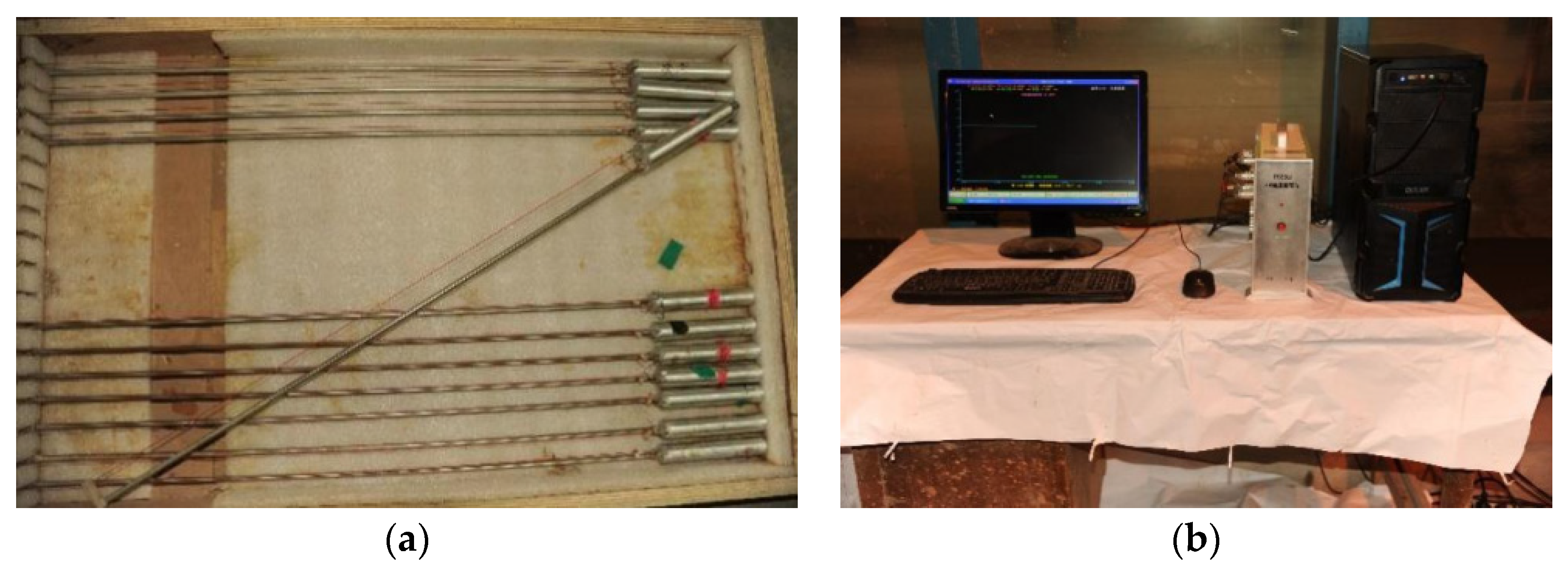
4.1.4. Measuring Systems

Flow velocity measurement. As shown in Figure 3, the acoustic Doppler velocimeter (ADV) was placed 0.5 m in front of the pipe. As shown in Figure 4a, the acoustic Doppler velocimeter (ADV) can accurately measure the water velocity in the range of 0.01~3 m/s with an accuracy of 0.1 mm/s. Combined with the flow velocity collector and collection system shown in Figure 4b, the flow velocity was measured.

Wave element measurement. As shown in Figure 3, the wave height meter was placed 1 m in front of the pipe pile. As shown in Figure 4a, the DS30 64-channel wave height meter developed by Nanjing Hydraulic Research Institute was used. Combining the wave height collector and collection system shown in Figure 4b, wave characteristic parameters such as maximum wave height, average wave height, 1/3 large wave height, 1/10 large wave height, and wave number were obtained.

Local scour depth measurement. The local scour depth measurement around the pile perimeter was carried out using an underwater HD endoscope. The scour depth was read by the camera after the scour was completed.

4.1.5. Test Results

Figure 5 shows the formation of scour pits. Numerous experimental studies have shown that the local scour depth around the pile is maximum when the wave flow is in the same direction [8,28]. Therefore, the same direction was used for the waves and currents created in this test. A total of 18 sets of scour tests were carried out for 0.1 m small-diameter pile foundations and 0.2 m large-diameter pile foundations under the joint action of wave and current. The test parameters and test results are shown in

Table 3. Wave scour test parameters.

Group	Pile Diameter D (m)	Wave Height H (m)	Cycle Time T (s)	uc (m/s)	uwm (m/s)	um (m/s)	ucw (m/s)	S/D
1	0.1	0.045	1.2	0.211	0.064	0.275	0.77	0.83
2	0.1	0.065	1.2	0.211	0.081	0.292	0.72	0.81
3	0.1	0.12	1.2	0.211	0.119	0.33	0.64	0.8
4	0.1	0.06	2	0.142	0.081	0.223	0.64	0.76
5	0.1	0.089	2	0.096	0.103	0.199	0.48	0.43
6	0.1	0.089	2	0.104	0.103	0.207	0.50	0.56
7	0.1	0.089	2	0.142	0.103	0.245	0.58	0.66
8	0.1	0.15	2	0.104	0.181	0.285	0.36	0.46
9	0.1	0.15	2	0.131	0.181	0.312	0.42	0.56
10	0.2	0.045	1.2	0.226	0.063	0.289	0.78	0.6
11	0.2	0.065	1.2	0.226	0.091	0.317	0.71	0.57
12	0.2	0.12	1.2	0.226	0.153	0.379	0.60	0.62
13	0.2	0.06	2	0.157	0.082	0.239	0.66	0.27
14	0.2	0.089	2	0.118	0.115	0.233	0.51	0.11
15	0.2	0.089	2	0.119	0.115	0.234	0.51	0.14
16	0.2	0.089	2	0.157	0.115	0.272	0.58	0.27
17	0.2	0.15	2	0.119	0.178	0.297	0.40	0.12
18	0.2	0.15	2	0.155	0.178	0.333	0.47	0.17

Note: U_c is the constant flow velocity at D/2 from the bed, U_wm is the amplitude of wave-induced flow velocity at the water quality point at D/2 from the bed, U_cw is the flow velocity ratio, reflecting the proportion of constant flow, U_m is the maximum flow velocity at the water quality point caused by wave superposition at D/2 from the bed.

.

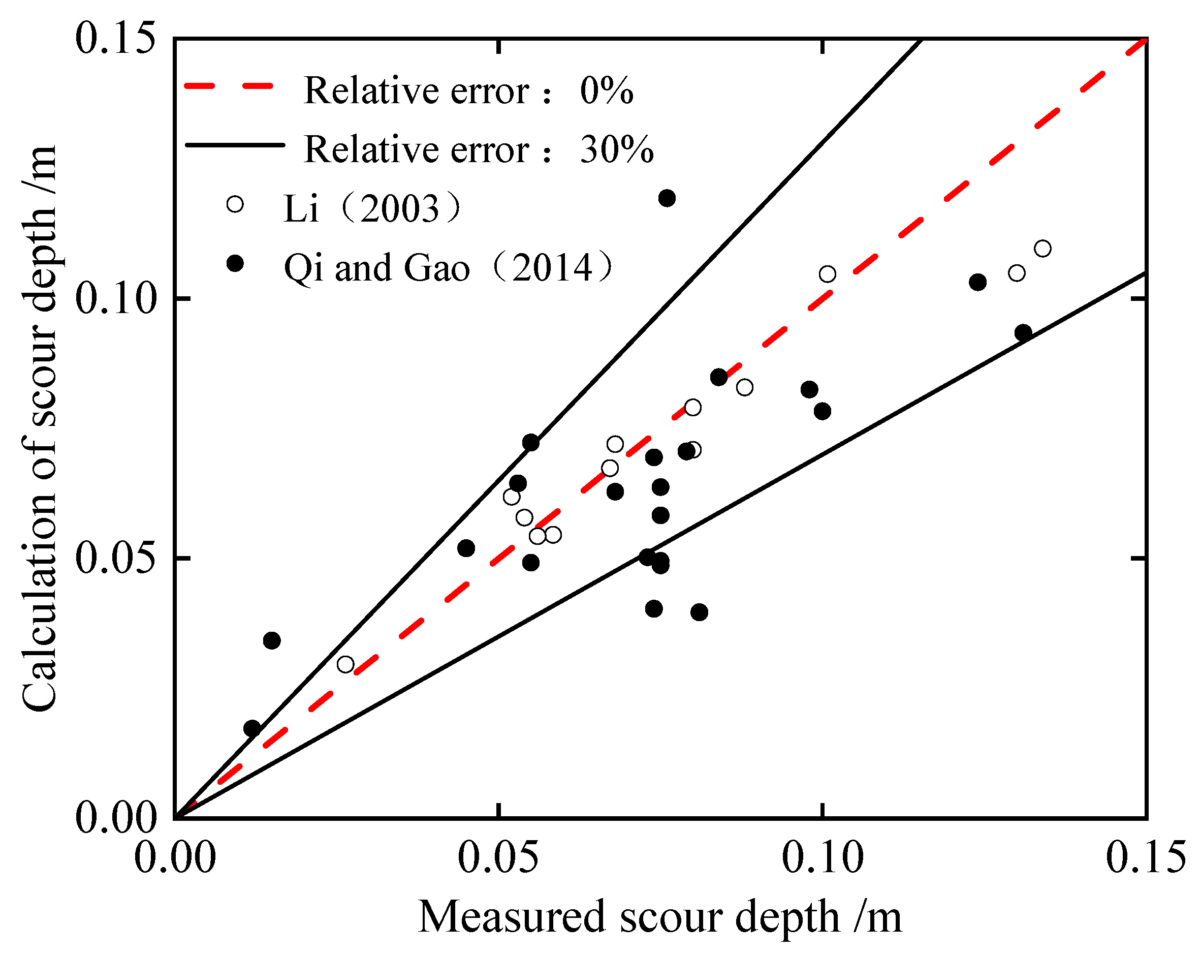
4.1.6. Analysis of Results

The relative errors between the measured and calculated values of the scour depth are shown in Figure 6. The horizontal coordinate of each point in the figure corresponds to a measured scour depth. The vertical coordinates of the points are the calculated values obtained by bringing the parameters corresponding to the measured scour depth (wave height, period, pile diameter, etc.) into the calculation formula. In order to compare the applicability of different formulas, it is necessary to use the same set of measured data. As can be seen from the figure, the points on the different plots correspond to the same horizontal coordinates. This also means that the measured scour depth is the same for the different formulas used.

It can be seen from the figure that the calculated and measured values of the prediction formulas in this paper are relatively evenly distributed, with most of them concentrated around the 1:1 slope line. Compared with the measured values of scour depth, the error of the calculated values using the prediction formulas in this paper is basically within the range of 50%. However, the calculated value deviations of the 65-1 correction formula and the 65-2 formulas are too large, and the error with the measured values is too large, so they are not analyzed in this paper. Furthermore, the calculated values of the HEC-18 formula, DNV specification formula, and Rudolph formula are much larger than the measured values, and the relative errors are above 50%, indicating that the calculated results are too safe. The dispersion of the calculated values of the Raaijmakers formula is large, indicating that the correlation between the calculated results of the formula and the measured data is poor.

The average relative errors ε_a, variance δ_e, and normalized variance δ_en of the calculated and measured values of each formula are shown in

Table 4. Scouring depth error statistics.

Type of Error	This Paper’s Formula	HEC-18 Formula	DNV Code Formula	Rudolph Formula	Raaijmakers Formula
Mean relative error εa	27.09	229.32	316.82	160.52	95.60
Variance δe	25.71	214.61	474.56	122.14	68.35
Normalized variance δen	32.90	231.61	122.27	121.32	122.76

. The statistical results show that the applicability of the prediction formulas in this paper is better than other formulas and the percentage of data with errors within 50% of the calculated results of the prediction formulas is 61%. The errors of the calculated results of the 65-1 correction formula and the 65-2 formula all exceed 100%. For the HEC-18 formula, DNV canonical formula, Rudolph formula, and Raaijmakers formula, the relative errors are all above 50%. The average relative error of the prediction formula in this paper ε_a is 27.09%, the variance δ_e is 25.71%, and the normalized variance δ_en is 32.90%, which are all much smaller than for the other formulas.

4.2. Case Two: Rudong Offshore Wind Farm

4.2.1. Overview of the Project

As shown in Figure 7, the Rudong 300 MW offshore wind farm project is located in the offshore waters of Rudong County, Jiangsu Province. The center of the site is 23 km offshore and the seafloor topography is highly variable, with deep tidal trenches. The elevation of the site is between −16.9 and 0.6 m. The wind farm has an irregular quadrilateral shape. The sea area is about 10 km long from east to west, 8 km wide from north to south, with a planned area of 82 km² and a project scale of 300 MW. According to the measured data from hydrographic measurement points, the wave height in the field area is 1.5~3.0 m, the wave period is 4.5~6.5 s, the wavelength is 30~50 m, and the tidal current speed is 2.1–3.0 m/s [29]. According to a multibeam bathymetry system, the average local scour depth of the 38 pile foundations is 8.15 m [30]. Other relevant information of the project is shown in

Table 5. Information about the Rudong Wind Farm [31].

Pile Number	Pile Diameter D (m)	Median Particle Size d50 (mm)	Water Depth h (m)	Scouring Depth S (m)
1–9	6.5	0.125	5~6	7.5~12.5
10–14	6.1	0.125	4~5	12.5~15.5
15–18	6.1	0.125	6~7	4.0~8.5
19–25	6.5	0.125	5~7	5.4~12.4
26–29	6.5	0.125	5~6	5.6~8.7
30–38	6.1	0.125	6~7	3.1~10.1

.

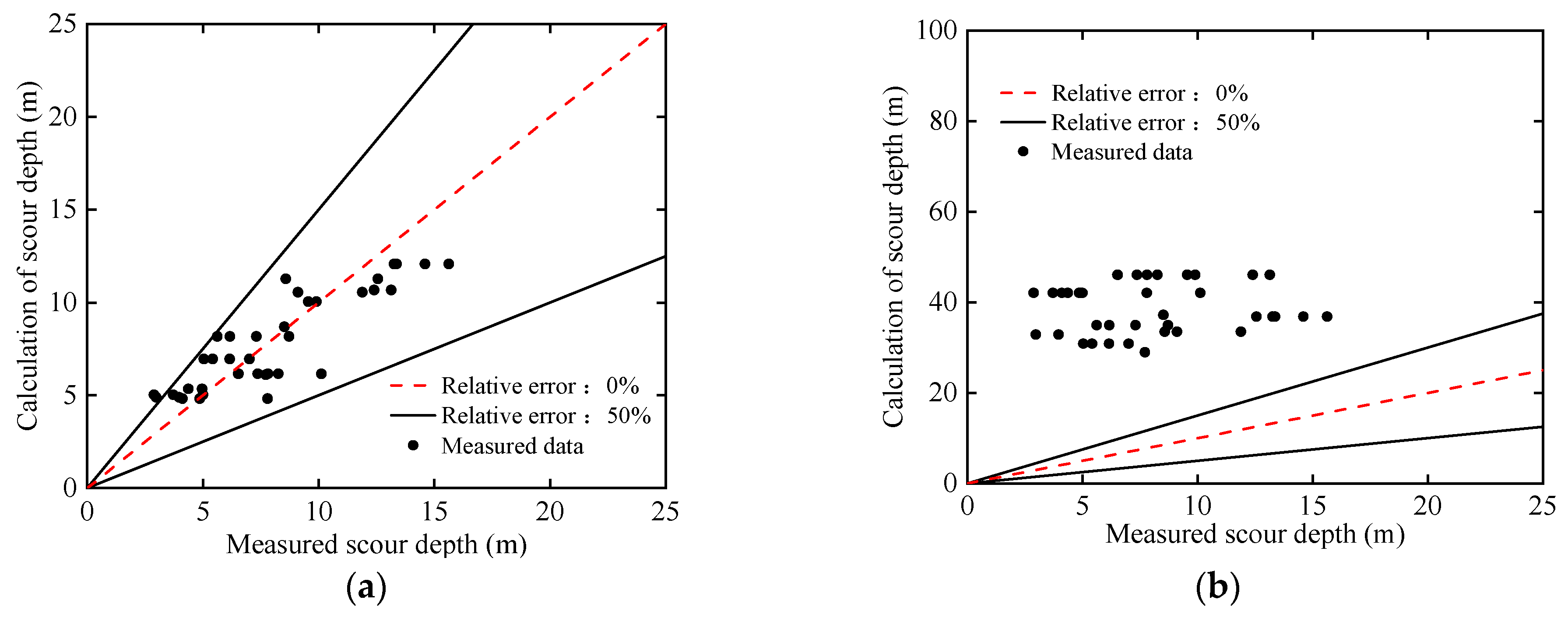
4.2.2. Analysis of Results

The relative errors between the measured and calculated values of the scour depth are shown in Figure 8. Similar to Figure 6, the horizontal coordinates of the points in Figure 8 are the actual measured values and the vertical coordinates are the values calculated by the formula.

It can be seen from the figure that the relative error between the calculated and measured values of the prediction formulas in this paper is not large and basically lies within the range of 50%.

The ratio between the calculated and measured values of formulas 65-1 and 65-2 lies between 100% and 200%, indicating that the calculated results are on the safe side.

The calculated values of the HEC-18 formula, DNV specification formula, and Raaijmakers formula differed very little, while the dispersion was large. In addition, the correlation between the calculated results of the three formulas and the measured data was poor.

Most of the values of the Rudolph formula are below the 1:1 diagonal line, indicating that the calculated results are on the dangerous side.

The mean relative error ε_a, variance δ_e, and normalized variance δ_en for the monitoring data are shown in

Table 6. Scouring depth error statistics.

Type of Error	This Paper’s Formula	65-1 Amendment formula	65-2 Formula	HEC-18 Formula	DNV Specification Formula	Rudolph Formula	Raaijmakers Formula
Mean relative error εa	18.31	243.77	128.97	42.77	49.42	39.28	42.32
Variance δe	12.31	323.90	164.28	27.47	23.51	23.23	32.71
Normalized variance δen	10.41	263.61	164.01	11.21	25.52	27.49	13.32

. The statistical results show that the prediction formula in this paper is more applicable, with 95% of the data within 50% of the error range. In contrast, all the calculated results for the 65-1 correction formula have an error of more than 50%. For the 65-2 formula, the percentage of data with errors within the 50% range is only 24%. For the HEC-18 formula, the DNV specification formula, the Rudolph formula, and the Raaijmakers formula, the proportion of data with errors within the 50% range is around 52%. The average relative error ε_a is 18.31%, the variance δ_e is 12.31%, and the normalized variance δ_en is 10.41% for the prediction formulas in this paper, all of which are much smaller than for the other formulas.

4.3. Reason for Higher Accuracy

The prediction formula in this paper performs better than the other formulas. This is because the GMDH method achieves self-organizational control of the data mining process. It builds an optimal complexity flush depth model in an objective manner. In addition, the initial inputs chosen in the process of building the model are Fr_a, L/h, L/D, and H/h. These four inputs mostly cover the important factors affecting the scour depth. Furthermore, Fr_a is considered as the core parameter affecting the scour depth. In the construction of the model, Fr_a is considered to be related to the other three input quantities at the same time. This is likewise an important reason for the high accuracy of the equations in this paper.

5. Conclusions

In this paper, a method for predicting local scour depth is investigated for offshore wind power monopile foundations and analyzed in comparison with existing calculation methods.

(1)

Based on the gauge analysis method and the group method of data handling (GMDH), considering the main influencing factors of the local scour depth of pile foundations and combining them with the existing experimental data, the prediction formula of the local scour depth of a single pile applicable to the action of wave flow is proposed.

(2)

Combining the flume test data and the scour monitoring data of Rudong Wind Farm in Jiangsu, the calculated values of the predicted depth of the existing calculation formulas and the calculated values of the prediction formula in this paper were compared. The results show that the formula in this paper has a higher calculation accuracy compared with other formulas.

Therefore, the formula in this paper has practical application value. It can calculate the scour depth around the pile foundation more accurately. This will play an extremely critical role in the design of monopile foundations for offshore wind turbines.

References

1. Richardson, E.V.; Harrison, L.J.; Richardson, J.R.; Davis, S.R. Evaluating Scour at Bridges, Second Edition (Reannouncement). Highw. Bridg. 1993, 23, 262. [Google Scholar]
2. JTG C30—2002; Hebei Provincial Transportation Planning and Design Institute: Specification for Hydrological Survey and Design of Highway Projects. People’s Traffic Publishing House: Beijing, China, 2002.
3. Veritas, D.N. Offshore Standard DNV-OS-J101; Design of Offshore Wind Turbine Structures; Submarine Pipeline Systems: Oslo, Norway, 2007. [Google Scholar]
4. Zhu, Z.W.; Yu, P. Comparative Study between Chinese Code and US Code on Calculation of Local Scour Depth around Bridge Piers. China J. Highw. Transp. 2016, 29, 36–43. [Google Scholar]
5. Liang, F.; Wang, C.; Yu, X.B. Performance of Existing Methods for Estimation and Mitigation of Local Scour around Bridges: Case Studies. J. Perform. Constr. Facil. 2019, 33, 04019060. [Google Scholar] [CrossRef]
6. Sumer, B.M.; Fredsøe, J. Wave Scour around a Large Vertical Circular Cylinder. J. Waterway Port Coast. Ocean Eng. 2001, 127, 125–134. [Google Scholar] [CrossRef]
7. Zanke, U.C.E.; Hsu, T.W.; Roland, A.; Link, O. Equilibrium scour depths around piles in noncohesive sediments under currents and waves. Coast. Eng. 2011, 58, 986–991. [Google Scholar] [CrossRef]
8. Qi, W.G.; Gao, F.P. Equilibrium scour depth at offshore monopile foundation in combined waves and current. Sci. China Technol. Sci. 2014, 57, 1030–1039. [Google Scholar] [CrossRef] [Green Version]
9. Rudolph, D.; Bos, K. Scour around a monopile under combined wave-current conditions and low KC-numbers. In Proceedings of the 3rd International Conference on Scour and Erosion (ICSE-3), Amsterdam, The Netherlands, 1–3 November 2006. [Google Scholar]
10. Harris, J.M.; Whitehouse, R.; Benson, T. The time evolution of scour around offshore structures. Marit. Eng. 2010, 163, 3–17. [Google Scholar] [CrossRef] [Green Version]
11. Gao, D.G.; Wang, Y.L. Bridge and Culvert Hydrology, 5th ed.; People’s Traffic Publishing House: Beijing, China, 2016; pp. 138–165. [Google Scholar]
12. Shaghaghi, S.; Bonakdari, H.; Gholami, A.; Ebtehaj, I. Comparative analysis of GMDH neural network based on genetic algorithm and particle swarm optimization in stable channel design. Appl. Math. Comput. 2017, 313, 271–286. [Google Scholar] [CrossRef]
13. Ivakhnenko, A.G.; Ivakhnenko, G.A. The Review of Problems Solvable by Algorithms of the Group Method of Data Handling (GMDH). Pattern Recognit. Image Anal. 1995, 5, 527–535. [Google Scholar]
14. Najafzadeh, M.; Barani, G.A.; Kermani, M. Estimation of Pipeline Scour due to Waves by GMDH. J. Pipeline Syst. Eng. Pract. 2014, 5, 06014002. [Google Scholar] [CrossRef]
15. Whitehouse, R. Scour at Marine Structures: A Manual for Practical Applications; Thomas Telford Publishing: London, UK, 1998. [Google Scholar]
16. Zhang, W.J.; Liu, H.N. Hydraulics; China Construction Industry Press: Beijing, China, 2015; pp. 81–88. [Google Scholar]
17. Ettema, R.; Kirkil, G.; Muste, M. Similitude of Large-Scale Turbulence in Experiments on Local Scour at Cylinders. J. Hydraul. Eng. 2006, 132, 33–40. [Google Scholar] [CrossRef]
18. Debnath, K.; Chaudhuri, S. Laboratory experiments on local scour around cylinder for clay and clay–sand mixed beds. Eng. Geol. 2010, 111, 51–61. [Google Scholar] [CrossRef]
19. Nielsen, A.W.; Hansen, E.A. Time-Varying Wave and Current-Induced Scour around Offshore Wind Turbines. In Proceedings of the ASME 2007 26th International Conference on Offshore Mechanics and Arctic Engineering, San Diego, CA, USA, 10–15 June 2007. [Google Scholar]
20. Melville, B.W.; Chiew, Y.M. Time Scale for Local Scour at Bridge Piers. J. Hydraul. Eng. 1999, 125, 59–65. [Google Scholar] [CrossRef]
21. Li, L.P.; Zhang, R.X. Forecast of the maximum scour depth around vertical cylinders of large diameter combined wave and current action. J. Dalian Univ. Technol. 2003, 43, 5. [Google Scholar]
22. Zhou, M.D. Study on similarity of local scouring of cohesive material in hydraulic model test. ShuiliXuebao 1998, 4, 33–40. [Google Scholar]
23. Zhang, X.N.; Dou, G.R. Review of common model sands and their specific properties. Hydrosci. Eng. 1994, 15, 45–51. [Google Scholar]
24. Zhang, R.J.; Xie, J.H.; Chen, W.B. River Dynamics; China Industrial Publishing House: Beijing, China, 1961. [Google Scholar]
25. Whitehouse, R.; Harris, J.M.; Sutherland, J.; Rees, J. The nature of scour development and scour protection at offshore windfarm foundations. Mar. Pollut. Bull. 2011, 62, 73–88. [Google Scholar] [CrossRef] [Green Version]
26. Ettema, R. Scour at bridge piers. Depth 1980, 26, 527. [Google Scholar]
27. Gudavalli, S.R. Prediction Model for Scour Rate around Bridge Piers in Cohesive Soil on the Basis of Flume Tests; Texas A&M University: College Station, TX, USA, 1997. [Google Scholar]
28. Cheng, Y.Z.; Tang, W.; Li, D.L.; Huang, X.Y. Experimental study on local scour around the pile on the sandy seabed under wave action. Adv. Water Sci. 2018, 29, 9. [Google Scholar]
29. Yang, H.; Zhang, W. Simulation of Sediment erosion and silting on Rudong Offshore Wind Farm Project in Jiangsu province by MIKE21. Trans. Oceanol. Limnol. 2021, 43, 48–57. [Google Scholar]
30. Shang, J.; Zhao, Y.Y. Calculation Research on Local Scouring Depth of Pile Foundation of Intertidal Wind Power Unit. Wind. Energy 2016, 32, 90–92. [Google Scholar]
31. Hu, D.N. Dynamic Response Research for Offshore Wind Turbine Pile-Foundation and Superstructure Subjected to Wave Loads. Master’s Thesis, Chongqing Jiaotong University, Chongqing, China, 2014. [Google Scholar]
Figure 1. Schematic diagram of the GMDH model structure.
Jmse 11 00753 g001
Figure 2. Fitting effect of prediction formula.
Jmse 11 00753 g002
Figure 3. Diagram of the flume scour test.
Jmse 11 00753 g003
Figure 4. Measurement systems. (a) ADV, wave height meters. (b) Flow velocity and wave height acquisition systems.
Jmse 11 00753 g004
Figure 5. Local scour pit pattern around the pile.
Jmse 11 00753 g005
Figure 6. Comparison of calculated values and measured data for different scouring formulas in case one. (a) This study’s formula, (b) HEC-18 formula, (c) DNV specification formula, (d) Rudolph specification formula, (e) Raaijmakers specification formula.
Jmse 11 00753 g006aJmse 11 00753 g006b
Figure 7. Rudong Wind Farm: (a) sea area where the wind farm is located, (b) on-site scour pit cloud map.
Jmse 11 00753 g007
Figure 8. Comparison of calculated values and measured data for different scouring formulas in case two. (a) This paper’s formula, (b) 65-1 revised formal calculation method, (c) HEC-18 formula, (d) HEC-18 formula, (e) DNV specification formula, (f) Rudolph specification formula, (g) Raaijmakers specification formula.
Jmse 11 00753 g008aJmse 11 00753 g008b