Abstract
In this study, nondominated sorting genetic algorithm II (NSGA-II) was used to minimize the cost and carbon emissions of a liquefied natural gas (LNG) dual-fuel ship for a given route. This study considered the regulations of emission control areas (ECA) and the European Union (EU) Emissions Trading System (ETS) to determine the optimal speed and LNG/oil ratio for the ship. NSGA-II used the arrival time at each port and the LNG usage ratio for each voyage leg as its genes. The time window for arrival, the fuel cost, and potential EU carbon emission regulations were used to estimate the cost of the considered voyage. Moreover, fuel consumption was determined using historical data that were divided by period, machinery, and voyage leg. The results indicated that the optimal speed and fuel ratio could be determined under any given fuel and carbon price profile by using NSGA-II. Finally, the effects of regulations and carbon price differences on the optimal speed and fuel ratio were investigated. The cost minimization solution was susceptible to being affected by the regulations of ECAs and the EU ETS. The speed profile of the cost minimization solution was found to have a tendency to travel at faster-than-average speeds outside ECAs and non-EU regions, and travel slower in ECAs and EU regions. Meanwhile, the selection of fuel type showed that 100% traditional fuel oil in all regions, but with sufficiently high EU carbon permit cost, tends to use 100% LNG in EU regions.
1. Introduction
In 2018, the International Maritime Organization (IMO) set a goal to reduce greenhouse gas (GHG) emissions from ships by at least 50% by 2050 relative to the corresponding level in 2008 [1]. This goal is known as the IMO’s Initial GHG Strategy. However, the IMO is currently revising its Initial GHG Strategy and expects to finalize the revised strategy in 2023 [2]. To help meet the aforementioned goal, the IMO [3] has introduced several new measures, including the Energy Efficiency Existing Ship Index and Carbon Intensity Index (CII), for assessing the GHG emissions of ships and providing a basis for comparing the efficiency of different ships.
The European Union (EU) is also taking action to reduce GHG emissions from ships [4]. The EU is currently considering including the maritime sector in its Emissions Trading System (ETS). This inclusion would result in ship owners being required to pay for their GHG emissions at EU ports. This policy is expected to incentivize ships to become more efficient and emit less carbon [5]. In addition to the aforementioned measures, the IMO has introduced regulations to manage sulfur emissions from ships. These regulations have established sulfur emission control areas (ECAs) in which ships must use fuel with a sulfur content of no more than 0.1%. Outside of ECAs, ships can use fuel with a sulfur content of up to 0.5% [6]. In general, shipping companies tend to use cheap fuels unless relevant restrictions (e.g., ECAs and CII thresholds) or taxes (e.g., the EU ETS) exist. Overall, the aforementioned measures are creating new challenges for ship companies, which must now find methods to reduce their GHG emissions and comply with the new regulations while minimizing the impact on their profits.
Available alternative fuels for ships include liquefied natural gas (LNG), methanol, ammonia, and hydrogen. Smith et al. [7] predicted the fuel types that will be used in the future to achieve the goal of net-zero emissions by 2050, as shown in Figure 1. LNG is expected to replace traditional fuels, such as low-Sulfur fuel oil (LSFO) and marine diesel oil (MDO), and become the primary fuel in the near future. The use of ammonia is expected to grow considerably after 2030, and ammonia will become the dominant maritime fuel by 2050. According to Burel et al. [8], the usage of LNG may reduce carbon emissions by up to 25%. Therefore, an LNG dual-fuel ship was considered in the present study. An assumption was made that such a ship can be set to sail with any fuel ratio between 100% fuel oil and 100% LNG in the dual-fuel mode [9].
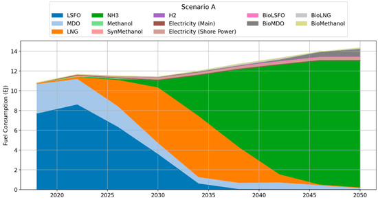
Figure 1.
Types of fuel predicted to be used to reach the goal of net-zero GHG emissions by 2050 [7].
According to Faber et al. [10], 44 methods exist for making ships more efficient. These methods can be divided into four groups: those involving the use of energy-saving technologies, the use of renewable energy, the use of alternative fuels, and speed reduction. In addition to these methods, operation optimization is crucial. Zis et al. [11] reviewed studies on weather routing and the conditions considered in these studies. In the aforementioned studies, the method used for estimating fuel consumption under a specific sailing speed involved three steps: environment impact prediction, power consumption prediction, and fuel consumption prediction. In the present study, the speed–fuel consumption relationship was obtained through the regression of historical data. Speed optimization is also a potential method for reducing GHG emissions from ships [12,13,14,15,16,17,18,19,20,21,22,23,24]. Ma et al. [12] investigated ship speed and route optimization by considering the rules of ECAs. De et al. [15] proposed a method to minimize the carbon emission and maximize the profit of the shipping company. The optimization variables considered in [15] were the ship routing and scheduling, loading/unloading operations, the time window concept at ports, and vessel draft restrictions. Fagerholt et al. [16] explored the speed optimization of single-fuel ships in a soft time window for a certain route. Wu et al. [17] linearized the complex, nonlinear cost minimizing problem by optimizing the fleet deployment, ship refueling strategies, and sailing speed of an LNG dual-fuel ship. Lu et al. [18] investigated the speed optimization while considering ECAs by Multiple Objective Particle Swarm Optimization (MOPSO). Han et al. [19] developed a speed optimization model that considered various policies and strategies, including the ECA policy, carbon tax policy, Vessel Speed Reduction Incentive Program, and virtual arrival strategy. Dulebenets [20] introduced speed and route optimization to minimize the cost while considering the carbon tax policy. Zhen et al. [21] established a bi-objectives optimization model to minimize the fuel cost and SO2 emission. The variables in the study were the ship route and speed. Li et al. [22] used the speed optimization to minimize the operating cost and the fuel consumption. Gao and Hu [23] optimized the speed and fleet deployment to minimize the total sailing cost. Zhuge et al. [24] introduced speed, path, and fleet deployment optimization to minimize the sailing cost by a dynamic programming-based algorithm. De et al. [25] discussed the bunker strategy and route optimization.
In summary, recent ship operating optimization research often combined speed with other variables, and the optimization objectives were often set to be carbon emission and sailing cost, as shown in Table 1. However, few papers considered the fuel ratio of the dual-fuel ship as an optimization variable. To fill this research gap, the present study applied the speed and fuel ratio optimization to an LNG dual-fuel ship. The optimization procedure was conducted for a given route to minimize the ship’s costs and carbon emissions while adhering to the latest regulations of ECAs and the EU ETS. The effects of the regulations on the optimization results were investigated by comparing several scenarios. This study may contribute to shipping companies by proposing an optimized scientific operation mode to minimize the economic impact of complying new regulations.

Table 1.
Sample of operation optimization papers and the objectives, variables, algorithms, ship types, and considered regulations in those papers.
2. Problem Description and Model Establishment
2.1. Problem Description
The optimization process consists of three steps: voyage planning, fuel consumption estimation, and speed and fuel ratio optimization. The first step in voyage planning involves establishing the intended route of the vessel and acquiring relevant historical information about the target ship. Determining the time window for each port of call, which includes the earliest and latest acceptable arrival time at a specific port, is essential. This time window can be determined from the port’s request, the current conditions, or the transportation demands of the shipping company. Other crucial factors to consider during voyage planning include the maneuvering time (the time required for the pilot to maneuver the ship in and out of the port), maneuvering distance (the distance traveled during the maneuvering time), and time at berth (the time for which the vessel is scheduled to stay at a specific berth). The maneuvering time and time at berth are assumed to be fixed, and the sailing period is the target period to be optimized.
To predict fuel consumption during a voyage, the relationship between the fuel consumption rate and ship speed must be considered. This relationship is often represented using a mathematical power curve, as shown in Figure 2. The dependence of the fuel consumption rate on different factors—such as the machinery being used (e.g., main engine, auxiliary engine, and boiler), the conditions of the voyage (e.g., sailing, maneuvering, and at berth), and the port-to-port legs of the voyage [26]—must also be considered. Moreover, the effects of weather and sea conditions on fuel consumption could be examined under different slip ratios. The different fuel consumption rates set for different voyage legs can be used to simulate differences in weather and loading conditions between these legs [27]. To account for the effect of ECAs on the LNG dual-fuel ship, the fuels considered were 0.1% sulfur fuel oil, 0.5% sulfur fuel oil, and LNG. Within ECAs, only 0.1% sulfur fuel oil and LNG were allowed, whereas outside ECAs, all three types of fuel could be used. However, in this study, the fuel options outside the ECAs were limited to either a combination of 0.1% sulfur fuel oil and LNG or a combination of 0.5% sulfur fuel oil and LNG.
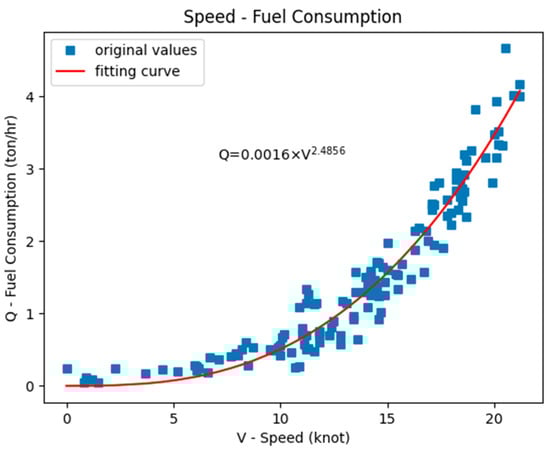
Figure 2.
Results of speed–fuel consumption regression for a dual-fuel ship.
The variables of NSGA-II, which are also known as genes, were the arrival time within the given time window of each port of call and the LNG/oil ratio of each leg. The two objectives of this algorithm were cost minimization and carbon emission minimization. After the arrival times and LNG/oil ratios of each voyage leg were determined, the fuel consumption was estimated. Finally, the two objectives were achieved using the estimated fuel consumption, current fuel prices, carbon permits, and fuel carbon factor (Figure 3). The nomenclature and abbreviations used to establish the numerical model are shown in Table 2.
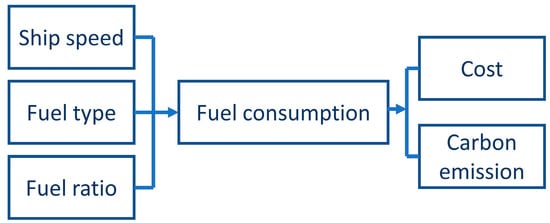
Figure 3.
Process for evaluating the costs and carbon emissions of a dual-fuel ship.
Table 2.
Nomenclature and list of abbreviations.
In summary, the assumptions in this study are as follows:
- 0.1% sulfur fuel oil only was always used in maneuvering and at berth periods;
- The ship speed was constant in a leg n;
- The fuel consumption and time in maneuvering and at berth periods were deterministic;
- In ECAs, 0.1% sulfur fuel oil and LNG could be used in any ratio;
- Outside ECAs, the combination of 0.1% S fuel oil and LNG or 0.5% S fuel oil and LNG could be chosen and used in any ratio;
- Fuel type index: i = 1 represented 0.1% sulfur fuel oil, i = 2 represented 0.5% sulfur fuel oil, and i = 3 represented LNG.
2.2. Optimization Algorithm
Nondominated sorting genetic algorithm II (NSGA-II) is an algorithm commonly used to find the set of optimal solutions, which is also known as the Pareto front (PF) or trade-off curve, for multi-objective optimization problems [28]. The procedure of NSGA-II comprises selection, crossover, mutation, nondominated sorting, and crowding distance calculation, as shown in Figure 4. The selection, crossover, and mutation are procedures of standard genetic algorithms. NSGA-II is famous for its high accuracy and convergence speed, and is validated by other studies [29,30,31,32]. In the present study, the NSGA-II of the pymoo package developed by Blank and Deb [33] in Python was used to solve the considered problem of simultaneous cost and emission minimization. In the case of single-fuel ships, cost and carbon emissions can be integrated into one objective, namely fuel consumption, because no trade-off exists between these objectives. Thus, a single optimal solution can be obtained. However, in the context of LNG dual-fuel ships, conflicting objectives exist because the use of LNG results in higher costs but lower emissions than does the use of traditional fuel oil. NSGA-II can find optimal solutions that optimize the conflicting objectives of cost and carbon emission for LNG dual-fuel ships. For these ships, the PF is a set of possible optimal solutions, one of which should be selected by the decision maker on the basis of additional information.
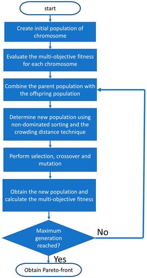
Figure 4.
Flowchart of NSGA-II [28].
As a genetic algorithm, NSGA-II comprises two crucial parameters: population size and number of generations. The population size is the number of agents that search for the optimal solution in the possible solution space, and the number of generations is the number of iterations for which the agents have searched the entire search space. The termination condition is usually set by limiting the number of generations. Increases in the population size and number of generations result in more accurate solutions; however, the computation process becomes longer. Therefore, for a complex problem with a larger possible solution space, NSGA-II with longer evaluation time is required to obtain acceptable optimized solutions. Determining an appropriate population size and number of generations for a problem can be challenging.
2.3. Mathematical Model
First, the fuel consumption model of each leg n and each fuel i should be established, as shown in Equations (1)–(6).
The ship’s speed and time of maneuvering period as well as the at-berth period were determined in the route planning process. The ship’s duration and speed of each leg of the sailing period were obtained from the estimated arrival time at each port of call, as shown in Equations (1) and (2). Equation (3) was used to calculate the fuel consumption of fuel i and leg n by summing up the fuel consumption of sailing, maneuvering, and at berth period of leg n. Equation (4) describes the three fuel types consumption of sailing period. Equations (5) and (6) represent the 0.1% sulfur fuel oil consumption of the maneuvering and at berth period for leg n, respectively.
Finally, the aforementioned constrained bi-objective problem can be expressed using Equations (7)–(13).
Equation (7) consists of arrival times and LNG/oil ratios for each leg. Equation (8) minimizes the total carbon emission. Equation (9) was used to obtain the carbon emission in the EU jurisdiction. Equation (10) was used to minimize the total sailing cost by summing up the fuel cost and the carbon permit cost. Equation (11) was used to guarantee that the arrival time of a port is later than the arrival time of the previous port. Equation (12) ensured the arrival time of a port was within the set time window. Equation (13) guaranteed that the LNG/oil ratio was between 100% fuel oil usage and 100% LNG usage.
3. Results and Discussion
The methodology outlined in the aforementioned text was adopted for a 4600-TEU container ship conducting a complete voyage. The itinerary considered commenced in Western Europe and proceeded to the eastern coast of North America through the Atlantic Ocean. The ship subsequently sailed back to Europe and concluded its journey at the starting port of call. The trip comprised nine ports of call, which included the initial and final ports, and four waypoints where oil changes occurred between ECAs and non-ECAs. Consequently, 12 legs had to be traversed, with 12 arrival times and 12 LNG/oil ratios to be determined. Data on the considered journey are presented in Table 3, Table 4 and Table 5, and a map of the considered route is displayed in Figure 5. The orange regions in Figure 5 indicated the ECAs.
Table 3.
Time windows and route in the considered example.
Table 4.
Assumed fuel properties: price, carbon factor, and lower calorific value for three different fuels.
Table 5.
Available fuel types in all legs and EU carbon permit costs set in four scenarios.
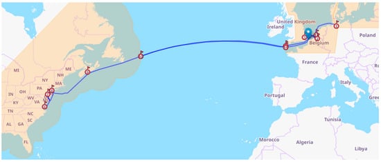
Figure 5.
Map of the considered route. Orange regions were considered ECAs.
In order to investigate the different optimal results of each consideration, the four scenarios were demonstrated and expressed in Table 5.
- General single fuel: using 0.1%-sulfur-containing fuel oil only in all legs and considering no EU ETS rules;
- General dual fuel: using 0.1%-sulfur-containing fuel oil and LNG in all legs and considering no EU ETS rules;
- Considering ECAs: using 0.1%-sulfur-containing fuel oil and LNG in ECAs, 0.5%-sulfur-containing fuel oil and LNG outside ECAs, and considering no EU ETS rules;
- Considering EU ETS: using 0.1%-sulfur-containing fuel oil and LNG in all legs and considering EU carbon permit of 100 or 200 USD/t-CO2;
All legs except leg 4 and 10 were assumed to be in ECAs, and legs 1–5 and 9–12 were assumed to be under the jurisdiction of EU ETS. The EU ETS was assumed to consider the 100% of carbon emission for legs 1–2 and 12, while considered 50% of carbon emission for legs 3–5 and 9–11. By comparing Scenario 1 with Scenario 2, the effects of using dual-fuel ships could be demonstrated. By comparing Scenario 2 with Scenario 3, the impacts of ECAs could be investigated. By comparing Scenario 2 with Scenario 4, the effects of the EU ETS could be determined. In these comparisons, Scenario 1 served as the control group when compared with Scenario 2, while Scenario 2 served as the control group when compared with Scenarios 3 and 4. The optimal speeds of Scenario 1 and 2 were also compared with the theoretical optimal speeds (average speed) for validation. Since Scenario 1 represented a general single-fuel ship, speed was the only variable being optimized.
3.1. Results for a General Single-Fuel Scenario and General Dual-Fuel Scenario
The set of optimal solutions could be presented in a two-objective figure and explained by the PF. In this study, the X-axis and Y-axis were set as cost and carbon emissions, respectively. The PF represents a set of optimal solutions for a problem. Each solution, which is represented by a point in the PF figures (Figure 6), comprised an arrival time and LNG/oil ratio. Because both minimization objectives were achieved simultaneously, solutions located further toward the bottom-left of the PF figures were better. For single-fuel ships, the PF was a single point (Figure 6a) because no trade-off existed between cost and carbon emissions. In this case, the optimal solution was the set of arrival times that minimized fuel oil consumption.
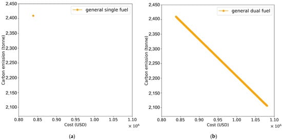
Figure 6.
PF figures for a (a) general single-fuel ship and (b) general dual-fuel ship. (a) The carbon emission and the cost had no trade-off on single-fuel ship; thus, it was one optimal solution and a single point on PF figure. (b) For the general LNG dual-fuel ship, the two objectives had conflicts, and the optimal solutions would become a straight line.
In contrast to the PF of a single-fuel ship, the PF of a general LNG dual-fuel ship was a straight line (Figure 6b) when the regulations of ECAs and the EU ETS were not considered. For an LNG dual-fuel ship, all solutions had similar arrival times but different LNG/oil ratios. The optimized solution that achieved the lowest cost, which was located in the top-left corner of the PF, corresponded to the use of fuel oil but no LNG (100% fuel oil). By contrast, the optimized solution that achieved the lowest carbon emission, which was located in the bottom-right corner of the PF, corresponded to the use of LNG but no fuel oil (100% LNG).
In the considered examples, the weather conditions and fuel consumption in a journey leg were assumed to be constant; therefore, the theoretical optimal sailing speed of the general single-fuel ship and general dual-fuel ship were the average speed for all the legs. However, NSGA-II is an evolutionary algorithm and can only search for the approximate optimal solution, as shown in Figure 7. It theoretically takes infinite time to obtain the exact average speed profile.
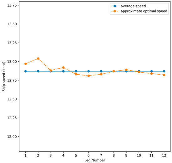
Figure 7.
Theoretical average speed (blue, solid line) and approximate optimal speed (orange, dash-dotted line) in all legs for both a general single-fuel ship and a general dual-fuel ship.
3.2. Effects of Emission Control Areas
When the regulations of ECAs were considered, available fuel oil could be divided into two categories: fuel oil with 0.1% and 0.5% sulfur. In the considered example, a mixture of 0.1%-sulfur-containing fuel oil with LNG could be used in the ECAs, whereas a mixture of 0.5%-sulfur-containing fuel oil with LNG could be used outside the ECAs (as shown in legs 4 and 10 of Scenario 3, Table 5). The optimization results indicated that the PF was bilinear when the aforementioned regulations were considered (Scenario 3, green solid line in Figure 8). The cost minimization solution corresponded to the use of only 0.1%-sulfur-containing fuel oil in the ECAs and only 0.5%-sulfur-containing fuel oil outside the ECAs. By contrast, the carbon minimization solution corresponded to the use of only LNG inside and outside the ECAs. The aforementioned results were obtained because the price of LNG is considerably higher than the prices of 0.1%-sulfur-containing fuel oil and 0.5%-sulfur-containing fuel oil. At the bending point of the bilinear PF (green-frame arrow in Figure 8), the solution corresponded to the use of only 0.5%-sulfur-containing fuel oil in non-ECAs and only LNG in ECAs. The optimal strategy involved substituting LNG with 0.1%-sulfur-containing fuel oil in the ECAs first, since 0.5%-sulfur-containing fuel oil is more cost-effective than is 0.1%-sulfur-containing fuel oil.
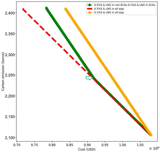
Figure 8.
PFs (green solid, orange solid, red dashed) represent Scenario 3, Scenario 2, and considering 0.5% sulfur oil and LNG available in all legs, respectively. The green-frame arrow indicates the bending point of green PF.
The speed profile also changed when considering the regulations of the ECAs (Figure 9). The cost minimization solution contained a marginally higher sailing speed outside the ECAs than did the carbon minimization solution. This result was obtained because 0.5%-sulfur-containing fuel oil is cheaper than 0.1%-sulfur-containing fuel oil. The carbon minimization solution had an average speed profile.
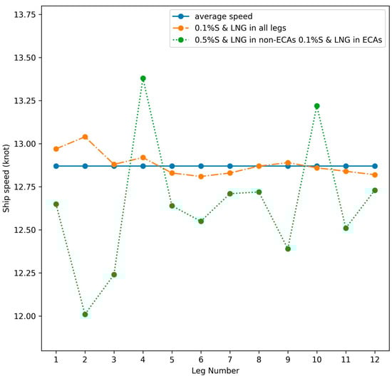
Figure 9.
Theoretical average speed (blue, solid line), cost minimization optimal speed (orange dashed dotted line and green dotted line) in all legs represent the Scenario 2 and Scenario 3.
3.3. Effects of the European Union Emissions Trading System
The rules of the EU ETS might also affect the optimal speed profile and fuel ratio. The EU carbon permit is assumed to be 100 or 200 USD/ton; as a result, the PFs were moved to the right, as shown in Figure 10. Consideration of these rules might result in marginal reductions in ship speed in areas under the 100% jurisdiction of the EU ETS (legs 1, 2, and 12 in Table 5) to reduce the cost incurred for EU carbon permits. Therefore, the cost optimal ship speed outside the EU would increase to comply the set time window, as shown in Figure 11. The bottom-right solution was the carbon emission minimization solution and thus still represented the average speed profile. Moreover, the cost minimization solution still involved the use of 100% fuel oil, whereas the carbon minimization solution involved the use of 100% LNG.
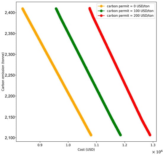
Figure 10.
PFs (orange, green, red) represent scenario 2, scenario 4 with a 100 USD carbon permit, and scenario 4 with a 200 USD carbon permit, respectively.
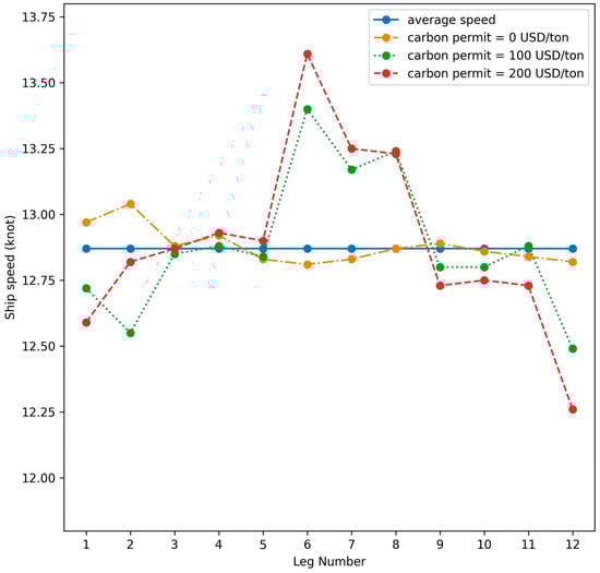
Figure 11.
Theoretical average speed (blue solid line), cost minimization optimal speed (orange dashed dotted line, green dotted line, and red dashed line) in all legs represent Scenario 2 and Scenario 4 with a 100 USD carbon permit, and Scenario 4 with a 200 USD carbon permit, respectively.
These effects may vary with the costs of each fuel and the EU carbon permit. For example, if the EU carbon permit cost is considerably higher than its current cost, the cost minimization solution would not exclude the use of LNG. This solution would involve the use of 100% LNG near EU ports and 100% fuel oil outside EU ports because the EU carbon permit cost is sufficiently high to cover the price gap between fuel oil and LNG. Equation (14) was used to determine whether the cost minimization solution involves the use of LNG. This equation compares the costs (including the costs for the fuel and carbon permit) of producing one unit of energy with fuel oil and LNG. If the carbon permit cost is sufficiently high to cause the cost of LNG to be less than that of fuel oil for producing one unit of energy, the cost minimization solution includes the use of LNG.
NSGA-II can be used to determine the optimal solutions under all conditions.
3.4. Convergence Analysis
NSGA-II obtained the approximate optimized solutions of the considered problem. Without a sufficient number of generations, the solutions might not converge and might be unsatisfactory. Many methods have been proposed to evaluate the convergence of solutions for multi-objective optimization problems. The simplest method involves comparing the PF of the current generation with that of the previous generation and examining whether the PF has shifted to the bottom-left of the PF figures. The shift of the PF can be represented as a hypervolume index [35]. When no considerable improvement occurs in the solution quality of the algorithm after an iteration, the results are considered to have converged. As displayed in Figure 12, the solutions of the considered problem converged after 250,000 function evaluations (500 generation and 500 population size) when using NSGA-II.
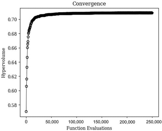
Figure 12.
Hypervolume analysis of the considered problem.
3.5. Sensitivity Analysis
A sensitivity analysis was performed on Scenarios 2, 3, and 4 by changing the price of 0.1% sulfur fuel oil, and the cost and carbon emission of the cost minimization solutions were compared and are demonstrated in Table 6. It was observed that with the higher or lower price of 0.1% sulfur fuel oil, the cost of the cost minimization solution would increase or decrease. However, the carbon emission remained the same. In Scenarios 3 and 4, the fuel price would influence the optimal speed of the route. As the speed adjusted itself, the cost would then be affected and would not change as much as that of Scenario 2.
Table 6.
Sensitivity analysis conducted with respect to the 0.1% sulfur fuel oil price.
3.6. Managerial Implications
Shipping companies need to be aware of the importance of corporate social responsibility. While striving to increase revenues, it is important to maintain an appropriate trade-off between carbon emissions incurred and profits earned, taking into account the sustainability aspects of maritime transport. The methodology presented in this paper captured the trade-off between the two objectives of a shipping company, operating costs, and carbon emissions, and provided a set of optimal sailing speeds and LNG/oil ratios for operators. Shipping companies operate and schedule according to the optimized results as much as possible to reduce operating costs and carbon emissions while complying with international and regional regulations.
Meanwhile, the IMO, regional legislators, and individual government authorities continue to work on improving the relevant rules and regulations. Appropriate carbon reduction regulations may be considered to prevent companies from evading carbon emission monitoring by changing routes and ports of transshipment, or to prevent ships from taking detours to avoid regional regulations, or increasing speed outside the region to slow down in the region, which may increase overall carbon emissions.
4. Conclusions and Prospects
In this study, NSGA-II was used to optimize the cost and carbon emissions of a dual-fuel ship for a given route. This algorithm was used to determine the optimal sailing speed and LNG/oil ratio for each voyage leg of the considered route. The set of optimal solutions included cost minimization and carbon emission minimization solutions.
The carbon emission minimization solution obtained when not considering the differences between voyage legs involved traveling at an average-speed profile and using 100% LNG as fuel for all legs with or without the consideration of the regulations. The cost minimization solution was susceptible to being affected by the regulations of ECAs and the EU ETS. Thus, the following results were obtained for the cost minimization solution:
- When the regulations of ECAs and the EU ETS were not considered, the cost minimization solution involved traveling at an average-speed profile and using 100% fuel oil as fuel;
- When the regulations of ECAs were considered, for all voyage legs, the cost minimization solution involved traveling at faster-than-average speeds outside ECAs, traveling slower in ECAs, and using 100% fuel oil as fuel. At the bending point of the bilinear PF, the solution involved the 100% use of LNG in ECAs and 0.5%-sulfur-containing fuel oil in non-ECAs;
- When considering the regulations of the EU ETS, for all voyage legs, the cost minimization solution involved traveling at faster-than-average speeds in non-EU regions and using 100% fuel oil as fuel. When the EU carbon permit cost was sufficiently high to cover the price difference between LNG and fuel oil, the cost minimization solution involved the use of 100% LNG in EU regions and 100% fuel oil in non-EU regions;
To make the analysis conditions more realistic, this study took into account ECA and EU ETS regulations, as well as real-time fuel prices and carbon permits. However, accurate estimation of fuel consumption is also important, and the historical data used for this purpose can be affected by external factors such as weather and sea surface conditions, leading to scattered results. In addition, actual operating conditions may differ from predicted fuel consumption because of external environmental factors. Therefore, accurate estimation of fuel consumption remains a challenge.
In addition, predicting time windows at each port can be challenging, as the timeline is adjusted according to the actual situation during the voyage, which affects the optimal speed distribution for the entire voyage. While actual time and fuel consumption can be updated to reflect changes, deviations from optimal solutions are inevitable. Shipping company decision makers should consider these factors when selecting the most appropriate solution from a set of optimal solutions.
In the future, shipping industry models can integrate advanced techniques such as weather routing and stochastic analysis to optimize fuel savings and reduce carbon emissions. This includes considering the combined route analyses and the stochastic nature of weather and sea surface condition parameters. Additionally, models can incorporate life cycle assessment of fuel and other carbon reduction methods. It is important to not only monitor and control the cost and carbon emissions of each vessel, but also to plan the entire fleet in a coordinated and integrated manner. By doing so, a more effective optimization model can be developed to provide better solutions for carbon reduction analysis in shipping.
Author Contributions
Conceptualization, Y.-C.S., Y.-A.T., C.-W.C. and C.-H.H.; methodology, Y.-C.S. and Y.-A.T.; project administration, C.-W.C.; software, Y.-C.S. and Y.-A.T.; supervision, C.-W.C. and C.-H.H.; visualization, Y.-C.S. and Y.-A.T.; writing—original draft, Y.-C.S.; writing—review and editing, Y.-A.T., C.-W.C. and C.-H.H. All authors have read and agreed to the published version of the manuscript.
Funding
This research received no external funding.
Institutional Review Board Statement
Not applicable.
Informed Consent Statement
Not applicable.
Data Availability Statement
Not applicable.
Acknowledgments
The authors would like to thank Ya-Jung Lee for his invaluable guidance and feedback throughout this research.
Conflicts of Interest
The authors declare no conflict of interest.
References
- IMO. Resolution MEPC.302(72), Initial IMO Strategy on Reduction of GHG Emissions from Ships; International Maritime Organization: London, UK, 2018. [Google Scholar]
- Bach, H.; Hansen, T. IMO off course for decarbonisation of shipping? Three challenges for stricter policy. Mar. Policy 2023, 147, 105379. [Google Scholar] [CrossRef]
- IMO. Resolution MEPC.328(76), Amendments to the Annex of the Protocol of 1997 to Amend the International Convention for the Prevention of Pollution from Ships, 1973, as Modified by the Protocol of 1978 Relating Thereto; International Maritime Organization: London, UK, 2021. [Google Scholar]
- European Commission. Proposal for a Directive of the European Parliament and of the Council Amending Directive 2003/87/EC Establishing a System for Greenhouse Gas Emission Allowance Trading within the Union, Decision (EU) 2015/1814 Concerning the Establishment and Operation of a Market Stability Reserve for the Union Greenhouse Gas Emission Trading Scheme and Regulation (EU) 2015/757. 2021. Available online: https://eur-lex.europa.eu/resource.html?uri=cellar:618e6837-eec6-11eb-a71c-01aa75ed71a1.0001.02/DOC_1&format=PDF (accessed on 6 January 2023).
- European Parliament. Review of the EU ETS, ‘Fit for 55’ Package. 2022. Available online: https://www.europarl.europa.eu/RegData/etudes/BRIE/2022/698890/EPRS_BRI(2022)698890_EN.pdf (accessed on 6 January 2023).
- IMO. Resolution MEPC.176(58), Amendments to the Annex of the Protocol of 1997 to Amend the International Convention for the Prevention of Pollution from Ships, 1973, as Modified by the Protocol of 1978 Relating Thereto; International Maritime Organization: London, UK, 2008. [Google Scholar]
- Smith, T.; Galbraith, C.; Perico, C.V.; Taylor, J.; Suarez de la Fuente, S.; Thorne, C.; O’Keeffe, E.; Kapur, A.; Howes, J.; Roberts, L.; et al. International Maritime Decarbonisation Transitions—The Costs and Impacts of Different Pathways for International Shipping to Achieve Alignment to the 1.5 °C Temperature Goal—Main Report; MEPC 79/INF.29; International Maritime Organization: London, UK, 2022. [Google Scholar]
- Burel, F.; Taccani, R.; Zuliani, N. Improving sustainability of maritime transport through utilization of Liquefied Natural Gas (LNG) for propulsion. Energy 2013, 57, 412–420. [Google Scholar]
- MAN Diesel & Turbo. ME-GI Dual Fuel MAN B&W Engines A Technical, Operational and Cost-Effective Solution for Ships Fuelled by Gas. 2018. Available online: https://maritimeexpert.files.wordpress.com/2018/02/me-gi-dual-fuel-man-b-amp-w-engines.pdf (accessed on 13 January 2023).
- Faber, J.; Hanayama, S.; Zhang, S.; Pereda, P.; Comer, B.; Hauerhof, E.; Schim van der Loeff, W.; Smith, T.; Zhang, Y.; Kosaka, H.; et al. Fourth IMO GHG Study 2020; MEPC 75/7/15; International Maritime Organization: London, UK, 2020. [Google Scholar]
- Zis, T.P.V.; Psaraftis, H.N.; Ding, L. Ship weather routing: A taxonomy and survey. Ocean Eng. 2020, 213, 107697. [Google Scholar] [CrossRef]
- Ma, W.H.; Lu, T.F.; Ma, D.F.; Wang, D.H.; Qu, F.Z. Ship route and speed multi-objective optimization considering weather conditions and emission control area regulations. Marit. Policy Manag. 2021, 48, 1053–1068. [Google Scholar] [CrossRef]
- Sung, I.; Nielsen, P. Speed optimization algorithm with routing to minimize fuel consumption under time-dependent travel conditions. Prod. Manuf. Res. 2020, 8, 1–19. [Google Scholar] [CrossRef]
- Wen, M.; Pacino, D.; Kontovas, C.A.; Psaraftis, H.N. A multiple ship routing and speed optimization problem under time, cost and environmental objectives. Transp. Res. Part D Transp. Environ. 2017, 52, 303–321. [Google Scholar] [CrossRef]
- De, A.; Choudhary, A.; Tiwari, M.K. Multi objective Approach for Sustainable Ship Routing and Scheduling with Draft Restrictions. IEEE Trans. Eng. Manag. 2019, 66, 35–51. [Google Scholar] [CrossRef]
- Fagerholt, K.; Laporte, G.; Norstad, I. Reducing fuel emissions by optimizing speed on shipping routes. J. Oper. Res. Soc. 2010, 61, 523–529. [Google Scholar] [CrossRef]
- Wu, Y.; Huang, Y.; Wang, H.; Zhen, L. Joint Planning of Fleet Deployment, Ship Refueling, and Speed Optimization for Dual-Fuel Ships Considering Methane Slip. J. Mar. Sci. Eng. 2022, 10, 1690. [Google Scholar] [CrossRef]
- Lu, J.; Wu, X.; Wu, Y. The Construction and Application of Dual-Objective Optimal Speed Model of Liners in a Changing Climate: Taking Yang Ming Route as an Example. J. Mar. Sci. Eng. 2023, 11, 157. [Google Scholar] [CrossRef]
- Han, Y.; Ma, W.; Ma, D. Green maritime: An improved quantum genetic algorithm-based ship speed optimization method considering various emission reduction regulations and strategies. J. Clean. Prod. 2023, 385, 135814. [Google Scholar] [CrossRef]
- Dulebenets, M.A. Green Vessel Scheduling in Liner Shipping: Modeling Carbon Dioxide Emission Costs in Sea and at Ports of Call. Int. J. Transp. Sci. Technol. 2018, 7, 26–44. [Google Scholar] [CrossRef]
- Zhen, L.; Hu, Z.; Yan, R.; Zhuge, D.; Wang, S. Route and Speed Optimization for Liner Ships under Emission Control Policies. Transp. Res. Part C Emerg. Technol. 2020, 110, 330–345. [Google Scholar] [CrossRef]
- Li, X.; Sun, B.; Guo, C.; Du, W.; Li, Y. Speed Optimization of a Container Ship on a given Route Considering Voluntary Speed Loss and Emissions. Appl. Ocean Res. 2020, 94, 101995. [Google Scholar] [CrossRef]
- Gao, C.-F.; Hu, Z.-H. Speed Optimization for Container Ship Fleet Deployment Considering Fuel Consumption. Sustainability 2021, 13, 5242. [Google Scholar] [CrossRef]
- Zhuge, D.; Wang, S.; Wang, D.Z. A joint liner ship path, speed and deployment problem under emission reduction measures. Transp. Res. Part B Methodol. 2021, 144, 155–173. [Google Scholar] [CrossRef]
- De, A.; Wang, J.; Tiwari, M.K. Fuel Bunker Management Strategies within Sustainable Container Shipping Operation Considering Disruption and Recovery Policies. IEEE Trans. Eng. Manag. 2021, 68, 1089–1111. [Google Scholar] [CrossRef]
- Zis, T.; North, R.J.; Angeloudis, P.; Ochieng, W.Y.; Bell, M.G.H. Evaluation of cold ironing and speed reduction policies to reduce ship emissions near and at ports. Marit. Econ. Logist. 2014, 16, 371–398. [Google Scholar] [CrossRef]
- Wang, S.; Meng, Q. Sailing speed optimization for container ships in a liner shipping network. Transp. Res. Part E Logist. Transp. Rev. 2012, 48, 701–714. [Google Scholar] [CrossRef]
- Deb, K.; Pratap, A.; Agarwal, S.; Meyarivan, T. A fast and elitist multiobjective genetic algorithm: NSGA-II. IEEE Trans. Evol. Comput. 2002, 6, 182–197. [Google Scholar] [CrossRef]
- Li, S.; Wang, N.; Jia, T.; He, Z.; Liang, H. Multiobjective optimization for multiperiod reverse logistics network design. IEEE Trans. Eng. Manag. 2016, 63, 223–236. [Google Scholar] [CrossRef]
- Kannan, S.; Baskar, S.; McCalley, J.D.; Murugan, P. Application of NSGA-II Algorithm to Generation Expansion Planning. IEEE Trans. Power Syst. 2008, 24, 454–461. [Google Scholar] [CrossRef]
- Li, X.; Li, M. Multiobjective Local Search Algorithm-Based Decomposition for Multiobjective Permutation Flow Shop Scheduling Problem. IEEE Trans. Eng. Manag. 2015, 62, 544–557. [Google Scholar] [CrossRef]
- Li, X.; Ma, S. Multiobjective Discrete Artificial Bee Colony Algorithm for Multiobjective Permutation Flow Shop Scheduling Problem With Sequence Dependent Setup Times. IEEE Trans. Eng. Manag. 2017, 64, 149–165. [Google Scholar] [CrossRef]
- Blank, J.; Deb, K. Pymoo: Multi-Objective Optimization in Python. IEEE Access 2020, 8, 89497–89509. [Google Scholar] [CrossRef]
- IMO. Resolution MEPC.308(73), 2018 Guidelines on the Method of Calculation of the Attained Energy Efficiency Design Index (EEDI) for New Ships; International Maritime Organization: London, UK, 2018. [Google Scholar]
- Zitzler, E.; Thiele, L. Multiobjective optimization using evolutionary algorithms—A comparative case study. In Parallel Problem Solving from Nature—PPSN V. Lecture Notes in Computer Science; Eiben, A.E., Bäck, T., Schoenauer, M., Schwefel, H.P., Eds.; Springer: Berlin/Heidelberg, Germany, 1998. [Google Scholar] [CrossRef]


Disclaimer/Publisher’s Note: The statements, opinions and data contained in all publications are solely those of the individual author(s) and contributor(s) and not of MDPI and/or the editor(s). MDPI and/or the editor(s) disclaim responsibility for any injury to people or property resulting from any ideas, methods, instructions or products referred to in the content. |
© 2023 by the authors. Licensee MDPI, Basel, Switzerland. This article is an open access article distributed under the terms and conditions of the Creative Commons Attribution (CC BY) license (https://creativecommons.org/licenses/by/4.0/).