Numerical Simulation of Nonlinear Wave Propagation from Deep to Shallow Water

Abstract

Herein, a numerical model is proposed to simulate the nonlinear wave propagation from deep to shallow water and wave breaking phenomena. In the numerical model, the governing equations selected, in which the momentum equations were added to the eddy-viscous breaking and bottom friction terms to simulate the wave breaking phenomenon, are suitable for the wave propagation from deep to shallow water. The spatial derivations of the governing equations are discretized with the hybrid scheme, combining the finite-difference and finite-volume methods. To numerically simulate the nonlinear wave propagation in waters with various depths accurately, the non-conservative governing equations are reorganized as conservative to facilitate a total variation diminishing (TVD) type scheme using a Riemann solver. Extensive numerical tests of nonlinear wave propagation have been realized in waters with large relative water depths and varying water depths. The comparisons between numerical and analytical or experimental results indicated that the numerical results are reasonable and reliable, and the present numerical model can effectively simulate the wave-breaking phenomenon.

1. Introduction

Most waves are generated in the deep waters of an open ocean. Complicated physical phenomena such as shoaling, reflection, refraction, diffraction, and wave breaking occur when the wave propagates from deep to shallow water. The physical phenomena generated during water propagation and transformation are extremely important for coastal engineering. This is because they affect the design of coastal structures and can induce current circulation in the nearshore region, which affects the molding of topographical features. Therefore, it is essential to study the wave propagation from the open sea to the surf zone.

The Boussinesq-type and mild slope equations are commonly used to study wave propagation in coastal water regions. Peregrine (1967) [1] derived two-dimensional classical Boussinesq-type equations suitable for mildly varying water depths using the perturbation method. The conventional Boussinesq-type equations are weakly dispersive and nonlinear. To improve their water depth application range and nonlinear characteristics, many scholars (Madsen et al., 1991 [2]; Nwogu, 1993 [3]; Wei et al., 1995 [4]; Hong, 1997 [5]; Zhang et al., 2011 [6]) proposed different improved Boussinesq-type equations to enhance the accuracy of the linear dispersion relationship and velocity distribution along water depth and the nonlinear characteristics. The mild slope equation derived by Berkhof (1972) [7] is valid for describing the combined refraction-diffraction phenomenon of linear waves in water of slow varying topography. The mild slope equation has also been improved by many scholars (Hong, 1996 [8]; Panchang, 1990 [9]; Kirby and Dalymple, 1986 [10]; Tsai, 2014 [11]; Kim and Kaihatu, 2021 [12]); therefore, it is no longer limited to simulating the monochromatic wave propagation in water of slow varying topography, and it can simulate the nonlinear irregular wave propagation in water of steep slope topography.

Because the Boussinesq-type and mild slope equations have their respective disadvantages, some scholars (Tang and Ouellet, 1997 [13]; Wu et al., 2009 [14]; Li, 2008 [15]; Li, 2010 [16]) tried to develop a theoretical model to unify the two equations. Combining the first- and second-order Stokes wave theory with the Boussinesq-type equations, Li (2008, 2010) [15,16] derived the nonlinear wave equations suitable for varying water depth topography and without water depth restriction. In shallow water, the nonlinear wave equations reduce to the improved classical Boussinesq-type equations derived by Nwogu (1993) [3], and the second-order Stokes waves can be simulated directly without water depth restriction in deep water. Meanwhile, the regular and irregular waves from shallow to deep water were numerically simulated based on the finite-difference method (FDM).

Before 2005, the numerical models with the Boussinesq-type and mild slope equations employed as the governing equations were commonly discretized based on FDM (Madsen et al., 1991 [2]; Hong et al., 1998 [17]; Wei et al., 1995 [4]; Zhang et al., 2007 [18]; Fang and Zou, 2010 [19]) and the finite-element method (FEM) (Zhao et al., 2004 [20]; Liu et al., 2012 [21]). However, finite-difference and finite-element numerical models for Boussinesq-type equations are noisy in practice, requiring filters to suppress spurious oscillations near shorelines and for breaking waves (Kirby et al., 1998 [22]; Walkley and Berzins, 2002 [23]). Erduran et al. (2005) [24] proposed a hybrid scheme composed of the finite-volume method (FVM) and FDM to solve the conservative form of one-dimensional Boussinesq-type equations derived by Madsen and Sørensen (1992) [25]. The fourth-order monotonic upstream-centered scheme for conservation laws (MUSCL)-total variation diminishing (TVD) scheme proposed by Yamamoto and Daiguji (1993) [26] was employed for the finite-volume discretization of the first-order derivative terms. The higher-order spatial derivative terms were discretized by FDM. The third-order Adams-Basforth predictor and the fourth-order Adams-Moulton corrector methods were employed to achieve fourth-order accuracy in time. Frazão and Zech (2002) [27] demonstrated that the numerical results obtained based on the hybrid method were more accurate compared to those based on the FDM for the simulation of secondary free-surface undulations (Favre waves). The hybrid method has been employed rapidly because it can effectively simulate the propagation and transformation of regular and irregular waves (Tonelli and Petti, 2009 [28]; Roeber et al., 2010 [29]; Shi et al., 2012 [30]; Choi et al., 2018 [31]). The unified numerical solutions of Boussinesq-type and nonlinear shallow water equations were actually achieved by employing the hybrid method.

Although the Boussinesq-type equations have been improved, their water depth application ranges are limited by the water depth restriction. Therefore, the nonlinear wave equations derived by Li (2010) [16] were employed as the governing equations in this study. In Section 1, the governing equations, to which the momentum equations are added the wave breaking and bottom friction terms, are re-derived as the conservative form. In Section 2, the numerical scheme is proposed. In the numerical scheme, the hybrid scheme composed of FDM and FVM is proposed to discretize the spatial derivatives, and the predictor-corrector scheme is proposed for time stepping. In Section 3, the monochromatic and bichromatic wave propagation in the waters with uniform depths is numerically simulated, and the calculation results are compared with the theoretical solutions. In Section 4, the wave propagation and wave breaking in the waters with variable depths are numerically simulated, and the calculation results are compared to the experimental data. Finally, the conclusions are presented.

2. Governing Equations

2.1. Nonlinear Water Wave Equations

Li (2010) [16] derived nonlinear wave equations by combining the second-order Stokes wave theory in deep water with the Boussinesq theory in shallow water. The equations are suitable for wave propagation from deep water to shallow water without water depth restriction. The one-dimensional horizontal (1DH) equations are expressed as

$$\frac{\partial \eta }{\partial t}+\frac{\partial }{\partial x}\left[\left(h+\eta \right)u_{\alpha }\right]+M_1=0$$

(1)

$$\frac{\partial u_{\alpha }}{\partial t}+u_{\alpha }\frac{\partial u_{\alpha }}{\partial x}+g\frac{\partial \eta }{\partial x}+\frac{\partial M_2}{\partial t}+M_3=0$$

(2)

where $M_1$, $M_2$, and $M_3$ are expressed as

$$M_1=\frac{{\partial }^3\left(F_2{u}_{\alpha }\right)}{\partial x^3}+\frac{\partial }{\partial x}\left[h\frac{{\partial }^2}{\partial x^2}\left(F_3{u}_{\alpha }\right)\right]+\frac{\partial }{\partial x}\left[h{Z}_{\alpha }\frac{{\partial }^2}{\partial x^2}\left(F_4{u}_{\alpha }\right)\right]+\frac{\partial }{\partial x}\left(\frac{h{Z}_{\alpha }^2}{2}\frac{{\partial }^2{u}_{\alpha }}{\partial x^2}\right)$$

(3)

$$M_2=\frac{{\partial }^2}{\partial x^2}\left(F_1{u}_{\alpha }\right)+Z_{\alpha }\frac{{\partial }^2}{\partial x^2}\left(F_4{u}_{\alpha }\right)+\frac{Z_{\alpha }^2}{2}\frac{{\partial }^2{u}_{\alpha }}{\partial x^2}$$

(4)

$$M_3=\frac{\partial }{\partial x}\left[u_{\alpha }\frac{{\partial }^2}{\partial x^2}\left(F_5{u}_{\alpha }\right)\right]$$

(5)

$F_1$, $F_2$, $F_3$, $F_4$, and $F_5$ are expressed as

$$F_1\equiv \frac{1-R}{k^2}-\frac{T{Z}_{\alpha }}{k}+\frac{Z_{\alpha }^2}{2}$$

(6)

$$F_2\equiv \frac{h}{k^2}\left(S-\frac{C^{2}R}{gh}\right)$$

(7)

$$F_3\equiv \frac{1-S}{k^2}-\frac{T{Z}_{\alpha }}{k}+\frac{Z_{\alpha }^2}{2}$$

(8)

$$F_4\equiv \frac{T}{k}-Z_{\alpha }$$

(9)

$$F_5\equiv \frac{D}{k^2}$$

(10)

where

$$Z_{\alpha }\equiv \alpha h$$

(11)

$$R\equiv \frac{cosh\left(kh\right)}{cosh(kh+k{Z}_{\alpha })}$$

(12)

$$\beta =\frac{1}{1-R}\left\{\frac{1}{2}+R-R\left[2+R-3Rcot{h}^2\left(kh\right)\right]\frac{3tanh\left(kh\right)-3kh}{8Rtanh\left(kh\right)-6kh}\right\}$$

(13)

$$C^2\equiv \frac{g}{k}tanh\left(kh\right)$$

(14)

$$T\equiv tanh(kh+k{Z}_{\alpha })$$

(15)

$$S\equiv sech(kh+k{Z}_{\alpha })$$

(16)

$$D\equiv \beta \left(1-R\right)$$

(17)

where x is the direction of wave propagation; t is the time; $h$ is the still water; $\eta$ is the surface elevation; $u_{\alpha }$ is the horizontal velocity located at $Z_{\alpha }$; $\alpha$ is a constant determined by linear shoaling analysis, and $\alpha$ was selected as −0.66 according to Li (2008) [15]; $g$ is the gravitational acceleration; $k$ is the wave number and was selected different values for the different types of waves. For example, the value of k for the irregular wave was suggested as 0.00001 according to Li (2008).

The wave breaking cannot be simulated directly using the numerical model proposed by Li (2010). Therefore, adding the bottom friction term, $M_f$, and wave breaking term, $M_b$, to the momentum Equation (2) gives

$$\frac{\partial u_{\alpha }}{\partial t}+\cdots +M_f+M_b=0$$

(18)

The specific expressions of $M_f$ and $M_b$ are discussed in Section 2.2.

2.2. $M_b$ and $M_f$

2.2.1. $M_b$

The eddy viscosity-type formulation proposed by Kennedy et al. (2000) [32] was successfully employed in the Boussinesq-type equations derived by Kim et al. (2009) [33] (Yao et al., 2012) [34]. It was selected as the breaking model in this study. The 1DH form expression for $M_b$ is given by

$$M_b=\frac{\partial }{\partial x}\left(v\frac{\partial {Hu}_{\alpha }}{\partial x}\right)$$

(19)

where H $(H=h+\eta )$ is the total water depth; $v$ is an empirical coefficient given by $v=B\delta H{\eta }_t$; $\delta$ is an important parameter for wave breaking on a slope, and it ranges from 1.4 to 10 and was selected as 2.0 by Yao et al. (2012) [34]. The quantity $B$ varies smoothly from 0 to 1 to avoid an impulsive start of breaking and the resulting instability. ${{\eta }_t}^{*}$ determines the onset and stoppage of breaking process. The expressions for $B$ and ${{\eta }_t}^{*}$ are given by

$$B=\left\{\begin{array}{cc}1& {\eta }_t\ge 2{{\eta }_t}^{*}\hfill \\ {\eta }_t/{{\eta }_t}^{*}-1& {{\eta }_t}^{*}<{\eta }_t\le 2{{\eta }_t}^{*}\hfill \\ 0& {\eta }_t\le {{\eta }_t}^{*}\hfill \end{array}\right.$$

(20)

$${{\eta }_t}^{*}=\left\{\begin{array}{cc}{{\eta }_t}^F\hfill & t-t_0\ge T^{*}\hfill \\ {{\eta }_t}^I+\frac{t-t_0}{T^{*}}\left({{\eta }_t}^F-{{\eta }_t}^I\right)\hfill & 0\le t-t_0<T^{*}\hfill \end{array}\right.$$

(21)

where $t_0$ is the time at which the breaking event starts; $t-t_0$ is the age of the breaking event; $T^{*}$ is the duration of the breaking event; ${{\eta }_t}^I$ and ${{\eta }_t}^F$ are the threshold value at the time which the breaking event starts and ends, respectively; $T^{*}={\alpha }_1\sqrt{H/g}$, ${{\eta }_t}^I={\alpha }_2\sqrt{gH}$, ${{\eta }_t}^F={\alpha }_3\sqrt{gH}$, where ${\alpha }_1$, ${\alpha }_2$, and ${\alpha }_3$ are the empirical coefficients and are given in Section 4.2.

2.2.2. $M_f$

$M_f$ is expressed as

$$M_f=\zeta u_{\alpha }\left|u_{\alpha }\right|$$

(22)

where $\zeta$ is an empirical coefficient related to the Manning coefficient, $n$, and it is evaluated as

$$\zeta =\frac{g{n}^2}{H^{1/3}}$$

(23)

$n$ ranges from ${10}^{-3}$ to ${10}^{-2}$.

2.3. Treatment of the Surface Gradient Term

A numerical imbalance problem occurs when the surface gradient term is conventionally split into an artificial flux gradient and a source term using the hybrid numerical scheme (Zhao et al., 1996) [35]. To ensure a well-balanced solution for any numerical order for an unforced, still water condition, Rogers et al. (2001) [36] proposed a method for the treatment of the surface gradient term that could eradicate the imbalance problem, which was demonstrated by Rogers et al. (2003) [37]. Using this method, the surface gradient term is split as (Shi et al., 2012) [30]

$$gH\frac{\partial \eta }{\partial x}=\frac{\partial }{\partial x}\left(\frac{1}{2}g{(\eta }^2+2h\eta )\right)-g\eta \frac{\partial h}{\partial x}$$

(24)

2.4. Conservative Form of the Governing Equations

The choice of variables is critical when flow discontinuities occur. The discontinuous problems are known as the Riemann problems, and they were solved using the Riemann solver. The conserved variables are selected when the Riemann problems are solved. Equations (1) and (18) expressed with the conserved variables $H$ and $M$($M=H{u}_{\alpha }$) were re-derived.

Because the bathymetry is stationary, continuity Equation (1) becomes

$$\frac{\partial H}{\partial t}+\frac{\partial M}{\partial x}+M_1=0$$

(25)

Substituting Equation (24) into Equation (18), the conservative form of the momentum equation can be expressed as

$$\frac{\partial V}{\partial t}+\frac{\partial }{\partial x}\left[\frac{MM}{H}+\frac{1}{2}g{(\eta }^2+2h\eta )\right]+u_{\alpha }{M}_1-M_2\frac{\partial \eta }{\partial t}+{HM}_3-g\eta \frac{\partial h}{\partial x}+{HM}_f+H{M}_b=0$$

(26)

where $V=H{u}_{\alpha }+H{M}_2$.

3. Numerical Scheme

3.1. Compact Form of the Governing Equations

Equations (25) and (26) can be uniformly written as

$$U_t+{F\left(U\right)}_x=S$$

(27)

where $U$, $F$($U$), and $S$ are the conserved variables, flux function, and source term, respectively, and they are given as

$$\begin{gathered} U=\left[\begin{array}{c}H\\ V\end{array}\right],F=\left[\begin{array}{c}H{u}_{\alpha }\\ H{u_{\alpha }}^2+\frac{1}{2}g{(\eta }^2+2h\eta )\end{array}\right], \\ S=\left[\begin{array}{c}{-M}_1\\ g\eta \frac{\partial h}{\partial x}-{HM}_3+M_2\frac{\partial \eta }{\partial t}-u_{\alpha }{M}_1-{HM}_f-H{M}_b\end{array}\right] \end{gathered}$$

(28)

3.2. Spatial Discretization

A hybrid method combining FVM and FDM was applied to the spatial discretization. The source term was discretized using the FDM, while the flux term was discretized using the FVM. The numerical flux term was solved in two steps. In the first step, a reconstruction technique was used to compute values at the cell interfaces; in the second step, the numerical fluxes at the cell interfaces were obtained by using the Riemann solver.

The fourth-order MUSCL-TVD scheme (Yamamoto et al., 1993) [26] was employed to reconstruct the values at the cell interfaces. In the x-direction, the interface constructions can be written as follows:

$${\mathrm{\varnothing }}_{i+1/2}^L={\mathrm{\varnothing }}_i+\left[\chi \left(r\right){∆}^{*}{\mathrm{\varnothing }}_{i+1/2}+2\chi \left(\frac{1}{r}\right){∆}^{*}{\mathrm{\varnothing }}_{i+1/2}\right]/6$$

(29)

$${\mathrm{\varnothing }}_{i-1/2}^R={\mathrm{\varnothing }}_i-\left[2\chi \left(r\right){∆}^{*}{\mathrm{\varnothing }}_{i-1/2}+\chi \left(\frac{1}{r}\right){∆}^{*}{\mathrm{\varnothing }}_{i+1/2}\right]/6$$

(30)

where ${\mathrm{\varnothing }}_{i+1/2}^L$ is the constructed value at the left-hand side of interface $i+1/2$ and ${\mathrm{\varnothing }}_{i-1/2}^R$ is the constructed value at the right-hand side of interface $i-1/2$. The values of ${∆}^{*}\mathrm{\varnothing }$ are evaluated as follows:

$${∆}^{*}{\mathrm{\varnothing }}_{i+1/2}=∆{\mathrm{\varnothing }}_{i+1/2}-{∆}^3{\stackrel{-}{\mathrm{\varnothing }}}_{i+1/2}/6$$

(31)

$$∆{\mathrm{\varnothing }}_{i+1/2}={\mathrm{\varnothing }}_{i+1}-{\mathrm{\varnothing }}_i$$

(32)

$${∆}^3{\stackrel{-}{\mathrm{\varnothing }}}_{i+1/2}=∆{\stackrel{-}{\mathrm{\varnothing }}}_{i+3/2}-2∆{\stackrel{-}{\mathrm{\varnothing }}}_{i+1/2}+∆{\stackrel{-}{\mathrm{\varnothing }}}_{i-1/2}$$

(33)

$$∆{\stackrel{-}{\mathrm{\varnothing }}}_{i-1/2}=\mathrm{m}\mathrm{i}\mathrm{n}\mathrm{m}\mathrm{o}\mathrm{d}(∆{\mathrm{\varnothing }}_{i-1/2},∆{\mathrm{\varnothing }}_{i+1/2},∆{\mathrm{\varnothing }}_{i+3/2})$$

(34)

$$∆{\stackrel{-}{\mathrm{\varnothing }}}_{i+1/2}=\mathrm{m}\mathrm{i}\mathrm{n}\mathrm{m}\mathrm{o}\mathrm{d}(∆{\mathrm{\varnothing }}_{i+1/2},∆{\mathrm{\varnothing }}_{i+3/2},∆{\mathrm{\varnothing }}_{i-1/2})$$

(35)

$$∆{\stackrel{-}{\mathrm{\varnothing }}}_{i+3/2}=\mathrm{m}\mathrm{i}\mathrm{n}\mathrm{m}\mathrm{o}\mathrm{d}(∆{\mathrm{\varnothing }}_{i+3/2},∆{\mathrm{\varnothing }}_{i-1/2},∆{\mathrm{\varnothing }}_{i+1/2})$$

(36)

where the Minmod limiter is given as

$$\mathrm{m}\mathrm{i}\mathrm{n}\mathrm{m}\mathrm{o}\mathrm{d}\left(l,m,n\right)=\mathrm{s}\mathrm{i}\mathrm{g}\mathrm{n}\left(l\right)\mathrm{m}\mathrm{a}\mathrm{x}\{0,\mathrm{m}\mathrm{i}\mathrm{n}[\left|l\right|,2\mathrm{s}\mathrm{i}\mathrm{g}\mathrm{n}\left(l\right)m,2\mathrm{s}\mathrm{i}\mathrm{g}\mathrm{n}\left(l\right)n\left]\right\}$$

(37)

The van-leer limiter is selected as $\chi \left(r\right)$ and given as

$$\chi \left(r\right)=\frac{r+\left|r\right|}{1+r}$$

(38)

where

$$r=\frac{{∆}^{*}{\mathrm{\varnothing }}_{i+1/2}}{{∆}^{*}{\mathrm{\varnothing }}_{i-1/2}}$$

(39)

The numerical fluxes are computed using a HLL approximate Riemann solver

$$F\left(U^L,U^R\right)=\left\{\begin{array}{cc}F\left(U^L\right)& \mathrm{if} s_L\ge 0\hfill \\ F\left(U^R\right)& \mathrm{if} s_R\le 0\hfill \\ \frac{s_{R}F\left(U^L\right){-s}_{L}F\left(U^R\right)+s_R{s}_L\left(U_R-U_L\right)}{s_R-s_L}& \mathrm{if} s_L<0<s_R\hfill \end{array}\right.$$

(40)

where the wave speeds of the Riemann solver are given as

$$s_L=\min \left(U^L-\sqrt{g{H}^L},u_s-\sqrt{{\phi }_s}\right)$$

(41)

$$s_R=\min \left(U^R-\sqrt{g{H}^R},u_s+\sqrt{{\phi }_s}\right)$$

(42)

$u_s$ and ${\phi }_s$ are estimated as

$$u_s=\frac{1}{2}\left(U^L+U^R\right)+\sqrt{g{H}^L}-\sqrt{g{H}^R}$$

(43)

$$\sqrt{{\phi }_s}=\frac{1}{2}\left(\sqrt{g{H}^L}+\sqrt{g{H}^R}\right)+\frac{1}{4}(U^L-U^R)$$

(44)

The spatial derivatives of the source term are evaluated at the cell centroids as

$${\left({\varnothing }_i\right)}_x=\frac{{\varnothing }_{i-2}-8{\varnothing }_{i-1}+8{\varnothing }_{i+1}-{\varnothing }_{i+2}}{12∆x}+o\left(∆x^4\right)$$

(45)

$${\left({\varnothing }_i\right)}_{xx}=\frac{{\varnothing }_{i+1}-2{\varnothing }_i+{\varnothing }_{i-1}}{{∆x}^2}+o\left(∆x^2\right)$$

(46)

$${\left({\varnothing }_i\right)}_{xxx}=\frac{{\varnothing }_{i+2}-2{\varnothing }_{i+1}+2{\varnothing }_{i-1}-{\varnothing }_{i-2}}{2{∆x}^3}+o\left(∆x^2\right)$$

(47)

where $∆x$ is the grid size.

3.3. Time Integration

The time integration utilizes the predictor-corrector scheme. Let $∆t$ denotes the time step. The third-order Adams–Basforth scheme was employed in the predictor stage, and it is given as

$${{\widehat{U}}_i}^{n+1}={U_i}^n+\frac{∆t}{12}\left[23{\left(-\frac{∆F_i}{∆x}+S_i\right)}^n-16{\left(-\frac{∆F_i}{∆x}+S_i\right)}^{n-1}+5{\left(-\frac{∆F_i}{∆x}+S_i\right)}^{n-2}\right]$$

(48)

The fourth-order Adams-Moulton scheme was employed in the corrector stage, and it is given as

$$\begin{gathered} {U_i}^{n+1}={U_i}^n+\frac{∆t}{24}\left[9{\left(-\frac{∆{\widehat{F}}_i}{∆x}+{\widehat{S}}_i\right)}^{n+1}+19{\left(-\frac{∆F_i}{∆x}+S_i\right)}^n\right. \\ -5{\left(-\frac{∆F_i}{∆x}+S_i\right)}^{n-1}+\left.{\left(-\frac{∆F_i}{∆x}+S_i\right)}^{n-2}\right] \end{gathered}$$

(49)

An adaptive time step following the Courant–Friedrichs–Lewy (CFL) criterion is given as

$$∆t=\underset{i}{\mathit{\xi }\min }\left(\frac{∆x}{\left|u_{\alpha ,i}\right|+\sqrt{g{H}_i}}\right)$$

(50)

where $\xi$ is the Courant number and it is selected as 0.5 for the following examples.

3.4. Boundary Conditions

The numerical wave flume is shown in Figure 1. The left end of the wave flume is set as the incident boundary. The monochromatic wave incident condition was specified by the Stokes first-order solution, while the bichromatic wave incident condition was specified by the second-order solution proposed by Hong (1980) [38].

The right end of the wave flume is set as the solid wall boundary. Three ghost cells are needed for the fourth-order MUSCL-TVD scheme (Shiach and Mingham, 2009) [39]. The point numbers at the grid center in the computational domain are 1, 2, …, N and those at the grid center in ghost cells are N + 1, N + 2, and N + 3. Solid wall boundaries are modeled according to the following expressions:

$$H_{N+i}=H_{N-i},{u_{\alpha }}_{N+i}={{-u}_{\alpha }}_{N-i}\hspace{1em}i=1,2,3$$

(51)

To absorb the waves at the right end of the wave flume, the sponge layer proposed by Larsen and Dancy (1983) [40] was employed. That is, after each iteration step, $\eta$ and $u_{\alpha }$ are divided by function f(x). The expression of f(x) is

$$f\left(x\right)=\mathrm{e}\mathrm{x}\mathrm{p}\left[\left(2^{-\left(N∆x-x\right)/∆x}-2^{{-x}_s/∆x}\right)\mathrm{l}\mathrm{n}\vartheta \right]\hspace{1em}N∆x-x_s<x\le N∆x$$

(52)

where $x_s$ is the width of the sponge layer, which is often set to 1–2 times the incident wavelength, and it was considered to be 2 times the incident wavelength in this study. $\vartheta$ is a coefficient, and it was considered as 5.0 in this study.

4. Numerical Simulation of Wave Propagation in Waters of Uniform Depth

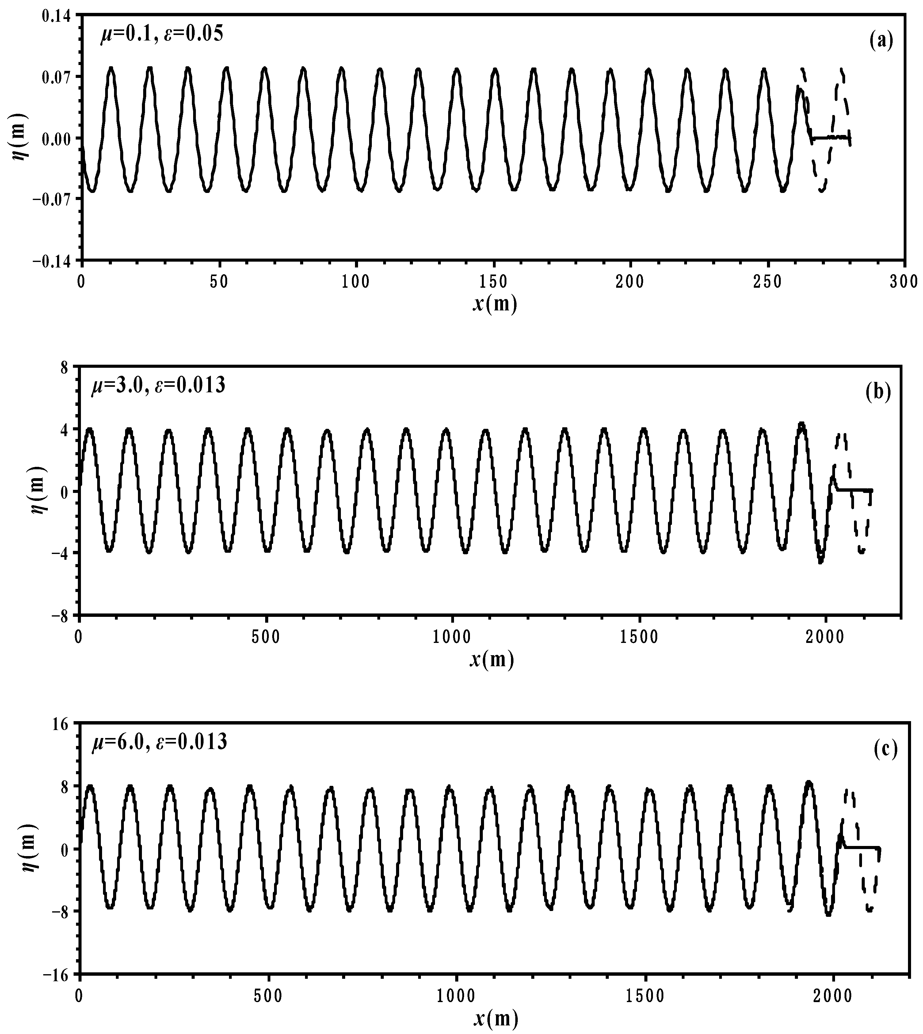
4.1. Numerical Simulation of Monochromatic Wave Propagation

As shown in Figure 1, the length of the wave flume was set at 20 times the incident wavelength. The parameters of the incident wave for the cases are listed in

Table 1. Parameters of the incident monochromatic waves.

Cases	h (m)	A (m)	H0 (m)	μ	ε	H0/h	H0/L	T (s)	L (m)
Ⅰ	1.4	0.07	0.14	0.1	0.05	0.1	0.01	4.0	14.0
II	318.0	4.0	8.0	3.0	0.013	0.025	0.075	8.24	106.0
III	636.0	8.0	16.0	6.0	0.013	0.025	0.151	12.978	106.0

. A, H₀, T, and L denote the wave amplitude, wave height, wave period, and wavelength, respectively. μ and ε denote the ratio of water depth to wavelength and the ratio of wave amplitude to water depth, respectively. $∆x$ was set as $L/50$ and $∆t$ as $T/1000$ for Case I; $∆x$ was set as $L/500$ and $∆t$ as $T/\mathrm{10,000}$ for Case II; $∆x$ was set as $L/300$ and $∆t$ as $T/\mathrm{10,000}$ for Case III.

The numerical instantaneous free surface elevations along the wave flume are compared to the theoretical ones in Figure 2. Case Ⅰ considers the transition water wave. Cases II and III consider deepwater waves. As shown in Figure 2, the wave surfaces along the wave flume are a typical regular sinusoidal waveform, which propagates uniformly and stably. The numerical results are consistent with the theoretical solutions. Therefore, compared to the conventional Boussinesq-type numerical model, the present numerical model significantly expands the applicable range of water depth and can effectively simulate wave propagation in large water depths.

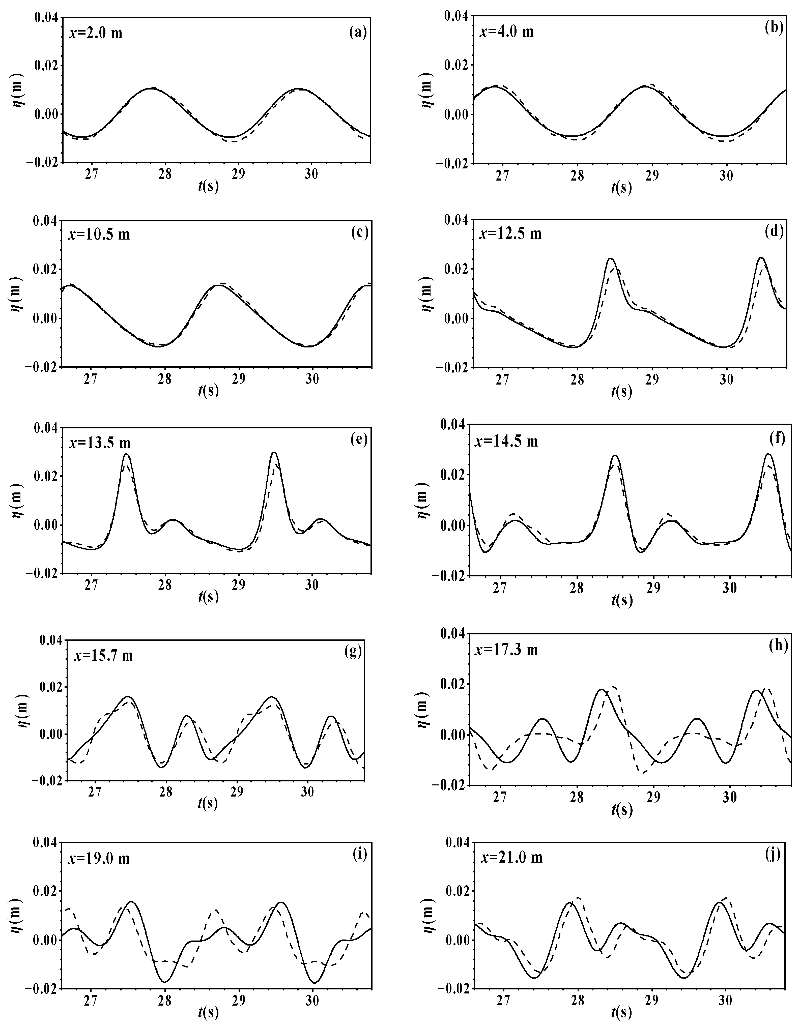
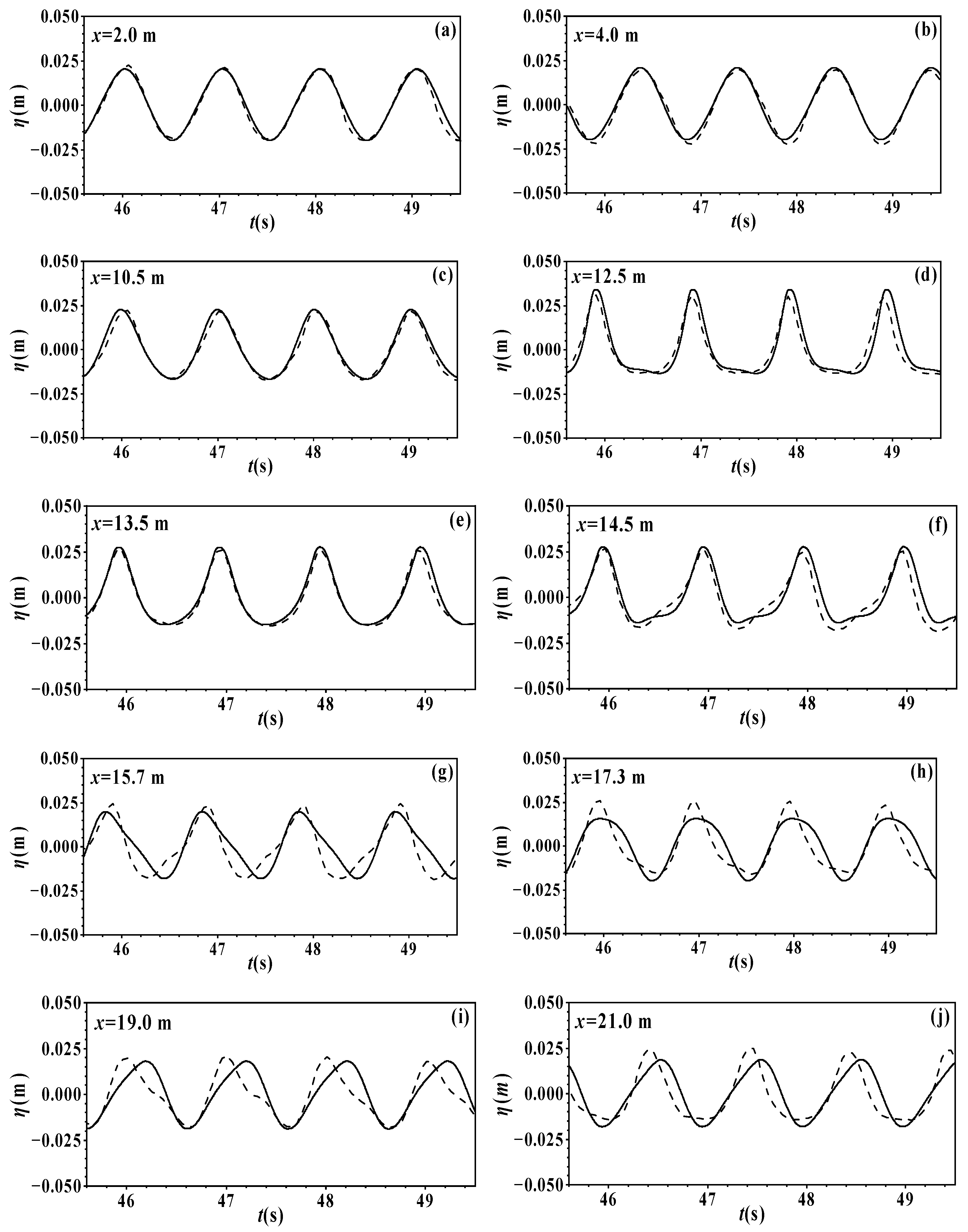
4.2. Numerical Simulation of Bichromatic Wave Propagation

To systematically simulate the propagation of bichromatic waves, four groups of bichromatic wave combinations were selected as the incident waves. The cases selected contain three types of bichromatic wave combinations: the combination of two shallow water waves, two transition water waves, and two deep water waves. The still depths for Cases A and B1 were set at 1.0 and 0.45 m, respectively. The still depths for Cases B2 and C were both set at 0.4 m. The total lengths of the numerical flume were set at 20 times the wavelength of incident wave 1 for all of the considered cases. The wave incident condition was specified by the second-order solution proposed by Hong (1980) [38], and naturally, the theoretical solutions are calculated based on Hong (1980) [38]. The parameters of the incident waves are listed in

Table 2. Parameters for different combinations of bichromatic waves.

Cases	Incident Wave 1				Incident Wave 2
	${\mathit{T}}_1\left(\mathbf{s}\right)$	${\mathit{A}}_1\left(\mathbf{m}\right)$	${\mathit{L}}_1\left(\mathbf{m}\right)$	${\mathit{\mu }}_1$	${\mathit{T}}_2\left(\mathbf{s}\right)$	${\mathit{A}}_2\left(\mathbf{m}\right)$	${\mathit{L}}_2\left(\mathbf{m}\right)$	${\mathit{\mu }}_2$
A	7.0	0.02	21.62	0.046	14.0	0.002	43.70	0.023
B1	2.0	0.01	3.88	0.12	2.5	0.01	5.0	0.09
B2	1.02	0.02	1.51	0.265	2.15	0.02	4.01	0.1
C	0.6	0.004	0.56	0.71	0.6	0.003	0.56	0.71

. $∆x$ was set at $L_1/50$ and $∆t$ at $T_1/1000$. After model tests, the wave number in the governing Equations (27) and (28) for all cases was finally set as (k₁ + k₂)/2.

Figure 3 shows the comparisons for all cases between the numerical instantaneous spatial free surface elevation and the theoretical solutions. Figure 4 shows the comparisons between the calculated time series of surface elevation and the theoretical solutions for all cases. For Case A, the amplitude of incident wave 1 is 10 times that of incident wave 2, whereas the period of incident wave 2 is 2 times that of incident wave 1. As shown in Figure 3a and Figure 4a,b, the high- and low-wave crests formed after the superposition of two waves, which becomes significant with the increase in propagation distance. The numerical solutions can more effectively illustrate the nonlinear effect than the theoretical solutions. Cases B1 and B2 consider the bichromatic wave combination of two transition water waves. The wave heights for every case are the same, and the wave groups are fully modulated wave groups. As shown in Figure 3b and Figure 4c,d, the wave group waveform changes periodically and stably, and the numerical solutions are consistent with the theoretical solutions. Comparing Figure 3b,c, and Figure 4c–f, it can be established that the second-order wave peaks appear for Case B2, which indicates that the wave-wave nonlinear interaction for Case B2 is more significant than that for Case B1. As shown in Figure 4e,f, in Case B2, there are phase differences between the numerical solutions and the theoretical solutions, and the phase difference increases as the wave propagates forward. Case C considers the bichromatic wave combination of two deepwater waves. The wave heights of the two incident waves are close, and the wave period and wavelength are the same. As shown in Figure 3d and Figure 4g,h, after the interaction of two waves with the same frequency, a regular sinusoidal waveform is still maintained; only the amplitude is the superposition of those of two single waves. Therefore, the results indicate that the present numerical model can effectively simulate the propagation and transformation of a bichromatic wave in waters of uniform water depth in most cases, except for the phase differences encountered in a particular case.

5. Numerical Simulation in the Wave Flume with an Uneven Bottom

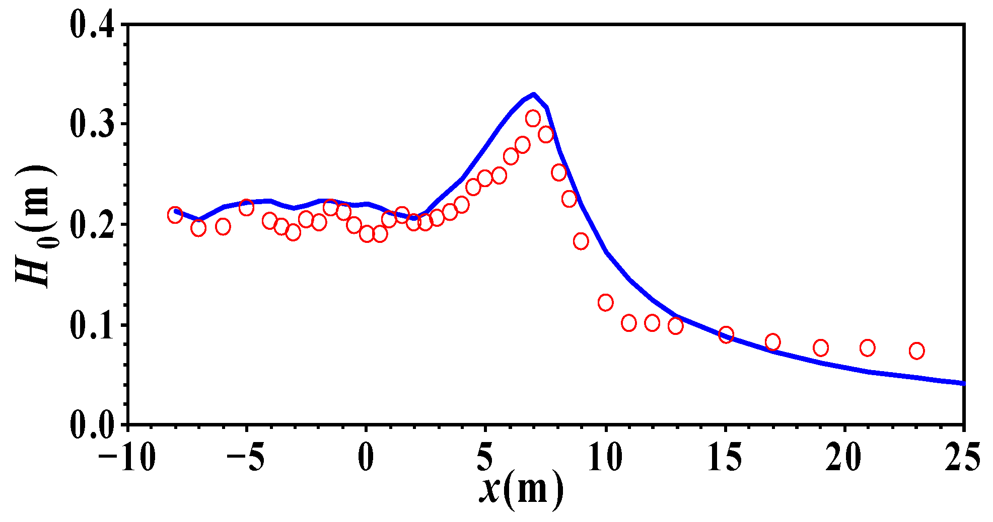
5.1. Wave Propagation over a Submerged Bar

The laboratory experiment containing a submerged bar was conducted to verify the accuracy of the numerical models based on the Boussinesq-type equations. Luth et al. (1994) [41] conducted a physical model experiment in a wave flume. The layout of the experimental set-up, the locations of the measurement stations, and the geometry of the flume are illustrated in Figure 5. The total length of the wave flume was 32.0 m. The still depth was 0.4 m in the deep region and decreased to 0.1 m at the top of the bar, which consisted of an upward slope of 1:20 and a 2.0 m horizontal crest followed by a downward slope of 1:10. Two sets of data collected by Luth et al. (1994) [41] are summarized in

Table 3. Parameters of incident waves for two cases.

Cases	I	II
H0 (m)	0.02	0.041
T (s)	2.02	1.01
μ	0.107	0.269
ε	0.025	0.051

. The incident wave boundary condition is specified with the Stokes first-order solution in this study. ∆x were selected as L/150 and L/50 for Cases I and II, respectively, and ∆t was set as T/1000 for the two cases.

Figure 6 and Figure 7 show the time series of the surface displacements at different locations for Cases I and II, respectively. As shown in Figure 6 and Figure 7, the wave shapes are less affected by the topography; that is, the wave surfaces at x = 2.0 and 4.0 m maintain a regular sinusoidal waveform. This is because the front part of the bar has a horizontal bottom. When x = 10.5 m, the wave has encountered the submerged bar; thus, the ratio of wave height to water depth is increased, nonlinear effects become significant, and the wave crests increase. Moreover, the wave profile begins to tilt in Figure 6 because the relative water depth is shallower in Case I. When x = 12.5 and 13.5 m, the wave has reached the top of the submerged bar; the wave crest becomes steeper and the wave trough becomes flatter. It can be observed from Figure 6f,g that a significant secondary wave crest occurs owing to the wave passing over the top of the submerged bar. During waves propagating from x = 14.5 to 15.7 m, the secondary wave crest increases while the primary wave crest decreases, and the phenomenon of harmonic decomposition becomes significant. As shown in Figure 6h,j, at gauges 17.3, 19.0, and 21.0 m, the waves have propagated into the deep-water region, where the secondary wave crest keeps growing. Comparing Case I to Case II, Case II has a larger relative water depth. Therefore, Case II has stronger dispersive characteristics than Case I. As shown in Figure 6 and Figure 7, the numerical results at the leading side and the top of the submerged bar are consistent with the experimental data. After the wave propagates through the submerged bar into the deep-water region, the higher harmonics are released, specifically for Case I. However, the numerical results cannot fully illustrate the existence of the released higher harmonics, which is more obvious in Figure 6 than in Figure 7. This is because the governing equations adopted in this study are weakly nonlinear, and the relative water depth for Case I is smaller than for Case II.

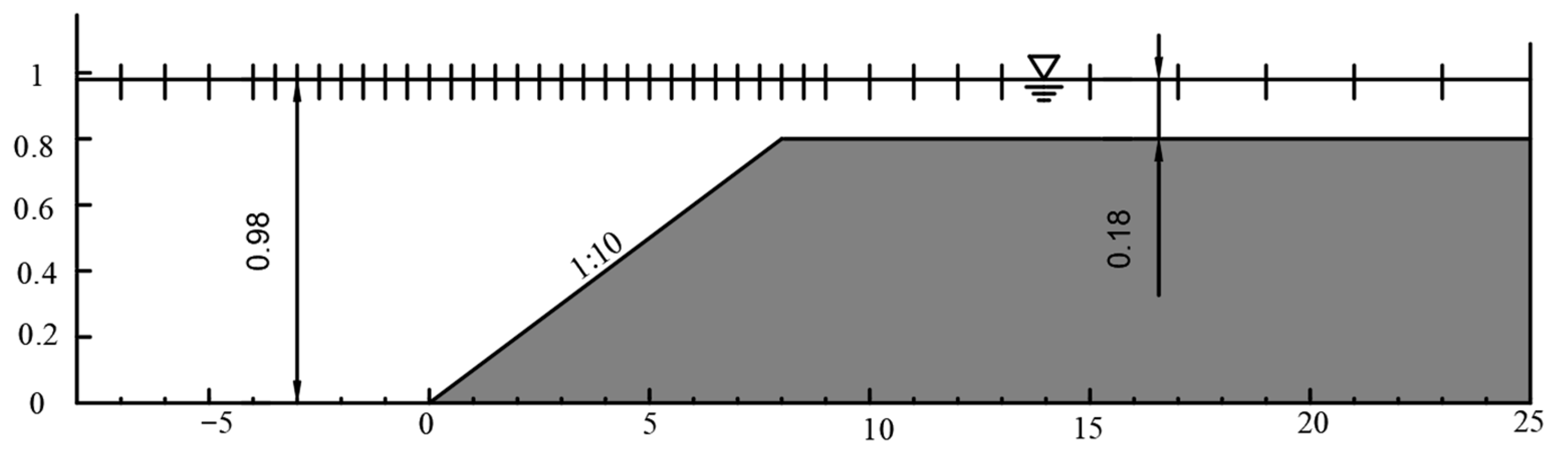
5.2. Numerical Simulation of Wave Propagation on Slopes

Tsai et al. (2005) [42] conducted three sets of physical model experiments that contain three bottom slopes of 1:10, 1:5, and 1:3 to verify empirical formulas for the breaking wave heights. The experimental parameters of the bottom slope of 1:10 were selected for numerical simulation, and the horizontal section was rough in this study.

The sketch of the experimental setup is shown in Figure 8. The horizontal ordinate denotes the distance from the toe of the slope. The still water depth is 0.98 m before the slope and decreases to 0.18 m at the top of the slope. Various wave gauges were used to measure the wave profiles, and an A–D converter at a sampling frequency of 20 Hz digitized all records. Parameters H₀, T, and L of the incident wave were selected as 0.213 m, 2.6 s, and 7.27 m, respectively. According to Kennedy et al. (2000), ${\alpha }_1$, ${\alpha }_2$, and ${\alpha }_3$ were selected as 8.0, 0.65, and 0.08, respectively. n was selected as 0.01. ∆x was set as L/60, and ∆t was set as T/1000. The total calculation time was 60 wave periods, and the time series of surface elevation during the final 5 wave periods was used for the time average wave height estimation at each grid point.

Figure 9 shows the comparison between the calculated averaged wave heights and experiment data along the wave flume. It can be established that the present numerical results are consistent with the experiment data. The averaged wave heights remain unchanged in front of the slope. When the wave travels forward and encounters the slope, the wave heights increase owing to the sharp change in water depth; finally, wave breaking occurs after the rapid increase in wave heights owing to the limitation of water depth at the top of the slope. After the wave breaking occurs, the wave height decreases rapidly within a short propagation distance. As shown in Figure 9, the present numerical model can effectively simulate the distribution of wave heights before and after wave breaking in the waters with a slope topography and can accurately capture the location of wave breaking.

6. Conclusions

In this study, a numerical model valid for wave propagation from deep to shallow water was proposed. In the numerical model, the non-conservative nonlinear equations derived by Li (2010) were first reorganized as the conservative equations and then employed as the governing equations. To solve the imbalance problem, the surface gradient term was split into an artificial flux gradient and a source term that is almost not affected by the bed slope in a non-uniform bed. The eddy viscosity-type breaking and bottom friction terms were added to the momentum equations to numerically simulate the wave-breaking phenomenon. This is because the model proposed by Li (2010) cannot numerically simulate the wave-breaking phenomenon. When the governing equations were discretized, the predictor-corrector scheme was utilized for the time integration, and a hybrid FDM and FVM scheme was employed to discretize the spatial derivatives, where the numerical flux terms were calculated by the MUSCL-TVD scheme up to the fourth-order accuracy with the Riemann solver and the spatial derivatives in the source term were discretized by FDM.

The wave propagation in water flumes with uniform depth and various topographies was simulated using the present numerical model. The calculation results indicate that the present numerical model can simulate the wave propagation in the deep waters and effectively simulate the different bichromatic wave combinations of two shallow water waves, two transition water waves, and two deep water waves. The numerical results of the wave propagation over a bar and a sloped beach were compared to the experiment data. It is shown that the present numerical model can simulate the wave shoaling and nonlinearity over a bar and accurately predict the position of the breaking point, and that the calculated wave heights are consistent with the experiment data.

The one-dimensional numerical model proposed in this study will be extended to a two-dimensional model in the near future.

References

1. Peregrine, D.H. Long waves on a beach. J. Fluid Mech. 1967, 27, 815–827. [Google Scholar] [CrossRef]
2. Madsen, P.A.; Murray, R.; Sørensen, O.R. A new form of the Boussinesq equations with improved linear dispersion characteristics. Coast. Eng. 1991, 15, 371–388. [Google Scholar] [CrossRef]
3. Nwogu, O. Alternative form of Boussinesq equations for nearshore wave propagation. J. Waterw. Port Coast. Ocean Eng. 1993, 119, 618–638. [Google Scholar] [CrossRef]
4. Wei, G.; Kirby, J.T.; Grilli, S.T.; Subramanya, R. A fully nonlinear Boussinesq model for surface waves. Part 1. Highly nonlinear unsteady waves. J. Fluid Mech. 1995, 294, 71–92. [Google Scholar] [CrossRef]
5. Hong, G.W. High order models of nonlinear and dispersive wave in water of varying depth with arbitrary slopping bottom. China Ocean Eng. 1997, 11, 243–260. [Google Scholar]
6. Zhang, H.S.; Zhou, H.W.; Hong, G.W. A set of high order nonlinear Boussinesq-type equations and its numerical verification. Chin. J. Hydrodyn. Ser. A 2011, 26, 265–277. (In Chinese) [Google Scholar]
7. Berkhoff, J.C.W. Computation of combined refraction-diffraction. In Proceedings of the 13th Confference on Coastal Engineering, Vancouver, BC, Canada, 10–14 July 1972; pp. 471–490. [Google Scholar]
8. Hong, G.W. Mathematical models for combined refraction-diffraction of waves on non-uniform current and depth. China Ocean Eng. 1996, 10, 433–454. [Google Scholar]
9. Panchang, V.G.; Wei, G.; Pearce, B.R.; Briggs, M.J. Numerical simulation of irregular wave propagation over shoal. J. Waterw. Port Coast. Ocean Eng. 1990, 116, 324–340. [Google Scholar] [CrossRef]
10. Kirby, J.T.; Dalrymple, R.A. An approximate model for nonlinear dispersion in monochromatic wave propagation models. Coast. Eng. 1986, 9, 545–561. [Google Scholar] [CrossRef]
11. Tsai, C.P.; Chen, H.B.; Hsu, J.R.C. Second-order time-dependent mild-slope equation for wave transformation. Math. Probl. Eng. 2014, 2014, 341385. [Google Scholar] [CrossRef]
12. Kim, I.C.; Kaihatu, J.M. A consistent nonlinear mild-slope equation model. Coast. Eng. 2021, 170, 104006. [Google Scholar] [CrossRef] [PubMed]
13. Tang, Y.; Ouellet, Y. A new kind of nonlinear mild-slope equation for combined refraction-diffraction of multifrequency waves. Coast. Eng. 1997, 31, 3–36. [Google Scholar] [CrossRef]
14. Wu, Z.; Hong, G.W.; Zhang, H.S.; Zhang, Y. Numerical model and application of fully dispersive nonlinear wave. In Proceedings of the 14th China Marine (Shore) Engineering Symposium, Hohhot, China, 5 August 2009; pp. 460–469. (In Chinese). [Google Scholar]
15. Li, B. Wave equations for regular and irregular water wave propagation. J. Waterw. Port Coast. Ocean Eng. 2008, 134, 121–142. [Google Scholar] [CrossRef]
16. Li, B. A mathematical model for weakly nonlinear water wave propagation. Wave Motion 2010, 47, 265–278. [Google Scholar] [CrossRef]
17. Hong, G.W.; Zhang, H.S.; Feng, W.B. Numerical simulation of nonlinear three-dimensional waves in water of arbitrary varying topography. China Ocean. Eng. 1998, 12, 383–404. [Google Scholar]
18. Zhang, H.S.; Zhao, H.J.; Ding, P.X.; Miao, G.P. On the modeling of wave propagation on non-uniform currents and depth. Ocean Eng. 2007, 34, 1393–1404. [Google Scholar] [CrossRef]
19. Fang, K.Z.; Zou, Z.L. Boussinesq-type equations for nonlinear evolution of wave trains. Wave Motion 2010, 47, 12–32. [Google Scholar] [CrossRef]
20. Zhao, M.; Teng, B.; Cheng, L. A new form of generalized Boussinesq equations for varying water depth. Ocean Eng. 2004, 31, 2047–2072. [Google Scholar] [CrossRef]
21. Liu, S.; Sun, Z.; Li, J. An unstructured FEM model based on Boussinesq equations and its application to the calculation of multidirectional wave run-up in a cylinder group. Appl. Math. Model. 2012, 36, 4146–4164. [Google Scholar] [CrossRef]
22. Kirby, J.T.; Wei, G.; Chen, Q.; Kennedy, A.B.; Dalrymple, R.A. FUNWAVE 1.0: Fully Nonlinear Boussinesq Wave Model-Documentation and User’s Manual; Research Report NO. CACR-98-06; University of Delaware: Newark, NJ, USA, 1998. [Google Scholar]
23. Walkley, M.; Berzins, M. A finite element method for the two-dimensional extended Boussinesq equations. Int. J. Numer. Methods Fluids 2002, 39, 865–885. [Google Scholar] [CrossRef]
24. Erduran, K.S.; Ilic, S.; Kutija, V. Hybrid finite-volume finite-difference scheme for the solution of Boussinesq equations. Int. J. Numer. Methods Fluids 2005, 49, 1213–1232. [Google Scholar] [CrossRef]
25. Madsen, P.A.; Sørensen, O.R. A new form of the Boussinesq equations with improved linear dispersion characteristics. Part 2. A slowly-varying bathymetry. Coast. Eng. 1992, 18, 183–204. [Google Scholar] [CrossRef]
26. Yamamoto, S.; Daiguji, H. Higher-order-accurate upwind schemes for solving the compressible Euler and Navier-Stokes equations. Comput. Fluids 1993, 22, 259–270. [Google Scholar] [CrossRef]
27. Frazão, S.S.; Zech, Y. Undular bores and secondary waves-experiments and hybrid finite-volume modelling. J. Hydraul. Res. 2002, 40, 33–43. [Google Scholar] [CrossRef]
28. Tonelli, M.; Petti, M. Hybrid finite volume-finite difference scheme for 2DH improved Boussinesq equations. Coast. Eng. 2009, 56, 609–620. [Google Scholar] [CrossRef]
29. Roeber, V.; Cheung, K.F.; Kobayashi, M.H. Shock-capturing Boussinesq-type model for nearshore wave processes. Coast. Eng. 2010, 57, 407–423. [Google Scholar] [CrossRef]
30. Shi, F.Y.; Kirby, J.T.; Harris, J.C.; Geiman, J.D.; Grilli, S.T. A high-order adaptive time-stepping TVD solver for Boussinesq modeling of breaking waves and coastal inundation. Ocean Model. 2012, 43, 36–51. [Google Scholar] [CrossRef]
31. Choi, Y.K.; Shi, F.Y.; Malej, M.; Smith, J.M. Performance of various shock-capturing-type reconstruction schemes in the Boussinesq wave model, FUNWAVE-TVD. Ocean Model. 2018, 131, 86–100. [Google Scholar] [CrossRef]
32. Kennedy, A.B.; Chen, Q.; Kirby, J.T.; Dalrymple, R.A. Boussinesq modeling of wave transformation, breaking, and runup. I: 1D. J. Waterw. Port Coast. Ocean Eng. 2000, 126, 39–47. [Google Scholar] [CrossRef]
33. Kim, D.H.; Lynett, P.J.; Socolofsky, S.A. A depth-integrated model for weakly dispersive, turbulent, and rotational fluid flows. Ocean Model. 2009, 27, 198–214. [Google Scholar] [CrossRef]
34. Yao, Y.; Huang, Z.H.; Monismith, S.G.; Lo, E.Y.M. 1DH Boussinesq modeling of wave transformation over fringing reefs. Ocean Eng. 2012, 47, 30–42. [Google Scholar] [CrossRef]
35. Zhao, D.H.; Shen, H.W.; Lai, J.S.; Tabios, G.Q., III. Approximate Riemann solvers in FVM for 2D hydraulic shock wave modeling. J. Hydraul. Eng. 1996, 122, 692–702. [Google Scholar] [CrossRef]
36. Rogers, B.; Fujihara, M.; Borthwick, A.G.L. Adaptive Q-tree Godunov-type scheme for shallow water equations. Int. J. Numer. Methods Fluids 2001, 35, 247–280. [Google Scholar] [CrossRef]
37. Rogers, B.D.; Borthwick, A.G.L.; Taylor, P.H. Mathematical balancing of flux gradient and source terms prior to using Roe’s approximate Riemann solver. J. Comput. Phys. 2003, 192, 422–451. [Google Scholar] [CrossRef]
38. Hong, G.W. On the nonlinear interactions among gravity surface waves. Acta Oceanol. 1980, 2, 158–180. (In Chinese) [Google Scholar]
39. Shiach, J.B.; Mingham, C.G. A temporally second-order accurate Godunov-type scheme for solving the extended Boussinesq equations. Coast. Eng. 2009, 56, 32–45. [Google Scholar] [CrossRef]
40. Larsen, J.; Dancy, H. Open boundaries in short wave simulations—A new approach. Coast. Eng. 1983, 7, 285–297. [Google Scholar] [CrossRef]
41. Luth, H.R.; Klopman, G.; Kitou, N. Kinematics of Waves Breaking Partially on an Offshore Bar: LDV Measurements of Waves with and without a Net Onshore Current; Report H-1573, Delft Hydraulics; IOP Publishing Ltd.: Delft, The Netherlands, 1994; Volume 40. [Google Scholar]
42. Tsai, C.P.; Chen, H.B.; Hwung, H.H.; Huang, M.J. Examination of empirical formulas for wave shoaling and breaking on steep slopes. Ocean Eng. 2005, 3, 469–483. [Google Scholar] [CrossRef]
Figure 1. Sketch of the numerical wave flume.
Jmse 11 01003 g001
Figure 2. Comparisons of the instantaneous wave profiles for monochromatic waves (dashed line: theoretical solutions; solid line: numerical solutions) [(a) μ = 0.1, ε = 0.05; (b) μ = 3.0, ε = 0.013; (c) μ = 6.0, ε = 0.013].
Jmse 11 01003 g002
Figure 3. Comparisons of the instantaneous wave profiles for bichromatic waves (dashed line: theoretical solutions; solid line: numerical solutions) [(a) Case A; (b) Case B1; (c) Case B2; (d) Case C].
Jmse 11 01003 g003
Figure 4. Comparisons of the time series of surface displacement at different locations for bichromatic waves (dashed line: theoretical solutions; solid line: numerical solutions) [(a) Case A, x = 5.0 L 1 ; (b) Case A, x = 15.0 L 1 ; (c) Case B1, x = 5.0 L 1 ; (d) Case B1, x = 15.0 L 1 ; (e) Case B2, x = 5.0 L 1 ; (f) Case B2, x = 15.0 L 1 ; (g) Case C, x = 5.0 L 1 ; (h) Case C, x = 15.0 L 1 ].
Jmse 11 01003 g004
Figure 5. Sketch of a wave flume with a submerged bar following the experimental setup by Luth et al. (1994) (m) [41].
Jmse 11 01003 g005
Figure 6. Comparisons of the time series of surface displacement at different locations for Case I (dashed line: experimental data; solid line: numerical solutions) [(a) x = 2.0 m; (b) x = 4.0 m; (c) x = 10.5 m; (d) x = 12.5 m; (e) x = 13.5 m; (f) x = 14.5 m; (g) x = 15.7 m; (h) x = 17.3 m; (i) x = 19.0 m; (j) x = 21.0 m].
Jmse 11 01003 g006
Figure 7. Comparisons of the time series of surface displacement at different locations for Case II (dashed line: experimental data; solid line: numerical solutions) [(a) x = 2.0 m; (b) x = 4.0 m; (c) x = 10.5 m; (d) x = 12.5 m; (e) x = 13.5 m; (f) x = 14.5 m; (g) x = 15.7 m; (h) x = 17.3 m; (i) x = 19.0 m; (j) x = 21.0 m].
Jmse 11 01003 g007
Figure 8. Sketch of a wave flume following the experimental setup by Tsai et al. (2005) [42].
Jmse 11 01003 g008
Figure 9. Comparisons of the time average wave heights along the wave flume (red circle: experiment data; solid line: numerical solutions).
Jmse 11 01003 g009