Assessing the Reliability of a New One-Line Model for Predicting Shoreline Evolution with Impoundment Field Experiment Data

Abstract

The advancement of knowledge in the field of coastal morphodynamics is currently highly relevant, as it provides valuable insights into the complex and dynamic nature of coastal systems and helps coastal engineers and researchers to better understand and manage the risks associated with coastal hazards. Managing and protecting coastal areas requires accurate measurements and the availability of reliable numerical models for predicting shoreline evolution. The present study focuses on verifying the reliability of a recent one-line model: the General Shoreline beach (GSb) model. The numerical simulations were performed using wave data observed by the Acoustic Wave and Current profiler and the Channel Coast Observatory buoy. The numerical results were compared with high-resolution shoreline data collected from an ARGUS monitoring station during the impoundment experiment conducted in Milford-on-Sea, UK. The numerical results demonstrated that the GSb model accurately predicts shoreline evolution, particularly for mixed beaches. The findings of the present study also show the effectiveness of the GSb online numerical model in predicting day-to-day changes in shoreline dynamics caused by wave attack. The high-resolution dataset of the ARGUS observations combined with wave data collected during the field experiment could be valuable resources for coastal researchers to further evaluate and improve numerical models of coastal morphodynamics.

1. Introduction

The coastal zone is a popular and growing area of interest due to its social, political, and economic significance. However, rapid development and use of the coastal zone have resulted in adverse effects on beach equilibrium, leading to severe erosion and, sometimes, beach disappearance. The coastal environment is highly susceptible to the impacts of climate change and sea-level rise [1].

The effective management and protection of coastal areas require reliable measurements and predictions of shoreline evolution. This information is essential for making informed coastal management decisions, such as land-use planning, coastal protection design, and adaptation to sea-level rise. Therefore, there is a need for robust and accurate methods to study coastal morphodynamics [2,3].

Various methods exist for studying coastal morphodynamics, including remote sensing techniques, field measurements, and physical and numerical models [4,5,6,7,8,9,10]. Over several decades, researchers and engineers inspired by coastal sediment processes have conducted field and laboratory experiments to learn more about coastal and sediment dynamics. Understanding the physical processes governing the morphodynamics and the rapid advance in computation technology have increased the interest in developing numerical models. Sophisticated models, such as Delft3D, have been developed to reproduce coastal morphodynamics [11,12]. These models are highly detailed and can accurately simulate complex physical processes, but their computational requirements can make them impractical for certain applications (e.g., long-term simulations). Given the complexity of the processes, which cannot be fully represented by deterministic formulas, and the high uncertainty in wave and sediment transport data [13], numerous runs are necessary for sensitivity analysis and model calibration, making the practical use of such sophisticated models prohibitive [14].

In this context, one-line models have demonstrated practical capability in predicting shoreline evolution and assisting in the selection of the most appropriate protection design in the planning of projects located in the nearshore zone [15].

However, their utility is often limited by the lack of a universal one-line model that can estimate shoreline change for various types of coastal mounds, such as sandy, gravel, cobble, and mixed beaches. Furthermore, the most common one-line models [6,7,8,9] are more difficult to calibrate due to the presence of two calibration coefficients; in fact, for a model with two calibration coefficients, initial values are chosen and simulations are run to match observed data through iterative parameter adjustments until the pair of calibration parameters that minimizes the difference between observed and calculated shorelines is found.

This limitation highlights the need for reliable models that can account for the complex processes that govern coastal morphodynamics while maintaining practical utility. To accurately evaluate the reliability of a numerical model, it is crucial to compare its predictions with high-resolution field data.

The present paper aims to address this limitation by verifying the reliability of a recent one-line model proposed by [16,17]: the General Shoreline beach (GSb) model. The high-resolution data acquired from an ARGUS monitoring station over a 740 m domain during a field experiment conducted in Milford-on-Sea, UK, were utilized to verify the reliability of the numerical solution proposed by the GSb model. The field experiment focused on the impoundment technique, in which a temporary impermeable groin was constructed to study the shoreline evolution and sediment transport [18,19,20]. The numerical simulations were performed using both nearshore wave data and propagated wave data from offshore (buoy location) to nearshore using the SWAN numerical model.

The numerical results have demonstrated favorable agreement, indicating that the GSb model has the potential to accurately predict the shoreline evolution in the case of mixed beaches. Furthermore, the results also showcase the effectiveness of the GSb online numerical model in forecasting the day-to-day changes in shoreline dynamics caused by wave attack.

The high-resolution dataset of the ARGUS observations and wave data acquired during the impoundment experiment, presented for the first time in the present study, represent a valuable resource for coastal researchers to further evaluate and improve numerical models of coastal morphodynamics.

2. Materials and Methods

2.1. Field Experiment

2.1.1. Study Area

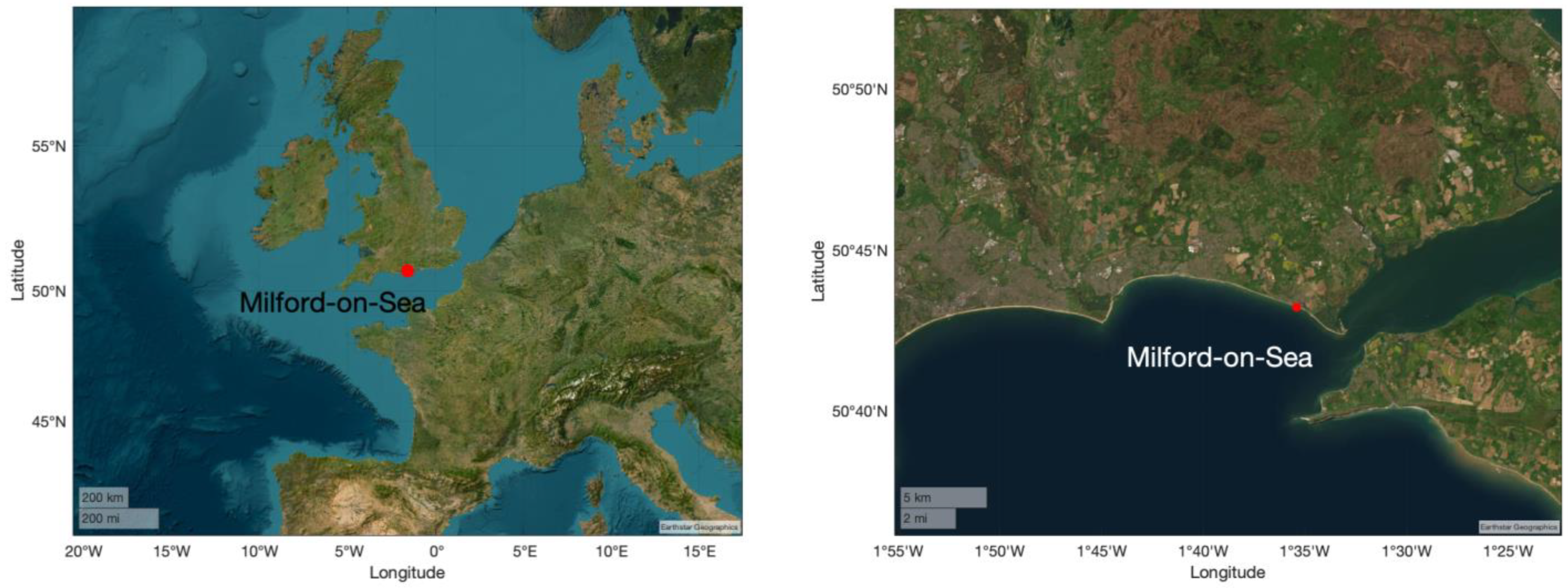
Milford-on-Sea is located at the eastern side of Christchurch Bay in Hampshire, UK, as shown in Figure 1. The area is of particular interest due to its unique coastal elements, including a cliff eroding at the western side near Barton on Sea, a natural beach at Hordle Cliff, and coastal defense structures comprising timber groins and a seawall between Milford-on-Sea and Hurst Spit. The field site is subject to predominant SSW wave direction and semi-diurnal tides with a spring tidal range of 2 m.

The area is characterized by a beach composed of finer (sand) and coarser (cobbles, gravel) sediment grains. The median grain size of the total sample composing the mixed beach, D₅₀, is equal to 11.19 mm. The relationship between D₈₅ and D₁₅ is 27.79 (where D₈₅ and D₁₅ represent the particle diameter for which 85% and 15%, respectively, of the material is finer). Figure 2 shows the percentage of material passing through the sieve for three different samples: fine, coarse, and the total sample. Three dashed red lines are also included in the graph to indicate the percentage of material passing through specific sieve sizes. The figure also displays the values of D₁₅, D₅₀, and D₈₅ for each sample, where the subscripts F, C, and T correspond to the finer, coarse, and total sample, respectively.

According to a sediment transport investigation carried out by [21], Christchurch Bay had a relatively recent geological origin. This bay was formed as a result of the shoreline retreating during the mid to late Holocene transgression that occurred during the Quaternary Period. The stretch of coast from Barton on Sea to Hurst Spit has been identified and designated as a Site of Special Scientific Interest (SSSI). Milford-on-Sea is also recognized as a Coastal Area of Outstanding Natural Beauty (AONB) by [21].

2.1.2. Impoundment Technique

Measuring longshore transport is challenging both in the field and laboratory due to the combination of suspended and bedload sediment transport. Instruments have been developed to measure suspended sediment concentrations at a point, but no satisfactory method of measuring bedload has yet been demonstrated [22]. The total longshore sediment transport rate in the surf zone can be evaluated with a method noted as “impoundment” that consists in deploying a temporary structure (i.e., groin) across the beach to capture sediment transported by waves and currents. After a given period of time, the accumulated sediment in the impoundment structure is measured and analyzed to determine the sediment transport rate along the coastline. This technique is considered, by several authors, a reliable and effective method to estimate longshore transport rates [23,24,25,26].

In 2007, a field experiment based on the impoundment technique was performed at the study site, deploying a temporary impermeable groin, 46 m long (originally 19 m wet and 27 m dry), which acted as a barrier to the longshore sediment transport between 1 October 2007 and 15 November 2007 (Figure 3) [18,19,20].

2.1.3. Argus Beach Monitoring System (ARGUS) Shoreline Data

The Argus Beach Monitoring System (ARGUS) is an advanced coastal monitoring system that employs a network of cameras to provide real-time monitoring of coastal zones. The system uses sophisticated algorithms to address a wide range of coastal issues, such as shoreline evolution, impact of groins, and beach nourishments. Shorelines can be automatically detected through methods that rely on identifying a bright band linked to the shore break or a color variation between wet and dry sand [27,28,29,30].

As part of RF-PeBLE project, Risk-based Framework for Predicting Long-term Beach Evolution, ARGUS was installed at the study site from January 2007 until October 2011. The system consisted of five cameras facing the beach and mounted at the top of the cliff (16 m high).

Appendix A provides a list of specific ARGUS shorelines selected to ensure consistency in tidal levels among those available during the field experiment period (from 1 October 2007 to 15 November 2007). The tidal level recorded at Becton Bunny (Barton on Sea) at the acquiring time of the selected ARGUS shorelines have also been included in Appendix A [19].

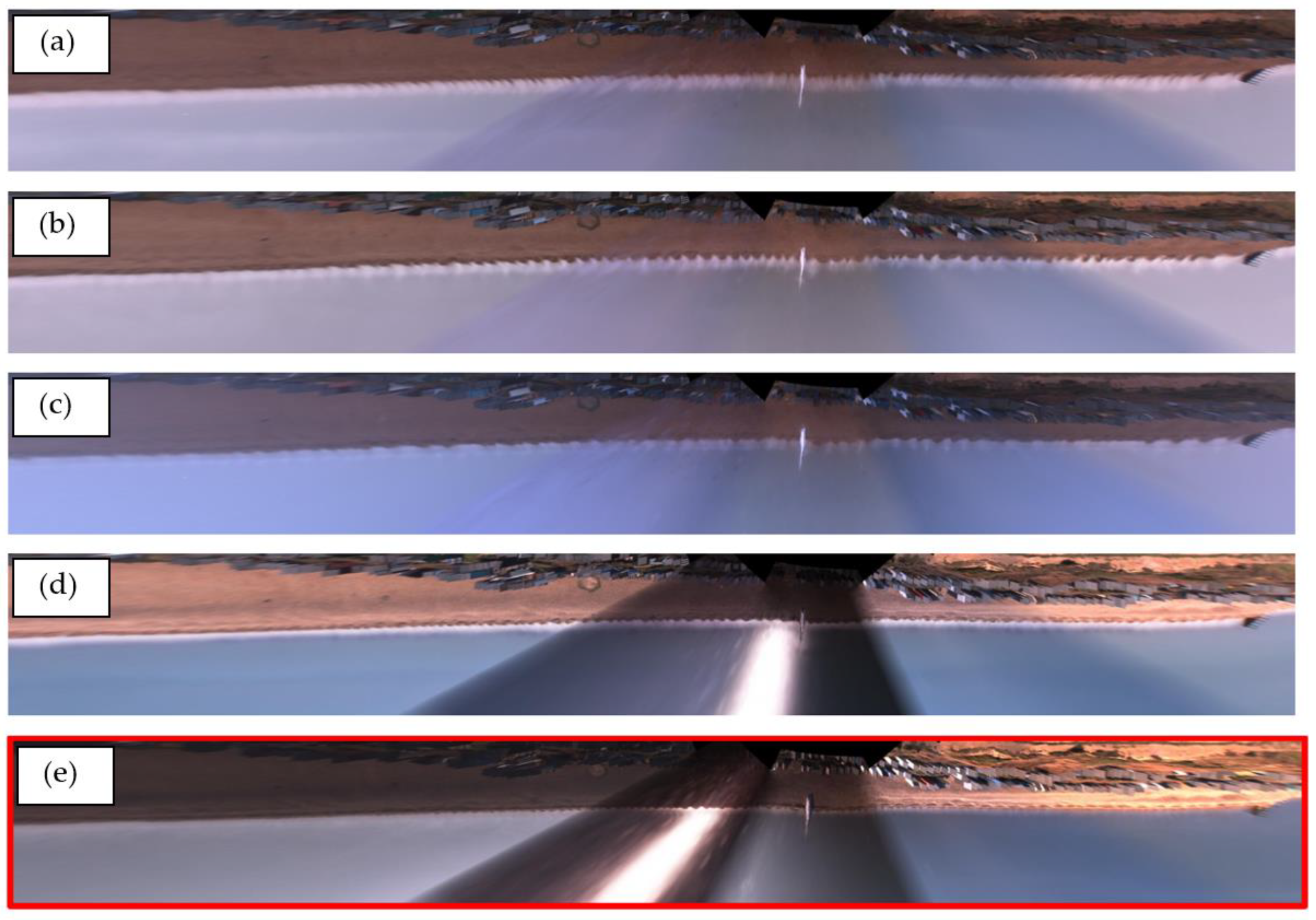
Figure 4a–e show the first 5 available ARGUS images during the field experiment period. The figures correspond to the following dates and times: (a) 1 October 2007 at 16:50, (b) 2 October 2007 at 09:30, (c) 3 October 2007 at 06:30, (d) 4 October 2007 at 13:50, and (e) 5 October 2007 at 15:50. The shoreline is not always well defined due to visible foam in breaking waves at the water–beach interface. ARGUS images are selected during a calm sea state to ensure accurate identification of the shoreline. For example, the first selected image among the first 5 available is the image taken on 5 October 2007 at 15:50 (Figure 4e), representing the first image where the shoreline is clearly detectable.

2.1.4. AWAC Wave Data

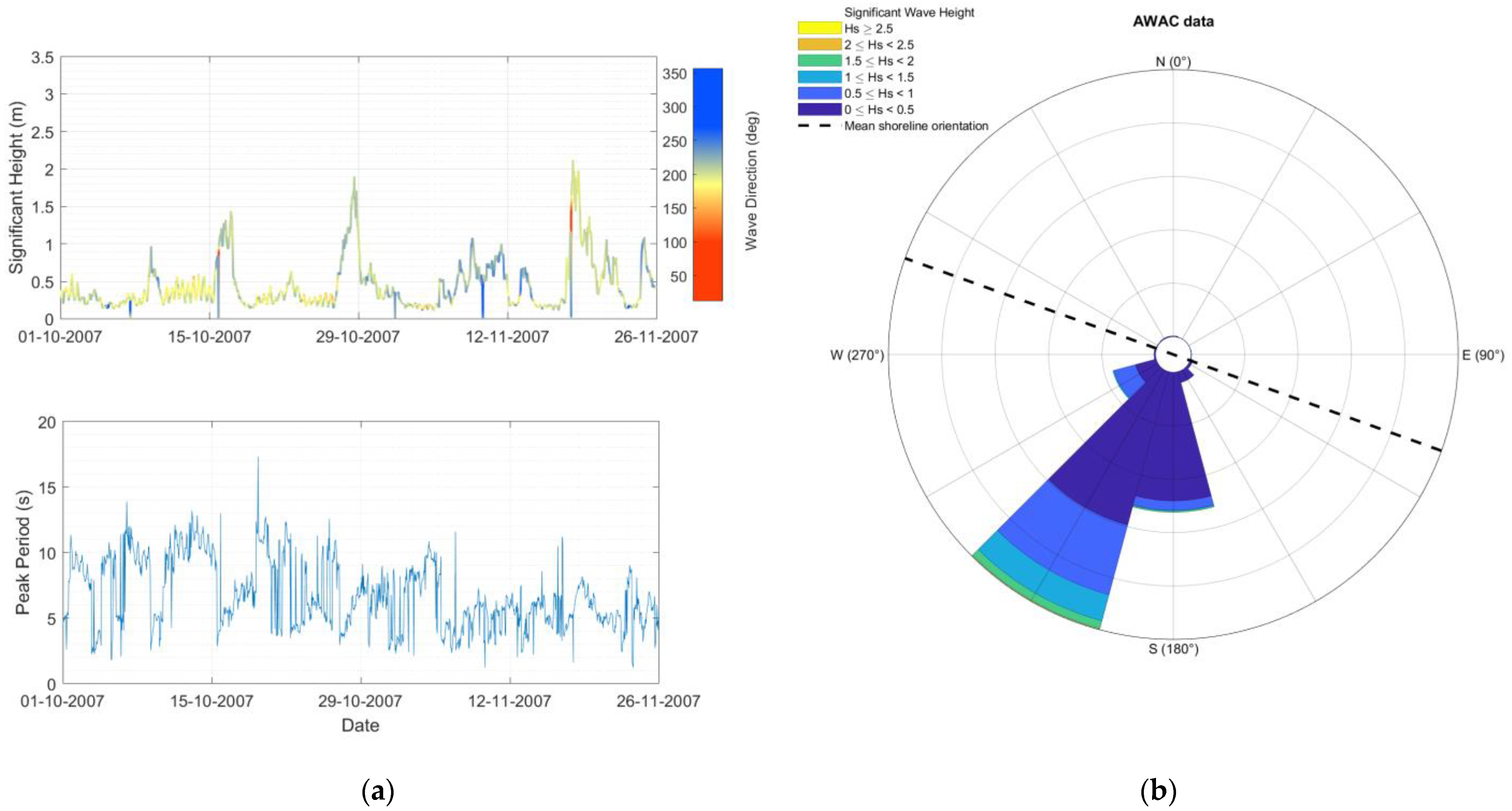
The Nortek Acoustic Wave and Current (AWAC) profiler was used to collect significant wave height, peak period, and mean wave direction with hourly time step during the period from 1 October 2007 to 25 November 2007 (Figure 5). The AWAC profiler was located at a water depth of 7 m, approximately 600 m offshore. The wave direction is referred to with respect to the geographic north. The line color of the significant wave height (up panel of Figure 5a) depends on the wave direction. The green color corresponds to waves from orthogonal direction to the mean shoreline orientation (no longshore transport). The blue color indicates waves coming from an angular sector producing a negative longshore transport (waves from SSW), whereas yellow/red colors represent waves coming from the angular sector producing a positive longshore transport (waves from SSE). In the wave rose (Figure 5b), the mean shoreline orientation is indicated by a dashed black line.

2.1.5. CCO Wave Data

The Milford Directional Waverider Buoy, which is part of the Southeast Regional Coastal Monitoring Programme, is located at a water depth of approximately 10 m, approximately 1500 m offshore from the study area. The Datawell Directional Waverider Mk III is the wave buoy model used to collect data. The dataset was developed by the Channel Coastal Observatory (CCO). The spatial reference system used is WGS84, with a planar coordinate encoding method of latitude/longitude. The resolution of the X and Y axes is 0.00001 decimal degrees. The parameters collected by the buoy are averaged over 30 min, with a sampling frequency of 3.84 Hz, and then downsampled to 1.28 Hz before calculation of wave parameters. The wave data are collected with respect to the geographic north.

Figure 6 shows significant wave height, peak period, and mean wave direction collected during the period from 1 October 2007 to 25 November 2007. The line color of the significant wave height (up panel of a) depends on the wave direction. The green color corresponds to waves from orthogonal direction to the mean shoreline orientation (no longshore transport). The blue shades indicate waves coming from an angular sector producing a negative longshore transport (waves from SSW), whereas yellow/red colors represent waves coming from the angular sector producing a positive longshore transport (waves from SSE). In the wave rose (Figure 5b), the mean shoreline orientation is indicated by a dashed black line.

2.1.6. Wave Propagation of Waverider Buoy data to AWAC Location

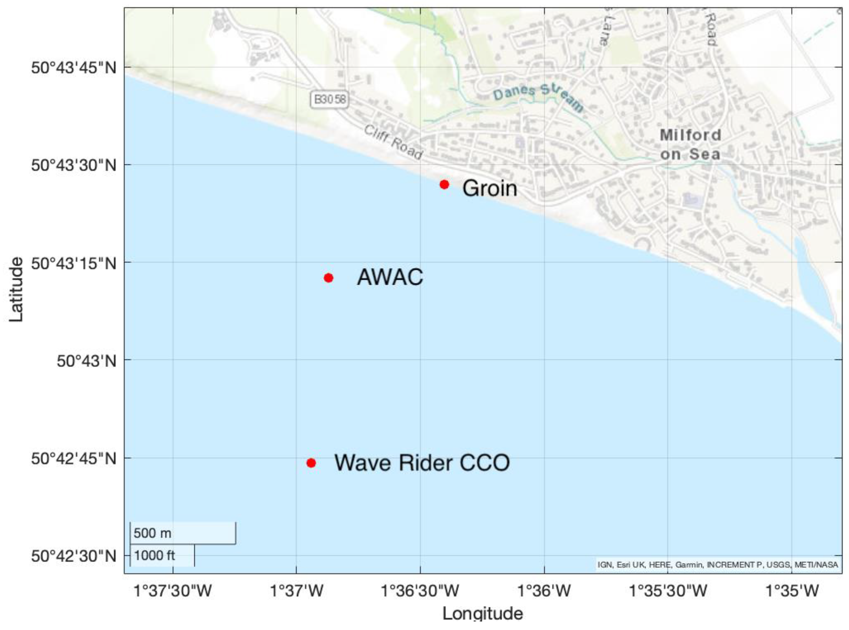
The third-generation wave model, SWAN, developed by the Delft University of Technology [31], was used to propagate the wave data collected by the Directional Waverider Buoy from its location, approximately 1500 m offshore at a water depth of 10 m (50.71229 N, −1.61568 E), to the AWAC location, approximately 600 m offshore at a water depth of 7 m (50.72015 N; −1.61450 E) (Figure 7).

The bathymetry data of Milford-on-Sea were obtained from the EMODNET portal (http://portal.emodnet-bathymetry.eu/ accessed on 17 January 2019) in ESRI ASCII format. Figure 8 shows the “Area of interest” and the corner grid point coordinates X₀, Y₀ (−1.655 E, 50.710 N).

The bathymetry data in the selected area are a matrix consisting of 23 rows and 68 columns, with a grid spacing of 73.577 m in the x-direction and 115.878 m in the y-direction. The bathymetry data grid length in the x-direction is 4929.664 m, and in the y-direction it is 2598.318 m.

Table 1. Data grid information of the EMODnet bathymetry.

Parameter	Value
n. row	23
n. columns	68
Cell size (°)	0.001041667
Cell size x (m)	73.577
Cell size y (m)	115.878
x-direction grid length (m)	4929.664
y-direction grid length (m)	2549.318
origin axis coordinate	50.710 N, −1.655 E

provides a summary of the data grid information.

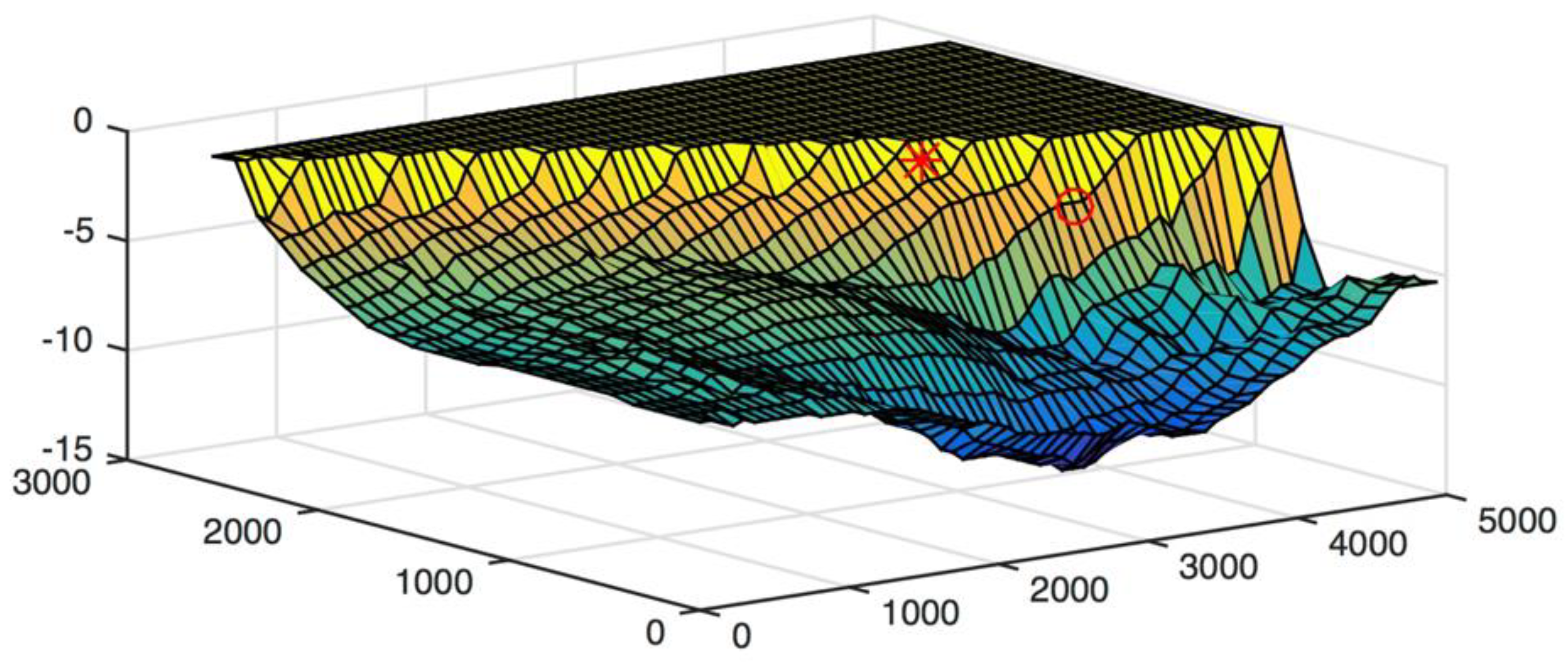
The contour map and the 3D mesh of the bathymetry are shown in Figure 9.

A uniform rectangular SWAN computational grid was defined, with the origin at the point of coordinate x_pc = 0.0 and y_pc = 0.0. The SWAN computational grid is 4929 m in length in the x-direction and 2549 m in the y-direction. The regular mesh is composed of 67 cells 73.48 m long in the x-direction and 22 cells 115.88 m long in the y-direction. The wave data collected by the Waverider Buoy (CCO) from 1 October 2007 to 25 November 2007 were used as input for the SWAN model at the south, west, and east boundaries, with the clockwise convention for wave direction.

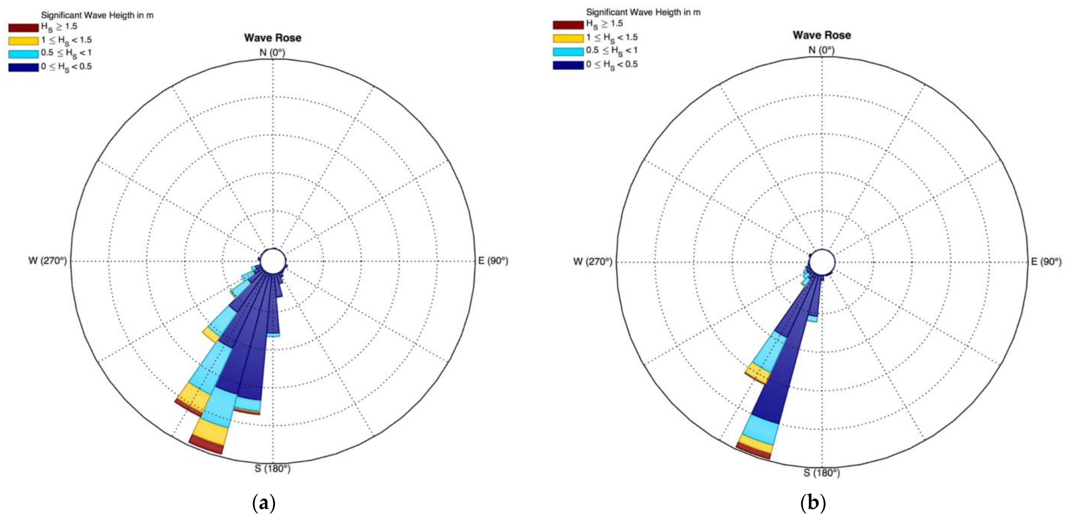
Figure 10a shows the wave rose of the AWAC data collected during the groin experiment, from 1 October 2007 to 25 November 2007 at a water depth of 7 m. Figure 10b shows the wave characteristics computed by the SWAN model at the AWAC location.

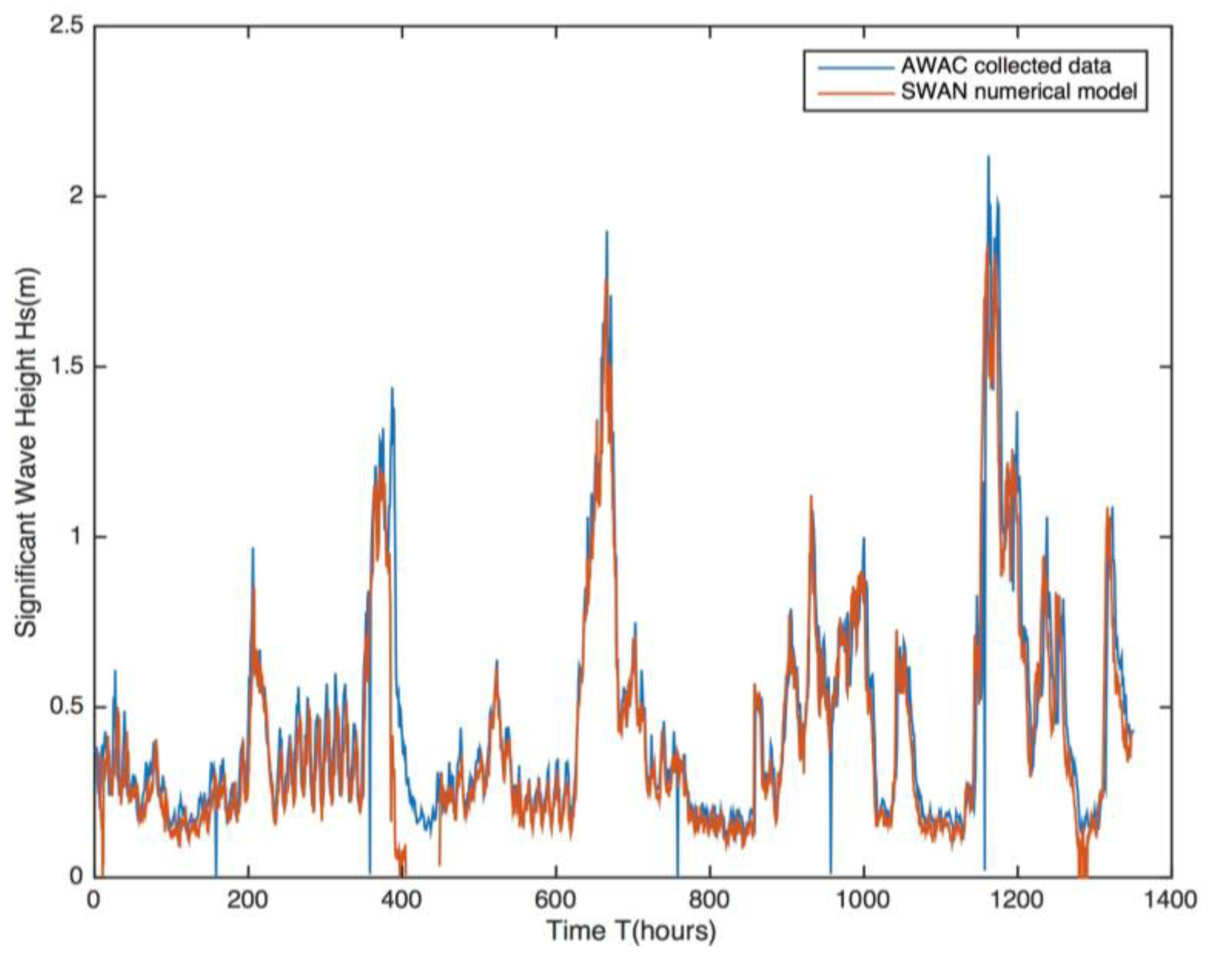
Figure 11 shows the comparison between the AWAC time series and numerical results of the significant wave height.

The results show a good agreement between the observed and computed wave parameters at the AWAC location.

2.2. Numerical Modelling of Shoreline Evolution

2.2.1. The General Shoreline Beach (GSb) Model

The General Shoreline beach (GSb) model is a morphodynamics model that belongs to the category of one-line models widely used by coastal engineers and scientists for predicting shoreline evolution. The mathematical theory of one-line models was first developed by [32], based on the assumption that (i) the cross-shore beach profile moves parallel to itself and remains constant over time, as evaluated by [33,34], and (ii) longshore sediment transport occurs within the active beach profile defined between the top of the active berm and the closure depth.

Unlike other one-line models [6,7,8,9] that rely on two calibration coefficients, K₁ and K₂, the GSb model presents a single calibration coefficient, K_GSb, which is a function of the longshore gradient in breaking wave height [35].

According to [36,37], the model is capable of predicting shoreline changes over both short-term (daily) and long-term (yearly) periods and can simulate any combination of hard structures (such as groins, detached breakwaters, and seawalls) and beach fills along a modeled coastal length.

The GSb model evaluates shoaling and refraction processes using an internal module proposed by [6]. The wave diffraction produced by breakwaters and groins is also considered using the simplified diffraction calculation procedure proposed by [38].

In the GSb model, the equilibrium profile shape is calculated as proposed by [33,34]. This calculation is used to determine the location of the breaking waves and to calculate the average nearshore bottom slope, which is then used in the longshore transport equation. The average profile shape of the equilibrium beach is described by

$$h(y)=A{y}^{2/3}$$

(1)

where $h$ is water depth (m), $A$ = scale parameter (m^1/3), and $y$ = offshore distance from the shoreline (m). The scale parameter $A$ can be calculated as in the following:

$$A=0.41{\left(D_{50}\right)}^{0.94},\hspace{1em}\hspace{1em}\hspace{1em}{D}_{50}<0.4 \mathrm{m}\mathrm{m}$$

(2)

$$A=0.23{\left(D_{50}\right)}^{0.32}, {0.4 \mathrm{m}\mathrm{m}\le D}_{50}<10.0 \mathrm{m}\mathrm{m}$$

(3)

$$A=0.23{\left(D_{50}\right)}^{0.28}, {10.0 \mathrm{m}\mathrm{m}\le D}_{50}<40.0 \mathrm{m}\mathrm{m}$$

(4)

$$A=0.46{\left(D_{50}\right)}^{0.11}\hspace{1em}\hspace{1em}\hspace{1em}{D}_{50}\ge 40 \mathrm{m}\mathrm{m}$$

(5)

In one-line models, predictive formulas are used to estimate longshore sediment transport rates. The GSb model evaluates the longshore transport rate using the General Longshore Transport (GLT) formula [39,40,41,42], which can predict longshore transport at a mound composed of any type of material, such as sand, gravel, cobbles, shingle, and rock beaches. The longshore transport rate $Q_{LT}$ is given by the following equation and is expressed in m³/s [17,37]:

$$Q_{LT}=\frac{S_N{D}_{\mathrm{n}50}^3}{(1-n)T_m}-\frac{K_{GSb}}{8\left(\frac{{\rho }_s}{\rho }-1\right)\left(1-n\right)\tan \beta { 1.416}^{7/2}}{H}_{s,b}^2{c}_{g,b}\cos \left({\theta }_{bs}\right)\frac{\partial H_{s,b}}{\partial x},$$

(6)

where $S_N$ is the number of sediment units passing a given control section in one wave (-), $D_{n50}$ is the nominal diameter of the sediment unit (m), $n$ is the porosity index (-), $T_m$ is the mean wave period (s), $K_{GSb}$ is the calibration coefficient, $\rho$ and ${\rho }_s$ are the mass density of water and sediment units, respectively (kg/m³), $\tan \beta$ is the average bottom slope from the shoreline to the closure depth (-), $H_{s,b}$ is the significant wave height at breaking (m); $c_{g,b}$ is the group celerity at breaking (m/s); ${\theta }_{bs}$ is the angle of breaking waves to the local shoreline (rad); and $x$ is the longshore distance (m).

$S_N$ is calculated by an internal module as

$$S_N=\frac{l_d}{D_{n50}}·\frac{N_{od}}{1000}sin{\vartheta }_{k,b},$$

(7)

where $l_d$ (m) is the displacement length calculated as proposed by [43], $N_{od}$ is the number of displaced particles removed at the end of 1000 wave attack (-), and ${\vartheta }_{k,b}$ is the characteristic breaking wave direction with respect to the shore normal (deg). $N_{od}$ and ${\vartheta }_{k,b}$ are calculated as proposed by [39].

The first term of Equation (6) represents the longshore transport rate calculated by the GLT formula [39]. The second term in Equation (6), similarly to GENESIS [6], ONELINE [14], BEACHPLAN [7], SMC [8], and GENCADE [9], accounts for longshore sediment transport induced by the longshore gradient in significant wave height at breaking [35]. H_s,b is calculated taking into account the shoaling, refraction, and diffraction phenomena [6]. In favor of the GSb model, it is underlined that the number of calibration coefficients pass from two to one.

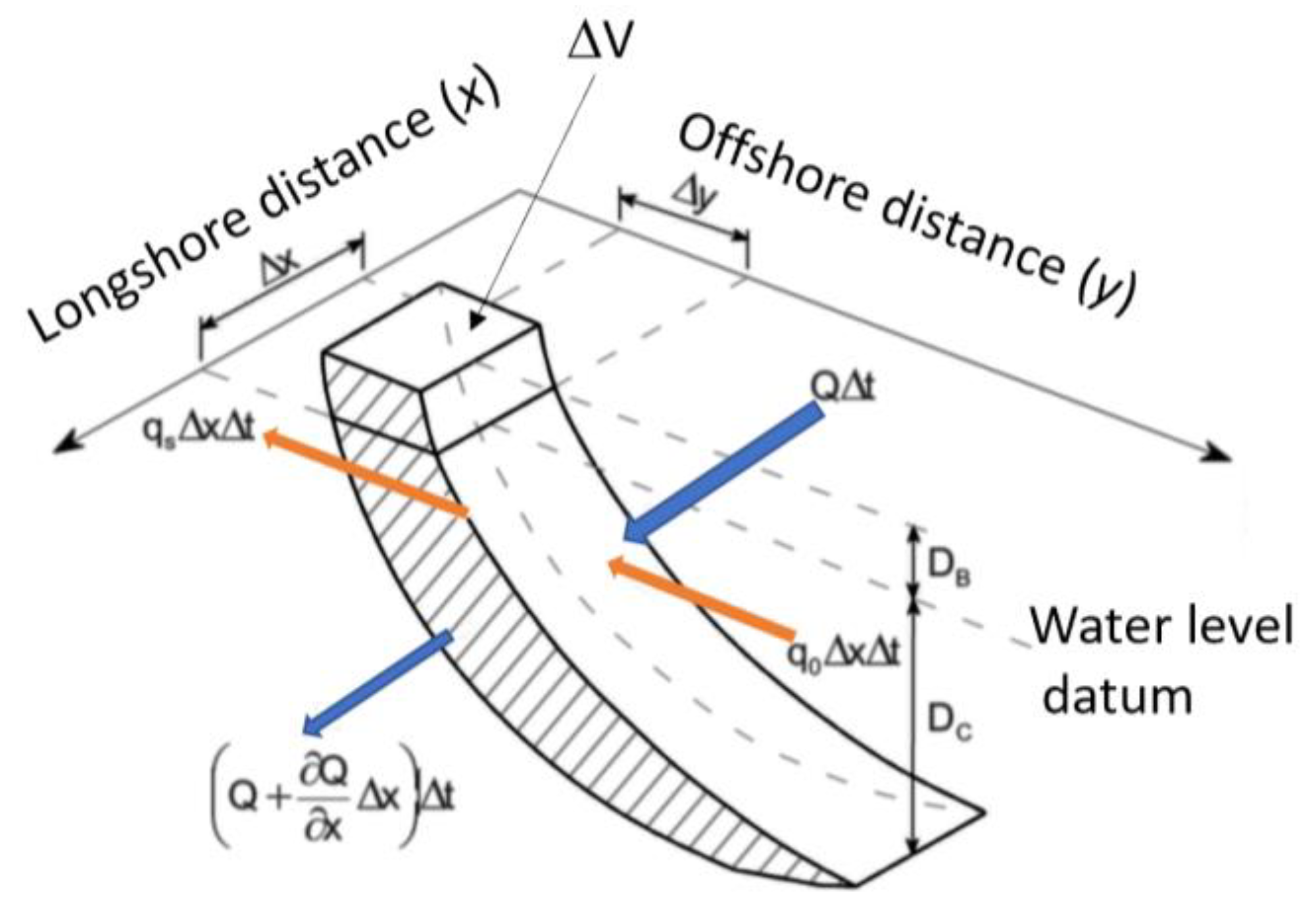
The explicit finite difference scheme solves the relationship between the longshore transport rate and shoreline accretion/erosion, which is caused by spatial and temporal variations in longshore transport. This relationship is formulated by the sediment continuity equation in a control volume, ΔV (Figure 12):

$$\frac{\mathsf{\Delta }V}{\mathsf{\Delta }t}(1-n)\left(D_b+D_c\right)+\frac{∆Q_{LT}}{∆x}=0$$

(8)

where $D_b$ is the berm height, $D_c$ is the closure depth, and $t$ is the time.

2.2.2. GSb Model Calibration

The $K_{GSb}$ coefficient depends on the longshore gradient in breaking wave height. In the present study, we adopted the $K_{GSb}$ coefficient obtained by [17], which was derived using high-quality shoreline data acquired from the Differential Global Positioning System (DGPS) for the Milford case study, covering a shorter alongshore stretch of 280 m (i.e., a more limited domain). Calibration was performed by comparing the observed and calculated shoreline evolution using $K_{GSb}$ values of 0.005, 0.01, 0.05, 0.1, and 0.2. The best agreement was obtained with a value of $K_{GSb}$ = 0.1, which resulted in the lowest root-mean-square error (RMSE) of 4.6. In the present case, which involves a beach with a single groin on a smooth and uniform bathymetry, the longshore gradient in breaking wave height is moderate. Consequently, the model outcomes are relatively sensitive to the value of $K_{GSb}$. Indeed, the differences among all the estimated RMSE values were less than 0.2.

2.2.3. GSb Model Setup

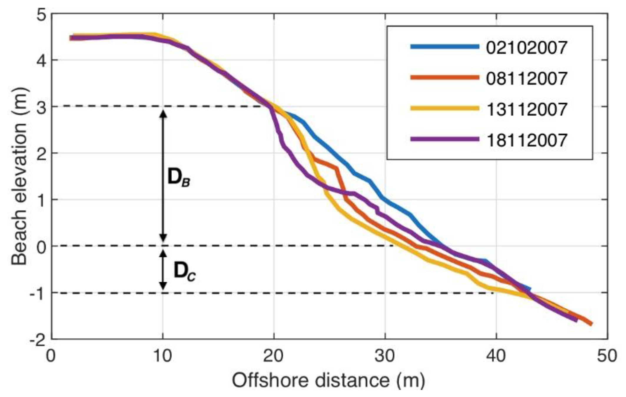
The first selected ARGUS shoreline available after the groin deployment (5 October 2007) was assumed as the initial shoreline. The values of closure depth and berm height, D_c and D_b, respectively, were selected equal to 1 m and 3 m, respectively, based on an accurate evaluation of the cross-shore beach profile evolution over time (Figure 13) [18]. The nominal diameter of the sediment equal to D_n50 = 11.19 mm was assumed. The computational domain was assumed to be 740 m long with a grid size of DX = 5 m and NX = 148. The groin was positioned at the $x$ coordinate = 250 m. The time step for the simulation was set to 0.05 h (180 s), and the total duration of simulation was 39 days. Following [44], fixed boundary conditions were used since they are far away from the groin (i.e., the length of the entire calculation domain is on the order of two or three groin length). It assures that the boundary conditions are unaffected by changes that take place in the vicinity of the groin.

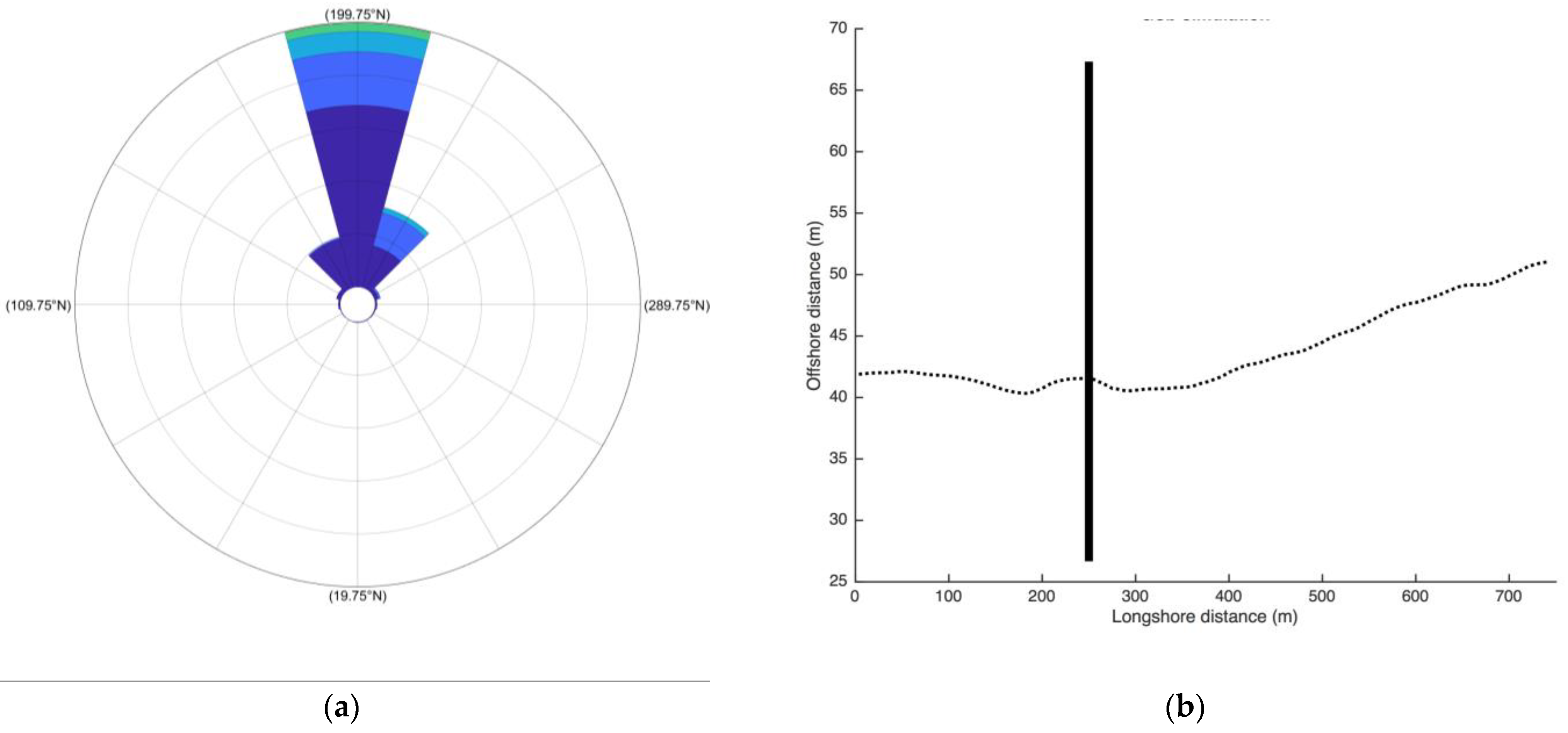
The initial shoreline and wave directions (AWAC and SWAN) were rotated by 199.75 degrees counterclockwise from the northing/easting grid, as shown in Figure 14, in order to adapt the input data with the numerical model convention, which requires the shoreline to be oriented towards the sea.

3. Numerical Results

Numerical simulations to investigate the morphodynamics response of a temporary groin deployed in the study area were performed. The predictive performance of the GSb model was evaluated by comparing the numerical results with the observed ARGUS shorelines in a 740 m long domain. To simulate the shoreline evolution, both nearshore observed AWAC data and numerical data propagated from offshore to nearshore using the SWAN numerical model were adopted as wave input for the GSb model.

3.1. ARGUS Shorelines and Nearshore Wave Data (AWAC)

GSb simulations were performed using the input mentioned in Section 2.2.3 and the nearshore AWAC wave data.

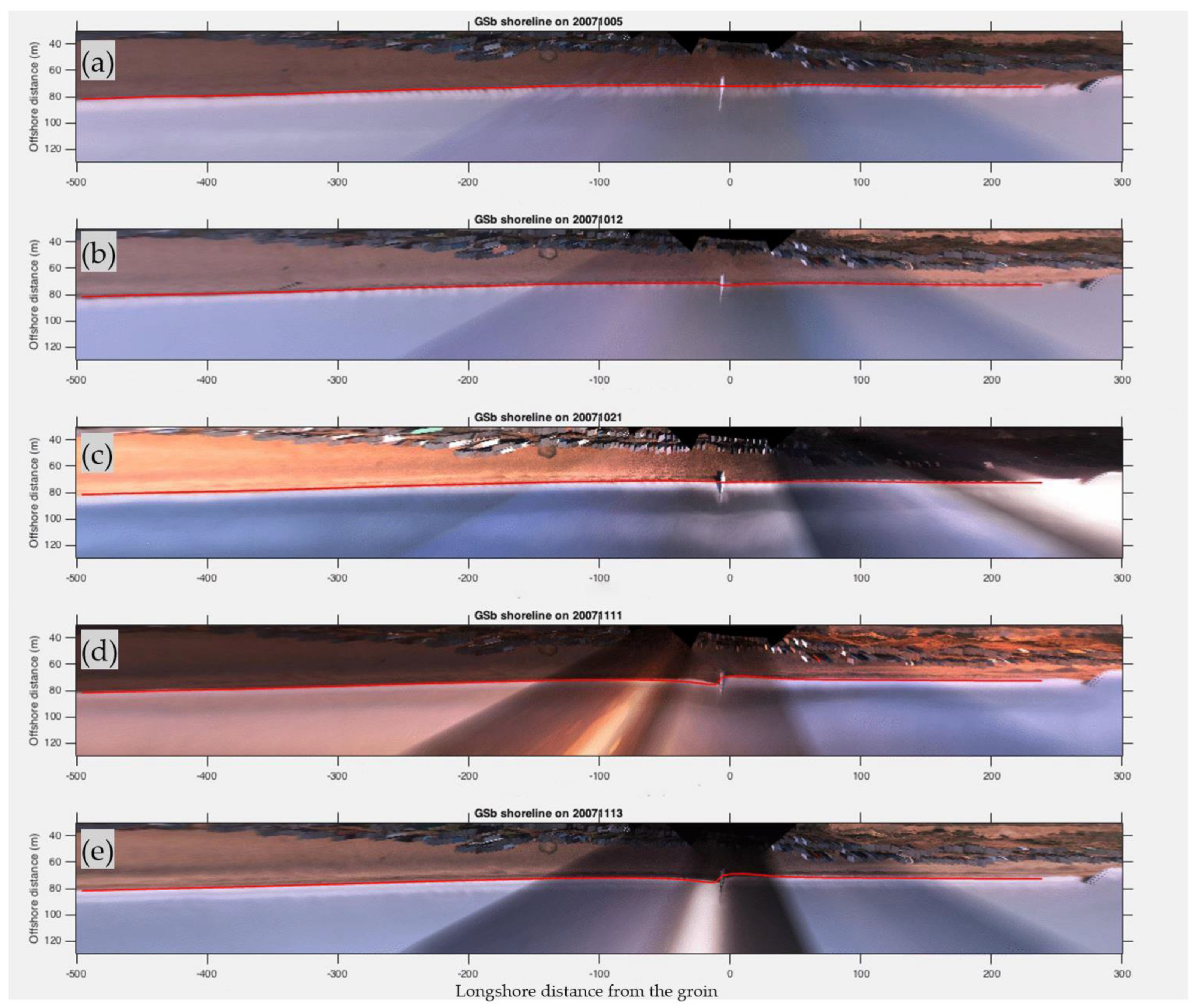
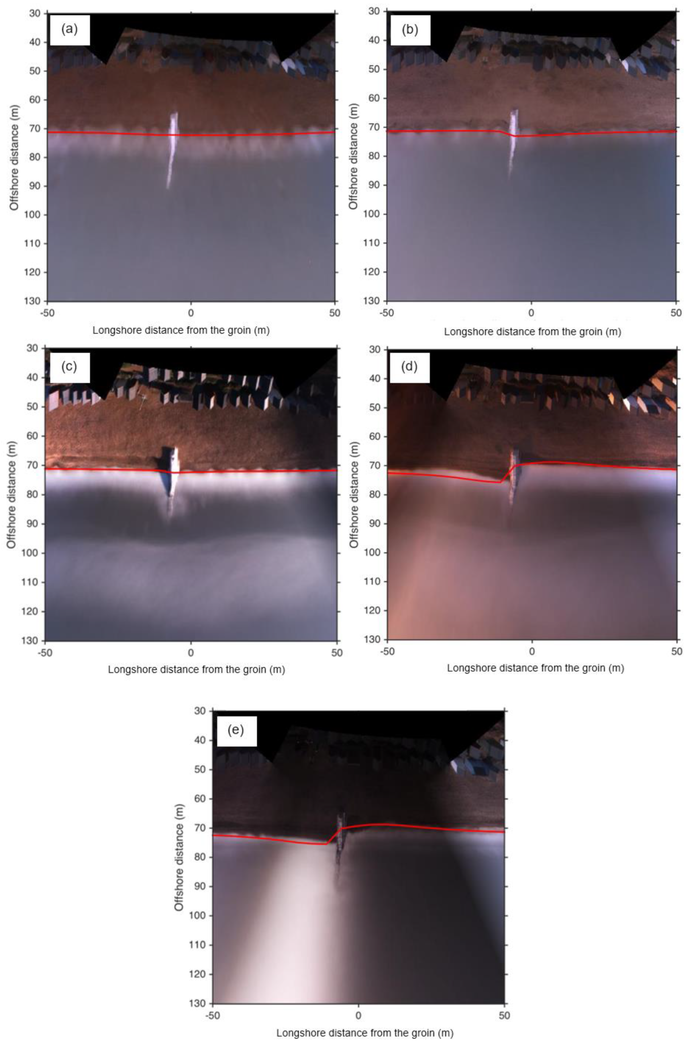
Figure 15a–e show the initial shoreline ((a) 5 October 2007) and the calculated shoreline compared with the ARGUS images on (b) 13 October 2007, (c) 21 October 2007, (d) 11 November 2007, and (e) 13 November 2007. Additionally, a more detailed view of the numerical results, on the same dates, in the vicinity of the groin is presented in Figure 16a–e.

The comparison of the calculated shorelines and the ARGUS images confirms the ability of the GSb model to predict the shoreline evolution in the presence of a groin under the influence of waves observed by the AWAC. In particular, the model accurately predicts the shoreline evolution at intermediate times in which shoreline advance occurs on the east side of the groin in the days until 12 October (Figure 15b and Figure 16b). Subsequently, the shoreline evolution trend is reversed, and a significant shoreline advance is observed on the west side of the groin from 11 November until the end of the simulation (Figure 15d,e and Figure 16d,e). These findings highlight the capacity of the GSb model to predict the day-to-day effects of wave attack on shoreline dynamics. According to the current literature, there are no other one-line numerical models capable of predicting the day-to-day shoreline evolution.

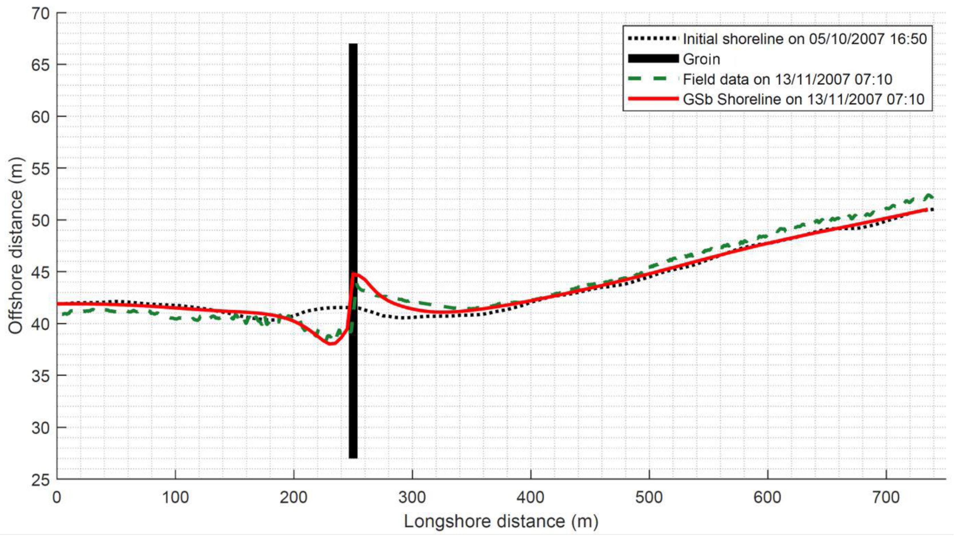
Figure 17 shows a comparison between the GSb shoreline (red line) and the observed ARGUS shoreline (green dotted line) at the end of numerical simulation (13 November 2007), 39 days after the groin deployment.

The result demonstrates the capability of the GSb model to predict the accretion/erosion that occurred up-drift/down-drift of the groin using the nearshore AWAC wave data. However, the calculated accretion on the up-drift side of the groin is slightly overestimated.

3.2. ARGUS Shorelines and Nearshore Propagated SWAN Wave Data

GSb simulations were performed using the input mentioned in Section 2.2.3 and the nearshore wave characteristics obtained from the SWAN model (as described in Section 2.1.6).

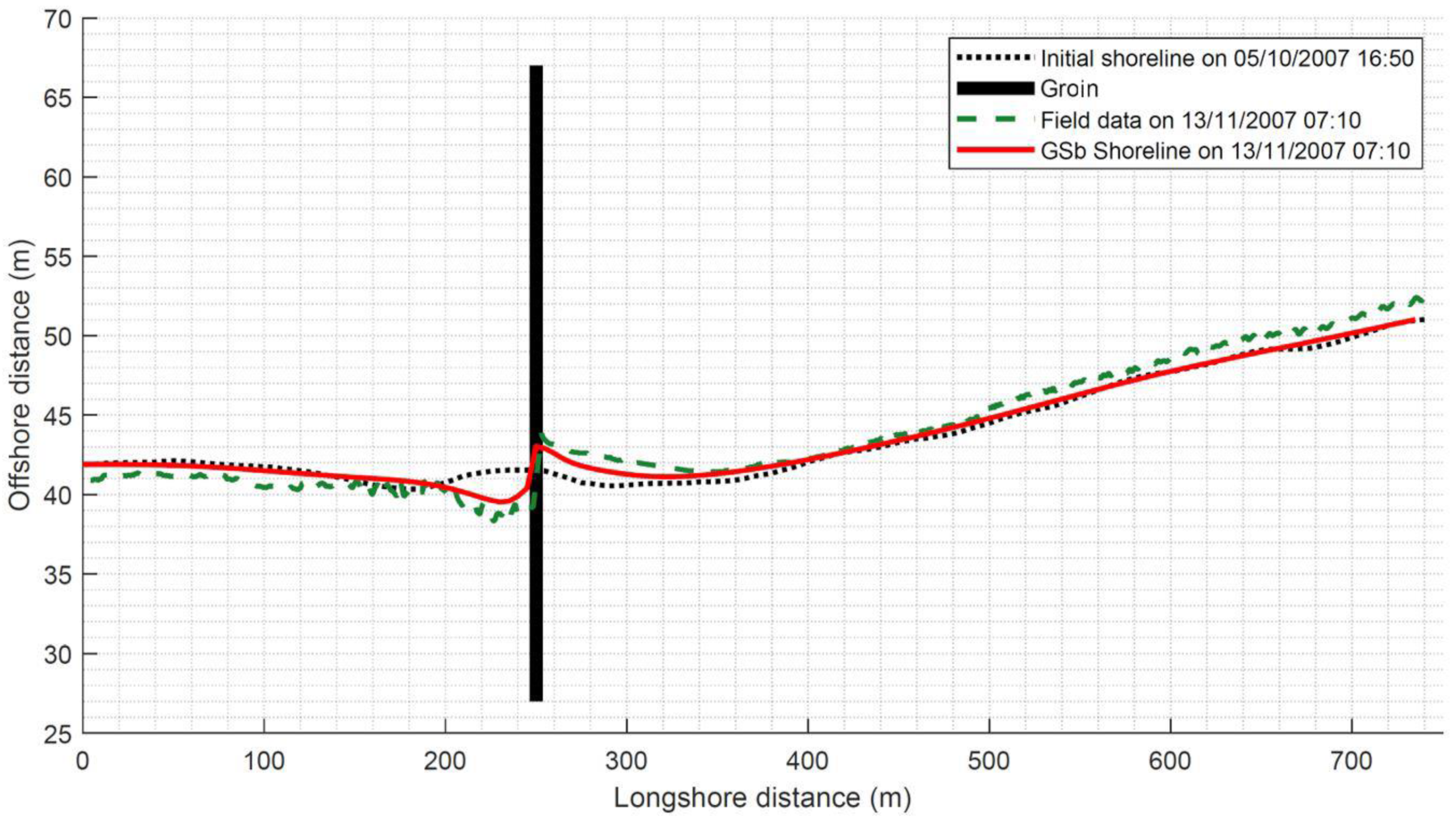
Figure 18 shows a comparison between the GSb shoreline (red line) and the observed ARGUS shoreline (green dotted line) at the end of numerical simulation (13 November 2007), 39 days after the groin deployment.

Result demonstrates the capability of the model to predict the accretion/erosion that occurred up-drift/down-drift of the groin using the nearshore wave characteristics obtained from the SWAN model. However, the calculated accretion/erosion on the up-drift/down-drift sides of the groin is slightly underestimated.

4. Discussion and Conclusions

In the present paper, the reliability of a recent one-line model called the General Shoreline beach (GSb) model has been verified using field data. The GSb model, unlike the other one-line models that require two calibration coefficients ($K_1$ and $K_2$), requires only one calibration coefficient, $K_{GSb}$, which simplifies its use significantly. In particular, for a model with two calibration coefficients, initial values are chosen and simulations are run to match observed data through iterative parameter adjustments. The process is simpler for a model with only one calibration coefficient where an initial value is chosen and the coefficient is iteratively adjusted to match observed data through simulations. Moreover, $K_{GSb}$ does not depend on sediment grain size but only on the longshore gradient in breaking wave height. This property makes the calibration process of the GSb model more efficient, allowing for more precise simulations of coastal morphodynamics.

The numerical simulations were performed using high-resolution shoreline data observed from an ARGUS monitoring station during a field experiment conducted in Milford-on-Sea, UK. A temporary groin was deployed to evaluate the shoreline evolution on a mixed beach. Both nearshore waves observed by the AWAC profiler and propagated waves from offshore (CCO buoy location) to nearshore using the SWAN numerical model have been adopted as GSb wave input data.

The results demonstrate the effectiveness of the GSb online numerical model in accurately predicting day-to-day changes in shoreline dynamics resulting from wave attack. The model has been capable of predicting patterns of accretion/erosion that occurred up-drift and down-drift of the groin, using both observed nearshore wave characteristics collected from AWAC and those obtained from the SWAN model. In the case of AWAC data, the model slightly overestimated the calculated accretion on the up-drift side of the groin. When using nearshore SWAN model data, the GSb model accurately predicted the shoreline advance/retreat.

Appendix B and C present the full high-resolution dataset of ARGUS images and wave data used in the present study, which represent a valuable resource for coastal researchers to further evaluate and improve numerical models of coastal morphodynamics.

One possible direction for future research could be to further refine the GSb model by incorporating additional factors that can influence shoreline dynamics, such as storm surges and sea level rise. Another potential avenue for future research is to investigate the effectiveness of different types of coastal protection measures in different environmental conditions, using the GSb model to simulate the effects of various design parameters on shoreline evolution. Overall, the findings of the present study have important implications for coastal management and highlight the need for continued research into the complex processes that govern shoreline evolution.

References

1. Pörtner, H.-O.; Roberts, D.C.; Masson-Delmotte, V.; Zhai, P.; Tignor, M.; Poloczanska, E.; Mintenbeck, K.; Nicolai, M.; Okem, A.; Petzold, J. IPCC special report on the ocean and cryosphere in a changing climate. IPCC Intergov. Panel Clim. Chang. Geneva Switz. 2019, 1. [Google Scholar] [CrossRef]
2. D’Alpaos, A.; Lanzoni, S.; Marani, M.; Rinaldo, A. Landscape evolution in tidal embayments: Modeling the interplay of erosion, sedimentation, and vegetation dynamics. J. Geophys. Res. Earth Surf. 2007, 112. [Google Scholar] [CrossRef]
3. Ashton, A.D.; Murray, A.B. High-angle wave instability and emergent shoreline shapes: 1. Modeling of sand waves, flying spits, and capes. J. Geophys. Res. Earth Surf. 2006, 111. [Google Scholar] [CrossRef]
4. Shi, H.; Yu, X. An effective Euler-Lagrange model for suspended sediment transport by open channel flows. Int. J. Sediment Res. 2015, 30, 361–370. [Google Scholar] [CrossRef]
5. Guan, X.; Shi, H. Translational momentum of deformable submarine landslides off a slope. J. Fluid Mech. 2023, 960, A23. [Google Scholar] [CrossRef]
6. Hanson, H.; Kraus, N.C. GENESIS: Generalized Model for Simulating Shoreline Change. Report 1. Technical Reference; Coastal Engineering Research Center: Vicksburg, MS, USA, 1989. [Google Scholar]
7. Blanco, B. Beachplan (Version 04.01) Model Description; HR Wallingford Report: Wallingford, UK, 2003. [Google Scholar]
8. González, M.; Medina, R.; González-Ondina, J.; Osorio, A.; Méndez, F.; García, E. An integrated coastal modeling system for analyzing beach processes and beach restoration projects, SMC. Comput. Geosci. 2007, 33, 916–931. [Google Scholar] [CrossRef]
9. Frey, A.E.; Connell, K.J.; Hanson, H.; Larson, M.; Thomas, R.C.; Munger, S.; Zundel, A. GenCade Version 1 Model Theory and User’s Guide; Engineer Research and Development Center Vicksburg Ms Coastal Inlets: Vicksburg, MS, USA, 2012. [Google Scholar]
10. D’Alessandro, F.; Tomasicchio, G.R.; Musci, F.; Ricca, A. Dune erosion physical, analytical and numerical modelling. In Proceedings of the 33rd Conference on Coastal Engineering, Santander, Spain, 1–6 July 2012. 12/14, p. sediment.32. [Google Scholar]
11. Sutherland, J.; Walstra, D.J.R.; Chesher, T.J.; van Rijn, L.C.; Southgate, H.N. Evaluation of coastal area modelling systems at an estuary mouth. Coast. Eng. 2004, 51, 119–142. [Google Scholar] [CrossRef]
12. Elias, E.P.L.; Walstra, D.J.R.; Roelvink, J.A.; Stive, M.J.F.; Klein, M.D. Hydrodynamic Validation of Delft3D with Field Measurements at Egmond. In Proceedings of the Conference Information 27th International Conference on Coastal Engineering (ICCE), Sydney, Australia, 16–21 July 2000; pp. 2714–2727. [Google Scholar]
13. Kamphuis, J. Marketing uncertainty. In Proceedings of the International Conference on Coastal and Port Engineering in Developing Countries (COPEDEC), Cape Town, South Africa, 19–23 April 1999; pp. 2088–2099. [Google Scholar]
14. Dabees, M.; Kamphuis, J.W. ONELINE, a numerical model for shoreline change. In Proceedings of the Conference Information 26th International Conference on Coastal Engineering, Copenhagen, Denmark, 22–26 June 1998; pp. 2668–2681. [Google Scholar]
15. Güner, H.A.A.; Yüksel, Y.; Çevik, E.Ö. Determination of longshore sediment transport and modelling of shoreline change. In Sediment Transport; In tech open: London, UK, 2011. [Google Scholar] [CrossRef]
16. Francone, A. New One-Line Model for Shoreline Evolution at Beaches Composed of not Cohesive Grains of Any Size. Ph.D. Thesis, University of Calabria, Arcavacata di Rende, Italy, 2020. [Google Scholar] [CrossRef]
17. Tomasicchio, G.R.; Francone, A.; Simmonds, D.J.; D’Alessandro, F.; Frega, F. Prediction of shoreline evolution. Reliability of a general model for the mixed beach case. J. Mar. Sci. Eng. 2020, 8, 361. [Google Scholar] [CrossRef]
18. Martín-Grandes, I.; Hughes, J.; Simmonds, D.J.; Chadwick, A.J.; Reeve, D.E. Novel methodology for one line model calibration using impoundment on mixed beach. In Proceedings of Coastal Dynamics 2009: Impacts of Human Activities on Dynamic Coastal Processes (With CD-ROM); World Scientific: Singapore, 2009; pp. 1–10. [Google Scholar]
19. Martín Grandes, I. Understanding Longshore Sediment Transport on a Mixed Beach. Ph.D. Thesis, Plymouth University, Plymouth, UK, 2015. [Google Scholar]
20. Martin-Grandes, I.; Simmonds, D.J.; Karunarathna, H.; Horrillo-Caraballo, J.M.; Reeve, D.E. Assessing the Variability of Longshore Transport Rate Coefficient on a Mixed Beach. In Proceedings of the Coastal Dynamics, Helsingør, Denmark, 12–16 June 2017; pp. 12–16. [Google Scholar]
21. Carter, D.; Bray, M.; Hooke, J. SCOPAC Sediment Transport Study; Environment Agency: Bristol, UK, 2012. [Google Scholar]
22. Seymour, R.J. Cross-Shore Sediment Transport. In Encyclopedia of Coastal Science; Schwartz, M.L., Ed.; Springer: Dordrecht, The Netherlands, 2005; pp. 352–353. [Google Scholar]
23. Bodge, K.R. Short Term Impoundment of Longshore Sediment Transport (Coastal Engineering); University of Florida: Gainesville, FL, USA, 1986. [Google Scholar]
24. Wang, P.; Kraus, N.C. Longshore sediment transport rate measured by short-term impoundment. J. Waterw. Port Coast. Ocean Eng. 1999, 125, 118–126. [Google Scholar] [CrossRef]
25. Van Wellen, E.; Chadwick, A.; Mason, T. A review and assessment of longshore sediment transport equations for coarse-grained beaches. Coast. Eng. 2000, 40, 243–275. [Google Scholar] [CrossRef]
26. Bodge, K.R.; Dean, R.G. Short-term impoundment of longshore transport. In Proceedings of the Coastal Sediments, New Orleans, LA, USA, 12–14 May 1987; pp. 468–483. [Google Scholar]
27. Plant, N.G.; Holman, R.A. Intertidal beach profile estimation using video images. Mar. Geol. 1997, 140, 1–24. [Google Scholar] [CrossRef]
28. Aarninkhof, S.G.J. Nearshore Bathymetry Derived from Video Imagery. Ph.D. Thesis, Delft University, Delft, The Netherlands, 2003. [Google Scholar]
29. Dalyander, P.; Holman, R. Quantification of nearshore morphology based on video imaging. Mar. Geol. 2004, 208, 101–111. [Google Scholar]
30. Holman, R.A.; Stanley, J. The history and technical capabilities of Argus. Coast. Eng. 2007, 54, 477–491. [Google Scholar] [CrossRef]
31. Booij, N.; Holthuijsen, L.; Ris, R. The "SWAN" wave model for shallow water. In Coastal Engineering 1996; American Society of Civil Engineers: Orlando, FL, USA, 1996; pp. 668–676. [Google Scholar]
32. Pelnard-Considère, R. Essai de théorie de l’évolution des formes de rivage en plages de sable et de galets. J. L’hydraul. 1957, 4, 289–298. [Google Scholar]
33. Bruun, P. Coast Erosion and the Development of Beach Profiles; US Beach Erosion Board. Technical memorandum (United States. Beach Erosion Board): Washington, DC, USA, 1954; Volume 44. [Google Scholar]
34. Dean, R.G. Equilibrium Beach Profiles: US Atlantic and Gulf Coasts; Department of Civil Engineering, University of Delaware: Newark, Delaware, 1977. [Google Scholar]
35. Ozasa, H.; Brampton, A. Mathematical modelling of beaches backed by seawalls. Coast. Eng. 1980, 4, 47–63. [Google Scholar] [CrossRef]
36. Medellín, G.; Torres-Freyermuth, A.; Tomasicchio, G.R.; Francone, A.; Tereszkiewicz, P.A.; Lusito, L.; Palemón-Arcos, L.; López, J. Field and numerical study of resistance and resilience on a sea breeze dominated beach in Yucatan (Mexico). Water 2018, 10, 1806. [Google Scholar] [CrossRef]
37. Hamza, W.; Tomasicchio, G.R.; Ligorio, F.; Lusito, L.; Francone, A. A Nourishment Performance Index for Beach Erosion/Accretion at Saadiyat Island in Abu Dhabi. J. Mar. Sci. Eng. 2019, 7, 173. [Google Scholar] [CrossRef]
38. Goda, Y.; Takayama, T.; Suzuki, Y. Diffraction diagrams for directional random waves. In Proceedings of the Conference Information 16th International Conference on Coastal Engineering, Hamburg, Germany, 27 August–3 September 1978; pp. 628–650. [Google Scholar]
39. Tomasicchio, G.R.; Francone, A.; Salvadori, G. On the General Longshore Transport model for resilient beaches. Coast. Eng. 2023, 180, 104257. [Google Scholar] [CrossRef]
40. Lamberti, A.; Tomasicchio, G.R. Stone mobility and longshore transport at reshaping breakwaters. Coast. Eng. 1997, 29, 263–289. [Google Scholar] [CrossRef]
41. Tomasicchio, G.R.; D’Alessandro, F.; Barbaro, G.; Musci, E.; De Giosa, T.M. Longshore transport at shingle beaches: An independent verification of the general model. Coast. Eng. 2015, 104, 69–75. [Google Scholar] [CrossRef]
42. Tomasicchio, G.R.; D’Alessandro, F.; Frega, F.; Francone, A.; Ligorio, F. Recent improvements for estimation of longshore transport. Ital. J. Eng. Geol. Environ. 2018, 2018, 179–187. [Google Scholar] [CrossRef]
43. Tomasicchio, G.; Lamberti, A.; Guiducci, F. Stone movement on a reshaped profile. In Proceedings of the Conference Information 24th International Conference on Coastal Engineering, Kobe, Japan, 23–28 October 1994; pp. 1625–1640. [Google Scholar]
44. USACE. Shore Protection Manual; Dept. of the Army, Waterways Experiment Station, Corps of Engineers, Coastal Engineering Research Center: Vicksburg, MS, USA; Washington, DC, USA, 1984. [Google Scholar]
Figure 1. Study area location (from Earthstar Geographics maps).
Jmse 11 01037 g001
Figure 2. Percentage of material passing through the sieve for three different samples: fine, coarse, and the total sample.
Jmse 11 01037 g002
Figure 3. Pictures from the top of Hordle Cliff of (a) groin construction, filling the geobags during low tide on 27 September 2007; (b) view of the temporary structure deployed at Milford-On-Sea.
Jmse 11 01037 g003
Figure 4. ARGUS images: (a) 1 October 2007 16:50; (b) 2 October 2007 09:30; (c) 3 October 2007 06:30; (d) 4 October 2007 13:50; and (e) 5 October 2007 15:50.
Jmse 11 01037 g004
Figure 5. AWAC wave data from 1 October 2007 to 25 November 2007: (a) time series of significant height, wave angle, and peak period; (b) wave rose and mean shoreline orientation.
Jmse 11 01037 g005
Figure 6. CCO wave data from 1 October 2007 to 25 November 2007: (a) time series of significant height, wave angle, and peak period; (b) wave rose and mean shoreline orientation.
Jmse 11 01037 g006
Figure 7. Groin, AWAC, and Waverider Buoy (CCO) locations.
Jmse 11 01037 g007
Figure 8. (a) Area of interest and corner grid point EMODNET bathymetry portal; (b) contour plot of EMODNET bathymetry (units in meters).
Jmse 11 01037 g008
Figure 9. The 3D mesh plot. Red circle reperesent Buoy location and red asterisk represent AWAC location.
Jmse 11 01037 g009
Figure 10. Wave rose of (a) AWAC data and (b) SWAN data obtained after wave propagation from the buoy location (1500 m offshore, 10 m water depth) to the AWAC location (600 m offshore, 7 m water depth).
Jmse 11 01037 g010
Figure 11. Observed (red line) and computed (blue line) significant wave height.
Jmse 11 01037 g011
Figure 12. Sketch for shoreline change calculation in the one-line model (adapted from [6]).
Jmse 11 01037 g012
Figure 13. Surveyed cross-shore beach profile at Milford-on-Sea.
Jmse 11 01037 g013
Figure 14. GSb model setup: (a) wave data and (b) initial shoreline (5 October 2007).
Jmse 11 01037 g014
Figure 15. Comparison between calculated shoreline and ARGUS images: (a) 5 October 2007, (b) 13 October 2007, (c) 21 October 2007, (d) 11 November 2007, and (e) 13 November 2007.
Jmse 11 01037 g015
Figure 16. Comparison between calculated shoreline and ARGUS images in the groin area for (a) 5 October 2007, (b) 13 October 2007, (c) 21 October 2007, (d) 11 November 2007, and (e) 13 November 2007.
Jmse 11 01037 g016
Figure 17. Comparison between the GSb shoreline (red line) and the observed ARGUS shoreline (green dotted line) at the end of numerical simulation (13 November 2007), 39 days after the groin deployment, in the case of nearshore AWAC wave input.
Jmse 11 01037 g017
Figure 18. Comparison between the GSb shoreline (red line) and the observed ARGUS shoreline (green dotted line) at the end of numerical simulation (13 November 2007), 39 days after the groin deployment, in the case of nearshore SWAN wave input.
Jmse 11 01037 g018