Abstract
A regional wave forecasting system in East Asia, including the Korean Peninsula, was built based on WAVEWATCH III using offshore wind forecast data from the Global Data Assimilation Prediction System. The numerical simulations were performed on the sensitivity of the interaction between input wind and wave development. The forecasts for each condition were compared and verified with the observational data of marine meteorological buoys from 1 August to 30 September 2020. The sensitivity conditions were configured to have a specific range of variables related to the directional distribution of input winds (SINA0) and variables indicating the development of input wind–wave (CDFAC) in the ST6. The results were presented by calculating the mean error and root mean square error for all observation points. Overall, as the CDFAC increased, the mean error tended to decrease according to the forecast time and the root mean square error increased. Although the effect of SINA0 at the same CDFAC was insignificant, when SINA0 increased in sections where the significant wave height decreased rapidly, the significant wave height tended to decrease. In addition, the main variables that affect the physical process of wind–wave interaction should be considered to improve wave model forecasting performance and accuracy.
1. Introduction
Wave models were developed to numerically simulate the growth, propagation, and decay of ocean waves using offshore input data of atmospheric models. In recent years, third-generation wave models based on wave spectrum analysis have been developed and, over the generations, their forecasting performance and accuracy have been significantly improved through advancements in computing algorithms [1,2,3,4,5,6,7,8,9]. In addition, high-performance computing based on large-scale computational resources allowed us to process computing tasks more quickly, and economic and precise numerical simulations of complex natural phenomena have become possible through coupling between sophisticated numerical models [10,11,12]. Therefore, many institutions and research groups use wave models to produce forecast information, use them for forecasting work, and apply them in research and engineering related to wave behavior characteristics [13,14,15,16,17].
Observation technologies are rapidly developing along with the improvement of numerical modeling techniques, and high-quality observation data are being produced using various types of equipment. Observation data are used as verification data to improve the performance of numerical models and evaluate their accuracy in wave forecast modeling. In general, observations allow us to identify wave specifications, such as significant wave height, wave direction, and wave period, as well as offshore wind specifications, such as wind speed and direction, which are evaluation factors essential for validating wave models [18,19]. In recent years, more and more data observed by satellites and marine meteorological buoys are being used. Many academic studies have used wave specifications observed by satellites to perform numerical modeling and verify the forecasting performance of wave models [20,21,22]. The scatterometer data were used to provide the wind forcing at the center of cyclones in the South Atlantic for improving the WW3 performance [23]. The development of numerical modeling and observation techniques has enabled us to explain the overall physical mechanism of waves, from growth, propagation, and dissipation. In addition, wave models have been refined with improvements in nonlinear wave interactions, making them applicable in various academic fields, including wave forecasting [24,25].
WAVEWATCH III (WW3), a representative third-generation wave model in wave forecasting, calculates the spectral energy balance equation below (Equation (2)) [26].
where the wave action density spectrum in Equation (1) is derived from the wavenumber–direction spectrum function expressed in terms of the wavenumber , the direction , the radian frequency , and denotes the pure source function for spectrum . In general, the entire pure source function is divided into , , and in deep waters, where denotes energy input by wind, represents nonlinear energy transfer by wave–wave interaction, indicates energy dissipation, and is user define function, respectively (Equation (3)). As such, wave models include various physical processes considering nonlinear wave interactions, bottom and surface friction effects, and input wind fields. These combinations allow us to more closely understand the entire physical process of wave development and dissipation. Recently, a wave analysis physics package based on observations was developed [6,8], and the accuracy and wave forecast performance of numerical simulations have improved as the physical mechanism for nonlinear wave interactions has improved by comparison study between physical packages in WW3 [27,28]. The resolution of computational domains increased with the improvement of wave models, and the development of data assimilation and numerical simulation techniques contributed to gradually improving the forecasting performance [29,30,31,32,33]. More complex wave behavior characteristics can be analyzed by applying coupling techniques between models.
However, unlike weather models, wave models are highly dependent on the forecasting accuracy of input data in model performance. In addition, numerical simulations on sensitivity are needed because their forecasting performance and accuracy are affected by the spatial and temporal resolution of the model and the wind–wave physics mechanism. In particular, sensitivity numerical simulations for the parameters included in the physics package are performed to optimize the wave model by considering the state of offshore wind input data, topographical characteristics, and grid structure [34,35,36,37]. A wave model’s physics package consists of many physical parameters related to wave development parameters, propagation and dissipation, and nonlinear effects by offshore wind. The combination of these parameters determines the forecasting performance of the model. However, performing numerical tests on the sensitivity of all parameters related to forecasting performance is inefficient. Therefore, sensitivity analysis should be preceded for physical parameters closely related to offshore wind–wave development and nonlinear wave interactions, which are known to have the most significant impact on forecasting performance, and then gradually examine the interaction between parameters [38,39,40,41].
This study used the offshore wind forecast data of a high-resolution Korean global atmospheric model to forecast waves in East Asia, including the Korean Peninsula, and evaluated the model’s forecasting performance from 1 August 2020, 00 UTC to 30 September 2020, 12 UTC. This period included rapid atmospheric changes as “Maysak” and “Haishen” typhoons landed on the Korean Peninsula in succession and caused great damage. A wave model was developed based on the ST6 physics package. Sensitivity numerical simulations were run to determine the offshore wind input data and physical parameters suitable for the model environment. Based on the sensitivity numerical simulation results, the wave model’s forecasting performance according to the quality and forecast time of the input offshore wind was verified by comparing it with the data observed by ocean data buoys of the Korea Meteorological Administration (KMA). In addition, the wave model was optimized by investigating how changing the physical parameters affects the forecasting performance.
2. Methodology
2.1. ST6 Source Term
The WW3 wave model includes a physics package that combines parameterizations of physical processes and various source terms to explain complex wave phenomena, such as wind–wave interaction, nonlinear wave–wave interaction, white-capping, surf-breaking, bottom friction, and swell. As these physical variables influence each other, it is necessary to optimize the wave model by applying an appropriate physics package to suit various numerical modeling environments. These include the quality of the input wind field and the type of coupled model to minimize forecast errors and quickly calculate a higher-resolution model. Therefore, in this study, a wave forecasting system was constructed by applying the ST6 physics package [6,8], and numerical simulations of physical variable sensitivity were conducted through actual forecasting cases [42,43].
The ST6 physics has physical characteristics for wind–wave exchange, including complete air-flow separation leading to a relative decrease in input wind under strong wind and steep wave conditions and the wave growth dependence of wave steepness by nonlinear behavior. In particular, in the formula of the input source term (), the directional distribution of the input wind field that directly affects the wind–wave growth term is shown in Equation (4). The directional distribution for the input wind field is defined as the sum of Equations (5) and (6), and each is divided into favorable winds and adverse winds, respectively [26].
where is the directional distribution, is the favorable winds, is the adverse winds, is the tuning parameter, is the scaling wind speed ( where is the wind speed at a 10 m height and is the friction velocity), is the wind-wave angle difference, and is the phase velocity.
The normal stress acting on the water surface for the interaction between the atmospheric boundary layer and the ocean surface, which is significant in calculating the moment flex, was expressed as the sum of viscous and wave-supported stress. The total stress on the boundary layer is calculated by a combination of wind speed , density , and drag coefficient and is parameterized by Equations (7) and (8) [44].
In Equation (4), (SINA0) adjusts the sum of favorable winds and adverse wind components that determine the directional distribution (), and (CDFAC) is the drag coefficient that reduces the bias of the input wind and is an important parameter that determines a wave model’s forecasting performance.
A wave model’s forecasting performance varies depending on the forecasting accuracy of offshore wind. However, we can improve the performance and optimize the model for the input offshore wind by correcting these physical variables. As each physical variable organically affects and interacts with each other, these relationships need to be examined through numerical simulations on the sensitivity of model variables.
This study configured numerical simulations on the sensitivity of main variables as follows and compared and analyzed the forecasting performance results. Experimental cases were developed by limiting the wave growth coefficient and dissipation coefficient, which are the physical variables expected to respond most sensitively to the offshore input data to a specific range. CDFAC was changed from 0.8 to 1.2 in increments of 0.1. When CDFAC was 1.0, SINA0 was changed to 0.05, 0.10, and 0.15 and the wave model was performed using the same input wind. Although many physical variables make up a wave model, this study focused on comparing the physical variables related to wave growth, which are known to have the most significant impact on forecasting wave height. Follow-up studies will analyze the effect of changes in various physical variables on the forecasting results of wave models.
2.2. Numerical Model Set-Up
The calculation domain of the wave model built based on WW3 was from 20° to 50° in latitude and from 115° to 150° in longitude (Figure 1). The ETOPO1 of the National Geophysical Data Center (NGDC) was used as the ocean depth grid and coastline data from the Global Self-consistent Hierarchical High-resolution Shoreline (GSHHS) were used.
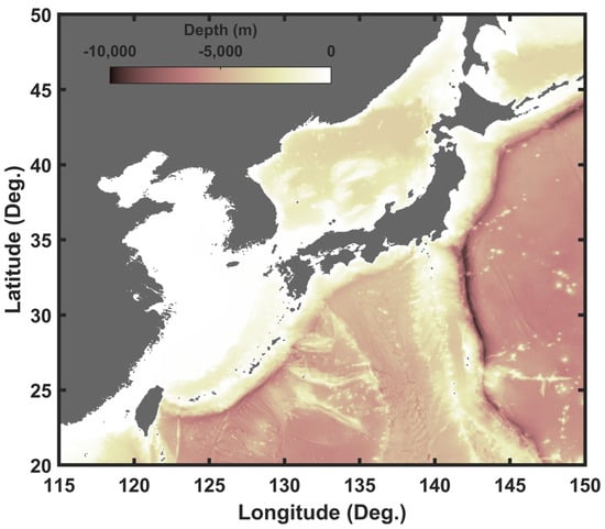
Figure 1.
Numerical model domain and bathymetry data.
Table 1 summarizes the wave model’s specifications. The wave model was run twice a day (00 UTC and 12 UTC) using the offshore wind forecasting results of the Korea Integrate Model and forecasted up to 120 h from its execution. The model’s initial conditions use the forecasting results by running the model 12 h in advance, and the boundary field used the forecasting results in the boundary region of this wave model by running a global wave model in advance. The global wave model for creating the boundary field was designed to assimilate data from five satellite observations and significant wave heights observed from marine meteorological buoys 24 h before running the model to reflect them in wave forecasts. The operating and calculation environment of the wave model for sensitivity numerical simulations was the same for all experimental conditions.

Table 1.
Numerical model description.
2.3. Observation Data
Figure 2 shows the installation locations and ID numbers of the meteorological buoys. The data observed by 18 marine meteorological buoys of KMA at 30 min intervals were used to verify the forecasting performance and sensitivity numerical simulations of the wave model in this study. The observation data to validate the wave model only comprised data that went through quality control rather than raw data. Missing data and abnormal observations were also excluded. The observation data after quality control were assumed to be true values for validating the wave model’s forecast results. Furthermore, since most of the buoy data are observed at a height of less than 5 m, it is considered that they include a prediction error according to the observation height when compared to the wind field of 10 m height used in the wave model.
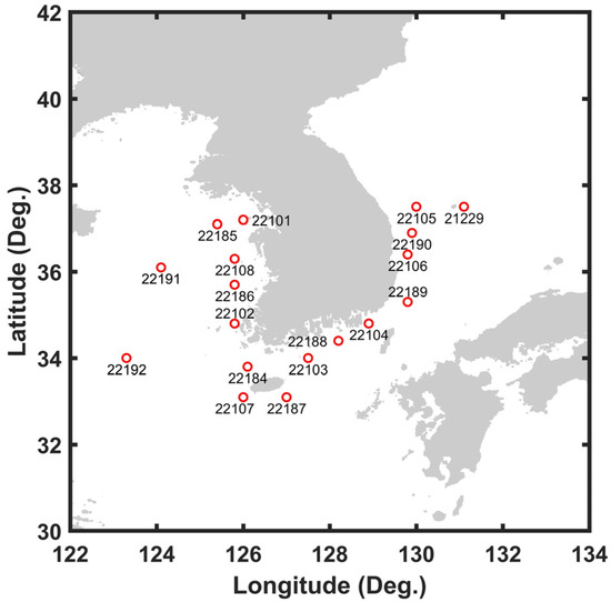
Figure 2.
ID number and locations (red circles) of marine meteorological buoys managed by KMA.
In addition to significant wave height, meteorological buoys provide real-time observation data, such as wind speed, wind direction, wave period, wave direction, and atmospheric pressure, which facilitate understanding of the rapidly changing marine weather conditions around the Korean Peninsula. Observation data that have undergone quality control are used to verify the forecasting performance and accuracy of numerical models and are useful in various research fields.
2.4. Validation Method
The validation period was from 1 August 2020, 00 UTC to 30 September 2020, 12 UTC. This period was particularly optimal for validating the wave model’s forecasting performance, as it included rapid atmospheric changes as two typhoons passed through the Korean Peninsula.
The significant wave height observed by marine meteorological buoys and the significant wave height predicted by the model were compared and analyzed to verify the wave model’s forecasting performance. Mean error and root mean square error were used as verification indicators, and significant wave heights were extracted and analyzed for each forecasting time for the locations of the marine meteorological buoys. The mean error is widely used in model validation because it can indicate whether the model tends to underestimate or overestimate by comparing it with observed values. The root mean square error is an indicator that can quantitatively identify the error between the observed and predicted value. The mean error and root mean square error are interpolated from the model grid point to the buoy observation position to calculate the verification index at the observation position. It is then compared with the observation results collected at all buoy positions for each forecasting time and calculated through Equations (9) and (10).
where is predicted value, is observed value, and is a number of samples [45]. The effect of changes in the ST6 physical variables on the forecasting performance was investigated by comparing the bias and RMSE for each forecasting time calculated according to the sensitivity test conditions.
3. Results
3.1. Analysis of the Relationship between Observed Offshore Wind and Significant Wave Height
The correlation between the observed offshore wind and wave height and its characteristics were analyzed before validating the wave model’s forecasting performance. As the development and propagation of waves are generally most affected by offshore winds, we first analyzed the observation data to understand the physical correlation between offshore winds and waves.
Figure 3 shows the offshore wind and significant wave height observed by marine meteorological buoys according to each mean period (+). In all four buoy points shown in the figure, high significant wave heights were observed when the wave period was relatively large and the observation frequency was high. Relatively high waves developed when the offshore wind speed increased. For waves with a wave period of 10 s or less, a significant wave height of 5 m or less was observed in sections with a wind speed of less than 15 m/s, and high significant wave heights were observed when the wave period was 10 s or more. Analyzing the observation data showed that the influence of offshore wind was dominant in wave development. Therefore, sufficient analysis of the dynamics between wave development and offshore wind should be preceded in wave model forecasting.
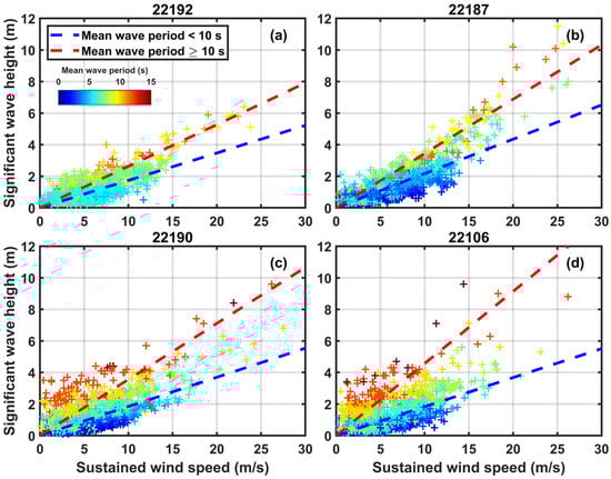
Figure 3.
Comparison between the observed wind speeds and the wave heights at (a) 22192; (b) 22187; (c) 22190; and (d) 22106.
3.2. Validation of Offshore Wind Model Forecasting Data
Figure 4 shows the results of calculating the bias and RMSE by forecast time for all observation points by comparing the offshore wind forecasting data predicted by the Korean Peninsula atmospheric model with the observed data. The bias results by forecast time show a positive bias for the entire forecasting time and indicate the model’s tendency to overestimate (Figure 4a). The forecasting error of RMSE was approximately 2.0 m/s from 0 to 24 h and gradually increased to approximately 3.0 m/s from 24 h to 96 h (Figure 4b). Overall, the forecast error tended to increase as the forecast time increased, but the bias and error range were insignificant. The above results confirmed the atmospheric model’s forecasting accuracy and this study used the offshore wind forecasting data from the Korean Peninsula atmospheric model as the wave model’s input data for all sensitivity numerical simulations.
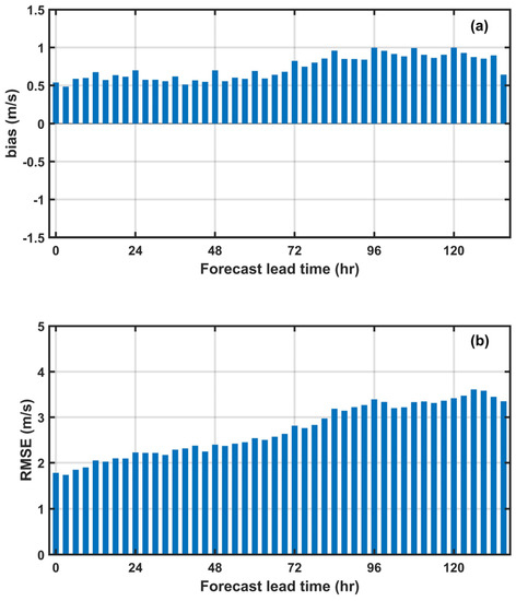
Figure 4.
Validation result of (a) bias and (b) RMSE as a function of lead time for suspended wind speed.
3.3. Wave Model Sensitivity Numerical Simulation Results
The sensitivity test conditions of the wave model were classified according to CDFAC and SINA0, and wave forecasting was performed using the same offshore wind forecasting data. Figure 5 shows the forecasting wind–sea and significant wave height results of the experimental conditions applying CDFAC 1.0 and SINA0 0.05, which were the baseline conditions for the sensitivity numerical simulations in this study. Figure 5a shows the offshore wind and significant wave height at +00 h by running the model at 00 UTC on 4 September 2020. Figure 5b–d show the results at forecast time +24 h, +48 h, and +72 h, respectively. High significant wave heights were forecasted along the trajectory of Typhoon “Haishen”, which occurred in September 2020, indicating that the magnitude and direction of the input wind field directly affect wave development.
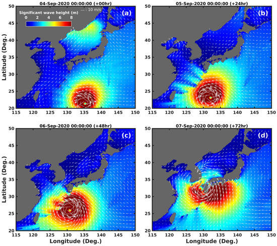
Figure 5.
Numerical simulation result of wind–sea vectors and significant wave height as a function of lead time (a) +00 h; (b) +24 h; (c) +48 h; and (d) +72 h.
In addition to the changes in the input wind field where the atmosphere changes rapidly, such as the occurrences of typhoons, the forecasting results of wave models are also affected by changes in model physical variables related to offshore winds even under general offshore wind conditions. Accordingly, numerical simulation and analysis of sensitivity to physical variables of wave models, such as CDFAC and SINA0, are necessary. Therefore, this study changed the physical variables of the wave model, performed sensitivity numerical experiments on the influential physical variables, and evaluated the forecasting performance under each experimental condition.
Figure 6 shows the observation results at all buoy positions and the wave model’s forecasting results for +24 h. The distribution of significant wave heights is concentrated under 3 m (Figure 6a) and waves appear to develop due to offshore winds of approximately 15 m/s or less (Figure 6b). In terms of the wave period in Figure 6c, most seem to be wind waves of less than 10 s and, as the wave period increases, the model’s tendency to underestimate grows. In particular, the model’s forecasting performance for swell components of 10 s or more was lower than its forecasting performance for wind waves of 10 s or less. In terms of wave direction, the measurements were distributed in the baseline of the observation and model, and the error range was approximately 54° (Figure 6d). The overall forecasting accuracy was high from the input data (offshore wind forecast data). The error analysis results for the significant wave height, wave period, and wave direction predicted by the wave model and the wave model contributed to relatively precise numerical simulations for the correlation between offshore wind and significant wave height. These were the results of analyzing the observation data above.
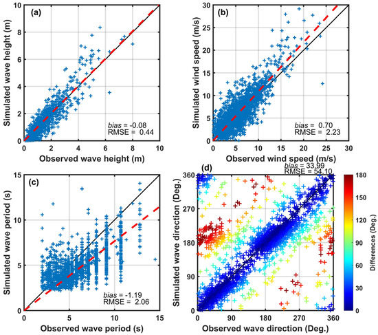
Figure 6.
Comparison between observation and numerical simulation on the forecast lead time +24 h presenting (a) significant wave height; (b) wind speed; (c) wave period; (d) wave direction.
3.4. Impact on Forecasting Performance According to Changes in Wave Model Physical Variables
The model execution period was from 00 UTC on 1 August 2020 to 12 UTC on 30 September 2020. The model was performed twice a day, forecasting up to 120 h. Sensitivity experiments were conducted under the same offshore wind conditions by changing the CDFAC and SINA0 variables. The bias and RMSE for each forecast time were calculated using Equations (9) and (10) for the model forecasting results.
Figure 7 compares the significant wave height time series at +24 h according to CDFAC changes at four buoy points. According to the results of the entire significant wave height time series, the larger the CDFAC, the larger the predicted significant wave height, and the smaller the CDFAC, the smaller the predicted significant wave height. Overall, the time series predicted by the model and the observed time series showed similar trends. However, the significant wave height difference according to CDFAC changes was generally more noticeable when the significant wave height reached its peak value. There was no significant difference when the significant wave height was small.
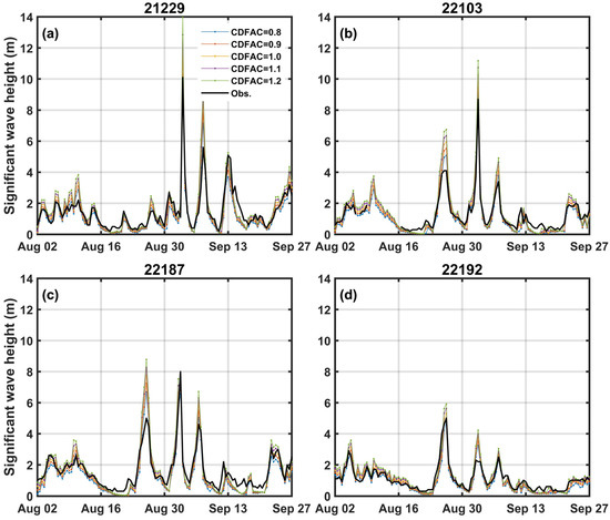
Figure 7.
Comparison of significant wave height changed by CDFAC between observation and numerical simulation on the forecast lead time (+24 h) at (a) 21229; (b) 22103; (c) 22187; (d) 22192.
Figure 8 shows the significant wave height time series according to SINA0 (CDFAC = 1.0) at 22106 and 22190 buoy points. Although SINA0 is a model variable closely related to the direction of the input offshore wind, it was difficult to grasp the effect on the significant wave height forecasting results in the range of SINA0 used in this study. However, in the time series data around 12 September, when the significant wave height was not relatively high and gradually decreased from its peak value, the significant wave height tended to increase when the SINA0 became smaller. When determining the directional distribution in Equation (4), SINA0 is a variable multiplied by adverse winds. Therefore, as the value decreases, the effect of adverse winds becomes relatively small and, as a result, the effect of favorable winds increases. Even if the wind speed is not high, SINA0 can affect the forecasting results in sections where the wind direction changes rapidly by about 180°. However, as it is difficult to grasp the influence of SINA0 on the forecasting results with only the results of this study, we intend to investigate the impact on physical variables in more detail through follow-up studies.
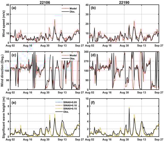
Figure 8.
Relationship between sea–wind condition and significant wave height presenting (a,b) wind speed; (c,d) wind direction; (e,f) significant wave height.
Figure 9 shows the bias and RMSE by forecast time according to CDFAC changes at all observation buoy positions. First, a positive bias was confirmed as the CDFAC increased, and the model’s tendency to overestimate increased (Figure 9a). According to the RMSE by forecast time in Figure 9b, the minimum RMSE was generally shown when the CDFAC range was between 0.8 and 1.1, up to 72 h of the forecast time, and RMSE tended to increase when the CDFAC increased as the forecast time became longer. Figure 10 shows the verification results by forecast time according to SINA0 changes when CDFAC is 1.0. As described above, the bias and RMSE results showed slight differences in only a few sections and did not have a significant effect on the forecasting results in the SINA0 sensitivity test range.
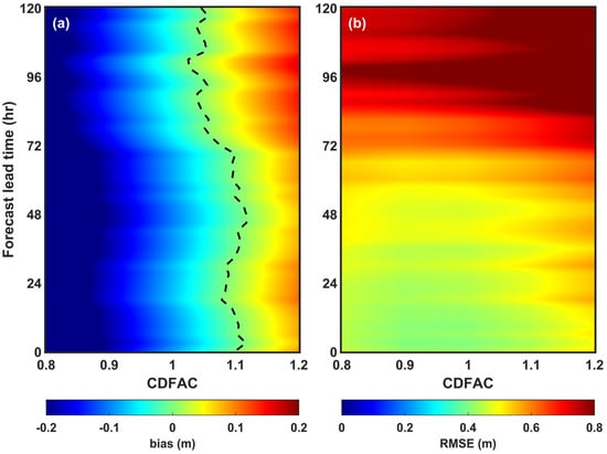
Figure 9.
(a) Bias with equilibrium line (black dot line) and (b) RMSE distributions corresponding to CDFAC changes.
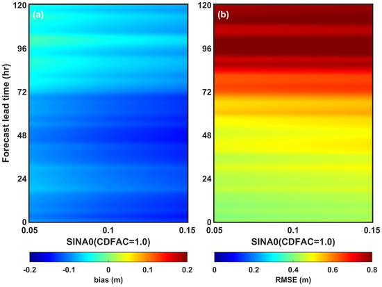
Figure 10.
Validation result of SINA0 changes (CDFAC = 1.0) of (a) bias and (b) RMSE as a function of lead time for significant wave height.
4. Conclusions
This study developed a wave prediction system based on WW3 using offshore wind data from the Korea Integrate Model and performed numerical simulations on the sensitivity of the wave model’s ST6 physics package. Numerical simulations on the sensitivity of the main physical variables were configured to optimize the wave model for forecasting offshore wind data and statistical validation was performed by comparing the model’s forecast results under each experimental condition with observations from marine meteorological buoys.
As a result of analyzing the offshore wind and significant wave height observed from the marine meteorological buoys, the stronger the offshore wind, the higher the wave height. In particular, a relatively high wave height was observed when the wave period was about 10 s or more. This suggests that the relatively high wave height was due to the waves of the swell component rather than the wind wave component. Follow-up studies will be pursued to improve the dynamic structure of the model by analyzing each wave component.
As the forecasting accuracy of a wave model is affected by the offshore wind forecasting accuracy, the quality of the input data must be identified by validating the offshore wind. As a result of comparing the observed offshore wind speed data and the model prediction data, the forecast data of the atmospheric model had a forecast error of about 2 m/s~3 m/s for each forecast time, demonstrating a relatively stable and reliable level of error. Therefore, sensitivity numerical experiments were performed for physical variables CDFAC and SINA0, which, when using the verified offshore wind forecast data, have the most influence on the forecasting performance in the wave model’s ST6 physics package.
The sensitivity numerical experiments were performed by changing the CDFAC, and the effect on wave forecasting was evaluated by changing the SINA0 under the same CDFAC. Although the CDFAC affected the minimum error by forecast time, changing SINA0 under the same CDFAC did not significantly affect the forecast results. However, sections where the wave height rapidly decreased after developing high wave heights tended to maintain a slightly high wave height when the SINA0 was small. This seemed to be due to the directional distribution determined by the sum of adverse and favorable winds in the ST6 physics package. However, it is difficult to confirm this observation, as there are limitations to developing a conclusion based only on the results of this study. Therefore, follow-up studies on the scope and impact of SINA0 will be pursued to investigate this matter.
As described above, the range of variables constituting a wave model’s physics package and their combinations affect the forecasting performance and accuracy of models. Therefore, when constructing a wave prediction system, it is necessary to review the physics package and variables of the model and understand the influence and interaction of physical variables from various angles through sensitivity numerical simulations. Based on the results of this study, we plan to conduct follow-up studies on significant factors that determine the forecasting performance of models. Our objectives will be to improve the forecasting performance and accuracy of wave models and to contribute to providing wave forecast data and live weather information for dangerous weather conditions.
Author Contributions
Conceptualization, M.R. and P.-H.C.; methodology, M.R.; validation, S.-M.O., P.-H.C. and H.-S.K. (Hyung-Suk Kim); formal analysis, M.R.; data curation, M.R. and S.-M.O.; writing—original draft preparation, M.R.; writing—review and editing, M.R.; supervision, H.-S.K. (Hyung-Suk Kim); project administration, H.-S.K. (Hyun-Suk Kang). All authors have read and agreed to the published version of the manuscript.
Funding
This research was funded by the Korea Meteorological Administration Research and Development Program “Development of Marine Meteorology Monitoring and Next-generation Ocean Forecasting System (KMA2018-00420)” and the Basic Science Research Program through the National Research Foundation of Korea (NRF), funded by the Ministry of Education (NRF2021R1A6A1A1A0304518511).
Institutional Review Board Statement
Not applicable.
Informed Consent Statement
Not applicable.
Data Availability Statement
The data and model output that support the findings of this study are available on request from the corresponding author.
Conflicts of Interest
The authors declare no conflict of interest.
References
- Komen, G.J.; Hasselmann, S.; Hasselmann, K. On the Existence of a Fully Developed Wind-Sea Spectrum. J. Phys. Oceanogr. 1984, 14, 1271–1285. [Google Scholar] [CrossRef]
- Tolman, H.L.; Chalikov, D. Source terms in a third-generation wind-wave model. J. Phys. Oceanogr. 1996, 26, 2497–2518. [Google Scholar] [CrossRef]
- Tolman, H.L. Distributed-memory concepts in the wave model WAVEWATCH III. Parallel Comput. 2002, 28, 35–52. [Google Scholar] [CrossRef]
- Ardhuin, F.; Rogers, E.; Babanin, A.V.; Filipot, J.-F.; Magne, R.; Roland, A.; van der Westhuysen, A.; Queffeulou, P.; Lefevre, J.-M.; Aouf, L.; et al. Semiempirical Dissipation Source Functions for Ocean Waves. Part I: Definition, Calibration, and Validation. J. Phys. Oceanogr. 2010, 40, 1917–1941. [Google Scholar] [CrossRef]
- Tsagareli, K.N.; Babanin, A.V.; Walker, D.J.; Young, I.R. Numerical Investigation of Spectral Evolution of Wind Waves. Part I: Wind-Input Source Function. J. Phys. Oceanogr. 2010, 40, 656–666. [Google Scholar] [CrossRef]
- Rogers, W.E.; Babanin, A.V.; Wang, D.W. Observation consistent input and whitecapping dissipation in a model for wind-generated surface waves: Description and simple calculations. J. Atmos. Ocean. Technol. 2012, 29, 1329–1346. [Google Scholar] [CrossRef]
- Ardhuin, F.; Roland, A. The Development of Spectral Wave Models: Coastal and Coupled Aspects. In Proceedings of the 7th International Conference on Coastal Dynamics, Arcachon, France, 23–26 June 2013; Bonneton, P., Garlan, T., Eds.; University of Bordeaux: Bordeaux, France, 2013; pp. 25–38. [Google Scholar]
- Zieger, S.; Babanin, A.V.; Rogers, W.E.; Young, I.R. Observation-based source terms in the third-generation wave model WAVEWATCH. Ocean Model. 2015, 96, 2–25. [Google Scholar] [CrossRef]
- Liu, Q.; Rogers, W.E.; Babanin, A.V.; Young, I.R.; Romero, L.; Zieger, S.; Qiao, F.; Guan, C. Observation-based source terms in the third-generation wave model WAVEWATCH III: Updates and verification. J. Phys. Oceanogr. 2019, 49, 489–517. [Google Scholar] [CrossRef]
- Fan, Y.; Lin, S.J.; Held, I.M.; Yu, Z.; Tolman, H.L. Global ocean surface wave simulation using a coupled atmosphere-wave model. J. Clim. 2012, 25, 6233–6252. [Google Scholar] [CrossRef]
- Chen, S.S.; Zhao, W.; Donelan, M.A.; Tolman, H.L. Directional wind-wave coupling in fully coupled atmosphere-wave-ocean models: Results from CBLAST-Hurricane. J. Atmos. Sci. 2013, 70, 3198–3215. [Google Scholar] [CrossRef]
- Moghimi, S.; Van der Westhuysen, A.; Abdolali, A.; Myers, E.; Vinogradov, S.; Ma, Z.; Liu, F.; Mehra, A.; Kurkowski, N. Development of an ESMF based flexible coupling application of ADCIRC and WAVEWATCH III for high fidelity coastal inundation studies. J. Mar. Sci. Eng. 2020, 8, 308. [Google Scholar] [CrossRef]
- Ortiz-Royero, J.C.; Mercado-Irizarry, A. An intercomparison of Swan and Wavewatch III models with data from NDBC-NOAA Buoys at Oceanic scales. Coast. Eng. J. 2008, 50, 47–73. [Google Scholar] [CrossRef]
- Montoya, R.D.; Osorio Arias, A.; Ortiz Royero, J.C.; Ocampo-Torres, F.J. A wave parameters and directional spectrum analysis for extreme winds. Ocean Eng. 2013, 67, 100–118. [Google Scholar] [CrossRef]
- Barbariol, F.; Alves, J.-H.G.M.; Benetazzo, A.; Bergamasco, F.; Bertotti, L.; Carniel, S.; Cavaleri, L.; Chao, Y.Y.; Chawla, A.; Ricchi, A.; et al. Numerical modeling of space-time wave extremes using WAVEWATCH III. Ocean Dynam. 2017, 67, 535–549. [Google Scholar] [CrossRef]
- Abdolali, A.; Roland, A.; van der Westhuysen, A.; Meixner, J.; Chawla, A.; Hesser, T.J.; Smith, J.M.; Sikiric, M.D. Large-scale hurricane modeling using domain decomposition parallelization and implicit scheme implemented in WAVEWATCH III wave model. Coast. Eng. 2020, 157, 103656. [Google Scholar] [CrossRef]
- Abdolali, A.; van der Westhuysen, A.; Ma, Z.; Mehra, A.; Roland, A.; Moghimi, S. Evaluating the accuracy and uncertainty of atmospheric and wave model hindcasts during severe events using model ensembles. Ocean Dyn. 2021, 71, 217–235. [Google Scholar] [CrossRef]
- Ris, R.C.; Holthuijsen, L.H.; Booij, N. A third-generation wave model for coastal regions: 2. Verification. J. Geophys. Res. 1999, 104, 7667–7681. [Google Scholar] [CrossRef]
- Bi, F.; Song, J.; Wu, K.; Xu, Y. Evaluation of the simulation capability of the Wavewatch III model for Pacific Ocean wave. Acta Oceanol. Sin. 2015, 34, 43–57. [Google Scholar] [CrossRef]
- Zieger, S.; Vinoth, J.; Young, I.R. Joint calibration of multiplatform altimeter measurements of wind speed and wave height over the past 20 years. J. Atmos. Ocean. Technol. 2009, 26, 2549–2564. [Google Scholar] [CrossRef]
- Ponce de León, S.; Bettencourt, J.H. Composite analysis of North Atlantic extra-tropical cyclone waves from satellite altimetry observations. Adv. Space Res. 2021, 68, 762–772. [Google Scholar] [CrossRef]
- Liu, Q.; Babanin, A.V.; Guan, C.; Zieger, S.; Sun, J.; Jia, Y. Calibration and validation of HY-2 altimeter wave height. J. Atmos. Ocean. Technol. 2016, 33, 919–936. [Google Scholar] [CrossRef]
- Campos, R.M.; Alves, J.H.G.M.; Soares, C.G.; Guimaraes, L.G.; Parente, C.E. Extreme wind-wave modeling and analysis in the south Atlantic ocean. Ocean Model. 2018, 124, 75–93. [Google Scholar] [CrossRef]
- Hasselmann, S.; Hasselmann, K.; Allender, J.H.; Barnett, T.P. Computations and parameterizations of the nonlinear energy transfer in a gravity-wave specturm. Part II: Parameterizations of the nonlinear energy transfer for application in wave models. J. Phys. Oceanogr. 1985, 15, 1378–1392. [Google Scholar] [CrossRef]
- Van Vledder, G.P. The WRT method for the computation of non-linear four-wave interactions in discrete spectral wave models. Coast. Eng. 2006, 53, 223–242. [Google Scholar] [CrossRef]
- WAVEWATCH III Development Group, User Manual and System Documentation of WAVEWATCH III Version 6.07. Techn., 333. Available online: https://github.com/NOAA-EMC/WW3/wiki/files/manual.pdf (accessed on 25 January 2023).
- Stopa, J.E. Wind forcing calibration and wave hindcast comparison using multiple reanalysis and merged satellite wind datasets. Ocean Model. 2018, 127, 55–69. [Google Scholar] [CrossRef]
- Campos, R.M.; D’Agostini, A.; Franca, B.R.L.; Damiao, A.L.A.; Soares, C.G. Implementation of a multi-grid operational wave forecast in the South Atlantic Ocean. Ocean Eng. 2022, 243, 110173. [Google Scholar] [CrossRef]
- Moon, I.J.; Ginnis, I.; Hara, T.; Thomas, B. Physics-based parameterization of air-sea momentum flux at high wind speeds and its impact on hurricane intensity predictions. Mon. Weather Rev. 2006, 135, 2869–2878. [Google Scholar] [CrossRef]
- Babanin, A.V.; Banner, M.L.; Young, I.R.; Donelan, M.A. Wave-follower field measurements of the wind-input spectral function. Part III: Parameterization of the wind-input enhancement due to wave breaking. J. Phys. Oceanogr. 2007, 37, 2764–2775. [Google Scholar] [CrossRef]
- Waters, J.; Wyatt, L.R.; Wolf, J.; Hines, A. Data assimilation of partitioned HF radar wave data into Wavewatch III. Ocean Model. 2013, 72, 17–31. [Google Scholar] [CrossRef]
- Qi, P.; Cao, L. Establishment and tests of EnOI assimilation module for WAVEWATCH III. Chin. J. Ocean. Limnol. 2015, 33, 1295–1308. [Google Scholar] [CrossRef]
- Li, J.; Zhang, S. Mitigation of model bias influences on wave data assimilation with multiple assimilation systems using WaveWatch III v5.16 and SWAN v41.20. Geosci. Model Dev. 2020, 13, 1035–1054. [Google Scholar] [CrossRef]
- Li, J.-G. Propagation of ocean surface waves on a spherical multiple-cell grid. J. Comput. Phys. 2012, 231, 8262–8277. [Google Scholar] [CrossRef]
- Amrutha, M.M.; Kumar, V.S.; Sandhya, K.G.; Nair, T.B.; Rathod, J.L. Wave hindcast studies using SWAN nested in WAVEWATCH III—Comparison with measured nearshore buoy data off Karwar, eastern Arabian Sea. Ocean Eng. 2016, 119, 114–124. [Google Scholar] [CrossRef]
- Kuznetsova, A.; Baydakov, G.; Papko, V.; Kandaurov, A.; Vdovin, M.; Sergeev, D.; Troitskaya, Y. Adjusting of Wind Input Source Term in WAVEWATCH III Model for the Middle-Sized Water Body on the Basis of the Field Experiment. Adv. Meteorol. 2016, 2016, 8539127. [Google Scholar] [CrossRef]
- Kazeminezhad, M.H.; Siadatmousavi, S.M. Performance evaluation of WAVEWATCH III model in the Persian Gulf using different wind resources. Ocean Dynam. 2017, 67, 839–855. [Google Scholar] [CrossRef]
- Siadatmousavi, S.M.; Jose, F.; da Silva, G.M. Sensitivity of a third generation wave model to wind and boundary condition sources and model physics: A case study from the South Atlantic Ocean off Brazil coast. Comput. Geosci. 2016, 90, 57–65. [Google Scholar] [CrossRef]
- Fernández, L.; Calvino, C.; Dias, F. Sensitivity analysis of wind input parametrizations in the WAVEWATCH III spectral wave model using the ST6 source term package for Ireland. Appl. Ocean Res. 2021, 115, 102826. [Google Scholar] [CrossRef]
- Kalourazi, M.Y.; Siadatmousavi, S.M.; Yeganeh-Bakhtiary, A.; Jose, F. WAVEWATCH-III source terms evaluation for optimizing hurricane wave modeling: A case study of Hurricane Ivan. Oceanologia 2021, 63, 194–213. [Google Scholar] [CrossRef]
- Roh, M.; La, N.R.; Oh, S.M.; Kang, K.R.; Oh, Y.J.; Kim, H.S. Verification of forecast performance of a rapid refresh wave model based on wind-wave interaction effect. J. Mar. Sci. Eng. 2021, 9, 1230. [Google Scholar] [CrossRef]
- Beyramzadeh, M.; Siadatmousavi, S.M.; Derkani, M.H. Calibration and skill assessment of two input and dissipation parameterizations in WAVEWATCH-III model forced with ERA5 winds with application to Persian Gulf and Gulf of Oman. Ocean Eng. 2021, 219, 108445. [Google Scholar] [CrossRef]
- Shao, W.; Yu, W.; Jiang, X.; Shi, J.; Wei, Y.; Ji, Q. Analysis of Wave Distributions Using the WAVEWATCH-III Model in the Arctic Ocean. J. Ocean Univ. China 2022, 21, 15–27. [Google Scholar] [CrossRef]
- Hwang, P.A. A note on the ocean surface roughness spectrum. J. Atmos. Ocean. Technol. 2011, 28, 436–443. [Google Scholar] [CrossRef]
- WMO. Guide to Wave Analysis and Forecasting, 3rd ed.; World Meteorological Organization (WMO): Geneva, Switzerland, 2018; p. 131. [Google Scholar]


Disclaimer/Publisher’s Note: The statements, opinions and data contained in all publications are solely those of the individual author(s) and contributor(s) and not of MDPI and/or the editor(s). MDPI and/or the editor(s) disclaim responsibility for any injury to people or property resulting from any ideas, methods, instructions or products referred to in the content. |
© 2023 by the authors. Licensee MDPI, Basel, Switzerland. This article is an open access article distributed under the terms and conditions of the Creative Commons Attribution (CC BY) license (https://creativecommons.org/licenses/by/4.0/).