Scenario Analysis of Cost-Effectiveness of Maintenance Strategies for Fixed Tidal Stream Turbines in the Atlantic Ocean

Abstract

This paper has developed an operation and maintenance (O&M) model for projected 20 MW tidal stream farm case studies at two sites in the northeast Atlantic in France and at EMEC’s Fall of Warness site in the UK. The annual energy production, number of incidents, and downtimes of the farms for corrective and planned (preventive) maintenance strategies are estimated using Monte Carlo simulations that vary weather windows, repair vessel availabilities, and mean annual failure rates modelled by Weibull distributions. The trade-offs between the mean annual failure rates, time availability, O&M costs, and energy income minus the variable O&M costs were analysed. For all scenarios, a 5-year planned maintenance strategy could considerably decrease the mean annual failure rates by 37% at both sites and increase the net energy income. Based on a detailed sensitivity analysis, the study has suggested a simple decision-making method that examines how the variation in the mean annual failure rate and changes in spare-part costs would reduce the effectiveness of a preventive maintenance strategy. This work provides insights into the most important parameters that affect the O&M cost of tidal stream turbines and their effect on tidal energy management. The output of the study will contribute to decision-making concerning maintenance strategies.

1. Introduction

The development of offshore and marine energy is essential for global energy decarbonization. It is especially important for countries that have a high import dependency on fossil-based fuel energy while having great potential for marine energy, such as those in Europe.

In 2021 alone, Europe installed 17.4 gigawatts of wind power capacity, according to figures from the industry body Wind Europe. In the European Commission draft strategy [1], the target is to increase the current installed capacity of 12 GW of fixed offshore wind (in 2020) to 60 GW by 2030 and to 300 GW by 2050. In addition, the Commission wishes to have 40 GW of ocean energy (wave and tidal) and other emerging technologies such as floating wind and solar by 2050. The required investment to achieve these targets is estimated at nearly €800 billion between now and 2050.

While there is a great deal of attention paid to the potential of marine energy, the footprint of tidal stream and wave projects remains very small compared to other renewables such as wind. It is expected that tidal stream energy will become fully commercial in the next decade [2]. The cumulative global installed capacity of tidal stream energy from 2010 to 2020 reached nearly 36 MW [3], of which almost 28 MW is in Europe [4]. Many of the tidal stream device developers have gone through the tank testing stage and reached technology level readiness (TRL) 5, and a few of them have achieved TRL 7–9, the full-scale open-sea testing and commercial deployment levels. In [5], the TRLs of the worldwide tidal turbine technologies are listed; Ref. [6] suggests a set of six stages of tidal technology development from concept creation to commercial array demonstration and their links to the TRL 1 to TRL 9 scale.

In the list of recognised tidal stream energy converters, which is presented in Figure 1, the horizontal axis turbine is the most common worldwide technology. This harnesses the kinetic energy of sea currents to generate electricity in the same manner that wind turbines capture energy from the wind [7], but tidal turbines are smaller in size [8]. Horizontal axis turbines are currently in the pre-commercialization to commercialization stage and, compared to other tidal stream energy devices, have a lower annual failure rate [9]. Many companies around the world have developed this technology, including SIMEC Atlantis (UK), ANDRITZ HYDRO Hammerfest (The Netherlands), Verdant Power (US), Magallanes Renovables (Spain), Nova Innovation (UK, Canada), and Sabella (France) [10]. Some projects have been grid-connected. For example, in 2019, MeyGen’s tidal stream array of four turbines exported more than 24 GWh of electricity to the grid. That was enough to power 4000 homes, and MeyGen’s tidal stream array will power 177,000 homes with its 250 turbines in the next phase [11].

Tidal energy converters (TECs) are technically feasible, but the costs associated with their deployment and operation are still highly uncertain [12]. Some studies have investigated the levelized cost of energy (LCoE) of tidal stream energy for case studies. The LCOE of a dual-rotor horizontal-axis tidal turbine was estimated to be $410/MWh (€307/MWh) in the US in 2014 [13]. Catapult Offshore Renewable Energy (OREC) has calculated an LCoE of £300/MWh (approximately €370/MWh) for a 10 MW tidal stream installed in the UK as of 2012. In the technical report by the Joint Research Centre (JRC), a reference LCoE value of €620/MWh was estimated in 2015 [14]. Although the sector has considerably reduced the cost by 40% since 2015 [15], the LCoE is still high compared to that of fixed offshore wind energy at £109/MWh (€123/MWh in 2018) [16]. It has been predicted that the drivers, such as the learning factors, innovations, and reduction of the capital cost, would reduce the LCoE of a 1 GW tidal stream to €100/MWh [17]. However, even at this level of LCoE, tidal energy can hardly compete with emerging floating offshore wind energy. For commercial floating offshore wind (e.g., above 1 GW), the LCoE is currently estimated to be £176/MWh (€211/MWh), reducing to between £83–104/MWh (€100–125/MWh) and with recent predictions of a further reduction to circa £53/MWh (€64/MWh) by 2030 [18].

Operation and Maintenance (O&M) is a significant contributor to the LCoE. For example, for offshore wind energy, the O&M cost could account for around 28% of the LCoE [19]. One of the crucial considerations in the O&M analysis for an offshore renewable energy (ORE) farm is the characterisation of the maintenance vessels [20]. Optimised planning for the operation of vessels like large Service Operation Vessels (SOVs) and Crew Transfer Vessels (CTVs) [21,22,23] can result in reducing the overall maintenance cost. The O&M cost can vary considerably with deployment locations due to distance to port, vessel availability, and the occurrence of weather windows suitable for access [24]. For this reason, several O&M models have been developed, as summarised in [25]. Furthermore, the selection of a suitable maintenance strategy is a key element in reducing the O&M cost and thus the LCoE. For example, by integrating preventive maintenance and condition-based maintenance plans to minimise unplanned (corrective) maintenance costs, it is possible to optimise a project’s economic results [26,27].

A notable difference between the O&M activities of an offshore wind turbine and a tidal stream turbine is that the major O&M activities of tidal turbines will be carried out onshore rather than offshore, meaning that the turbines could be non-operational for longer periods. On the other hand, compared to an offshore wind turbine, a tidal stream turbine is smaller and lighter, meaning that a less complex offshore vessel may be sufficient for maintenance activities. This is the focus of this research. The study uses a dedicated stochastic O&M model developed for tidal stream turbines. The key objective is to provide insights into the parameters with the highest uncertainty associated with the variable O&M activities of projected tidal farms, analysing these through a number of scenarios. The study provides an analysis of the life-time corrective incidents, downtime, and breakdown of the O&M cost components. Furthermore, the study compares the number of failures over the lifetime of the project, the time-based availability, and the value of energy income minus the O&M cost for two maintenance strategies: corrective maintenance (CM) and combined corrective-preventive maintenance (CPM) for a tidal stream farm of 20 MW in two sites in the northeast of the Atlantic Ocean. The quantitative trade-off between the two maintenance strategies is further discussed by changing the annual failure rate input (a very uncertain technical parameter) and spare-part cost (a very uncertain economic parameter) to obtain breakeven where there would be no gain from CPM compared with CM, thus providing a decision support method to show which of CM or CPM is more economically beneficial. The proposed method can be extended to include other maintenance strategies and scenarios that would contribute to the optimisation of O&M strategies that will minimise the LCoE of future tidal farms.

The paper is organised as follows: Section 2 presents the methodology, model description, assumptions, and input data; Section 3 presents the results and discussion; and Section 4 offers the concluding remarks.

2. Methodology

By using the Monte Carlo method [28], a stochastic O&M model was developed to compare two maintenance strategies for a projected tidal farm consisting of 10 × 2 MW turbines at two sites in the northeast Atlantic: France and the UK. In the Monte Carlo simulation, stochastic calculations account for weather windows, vessel availability [18,21], and time between failures [29]. An overview of the model and the processing logic is summarised in Figure 2 and explained further below.

The model in Figure 2 requires substantial input data, including the annual failure rate of tidal components, repair times, vessel characteristics, technician costs, tidal device specifications, electricity loss considerations (e.g., due to the wake and transmission), grid electricity rate, and site specification data (e.g., metocean data, water depth, distance to the facility port). In addition, factors affecting the maintenance activities, such as weather windows (e.g., significant wave height limits for vessel operations) and spare part costs for both maintenance strategies (CM and CPM), need to be determined. Part of the data is obtained from industry, and part is obtained from the literature. The logic of the O&M model is described below, and the remaining part of this section explains the main input data, assumptions, and calculations used to verify the model outcome.

The model generates failure times and calculates downtime in the following steps, as described in

Table 1. Sequence of generating failure times and calculating downtime.

Steps	Brief Description
1. Calculate Weibull parameters for each component using the annual failure rate.	A Weibull distribution is used to simulate the time between failures for the components as described in Section 2.3.1. The mean time between failures is the reciprocal of the annual failure rate.
2. Randomly select the failure time.	Using the Weibull distribution, a random time since the previous failure is selected (or the random time since the component was first used).
3. Calculate the weather window waiting time.	The length of time to repair the component (see Table 2) and the travel time to and from its site (see Table 3) are all known. With this information, the Metocean data is searched to find a weather window that has acceptable wave height and wind speed for the vessel(s) that are needed for repair/maintenance. The start time for this weather window is set to 8 a.m. so that journeys will be made in daylight. It is assumed that weather forecasting is accurate enough to find the weather window. Knowing the waiting time for a weather window and the time required to mobilise the vessel(s), it is then possible to order a vessel to arrive at the start of the weather window.
4. Retrieve the turbine offshore, return the turbine to the facility port, carry out (onshore) repair, decide to hold on to the vessel(s) or re-hire them when the turbine is returned to function in the farm, and calculate the downtime.	Calculate the time for the journey to and from the farm, the time to retrieve and re-install the device offshore (see Table 3), and the time to repair it onshore (Table 2). The decision then is whether to keep the vessel on site while the repair is carried out or to send the vessel(s) back and re-hire them. The criterion for this is to decide whether the hiring cost of the time spent waiting for the repair to be completed and the waiting time for the next weather window is more expensive or less expensive than the mobilisation cost of the vessel(s). When the turbine is returned to operation on the farm, this ends the downtime. During downtime, there is a 100% loss of power.
5. Repeat steps 2, 3, and 4 until the project’s lifetime is complete.	The process of repeated repair is continued until the sum of the elapsed time exceeds the lifetime of the project.

.

In addition to corrective maintenance, planned maintenance is scheduled at five-year intervals. Planned maintenance is carried out in the summer when the weather window is almost nil or minimal (see Section 2.4 for a description of the weather window). It is assumed that the port facility has enough space for 10 turbines, and the planned maintenance will be performed without any delay. For each turbine, on average, 8 technicians (working a 12 h shift) will carry out the planned maintenance task over 220 h (i.e., 18.3 days).

Planned maintenance will increase the reliability of the turbine [26]. Regular maintenance activities can reduce the likelihood of component failure. This study has considered that after the planned maintenance, the turbine is as good as a one-year-old device. This will minimise the degradation of components and, therefore, reduce their failure occurrence. In other words, it increases the time between failures.

The spare part cost per turbine for planned maintenance is assumed to be, on average, around 2% of the price of the tidal turbine device. A tidal turbine (per MW) is more expensive than a wind turbine due to its environment. The CAPEX/MW (including device cost, installation, and foundation) of a horizontal tidal stream turbine could range between 2.3–4 £/MW, which is higher by a factor of around 1.1–1.5 compared to a (fixed) offshore wind turbine [24]. The cost of the foundation and installation could account for around 32% of the total CAPEX, meaning that the cost of a tidal turbine device could range between 1.6 €m/MW and 2.7 €m/MW (on average 2.2 €m/MW). On this basis, it is assumed that a commercial 2 MW tidal stream turbine would cost circa 4 €m. Therefore, the average cost of spare parts used for planned maintenance will be €80,000 per turbine (€12,800 on average over the whole life of the project per year per turbine). Through sensitivity analysis, the upper limits of spare part costs that would make preventive maintenance a cost-effective option are discussed in Section 3.1.

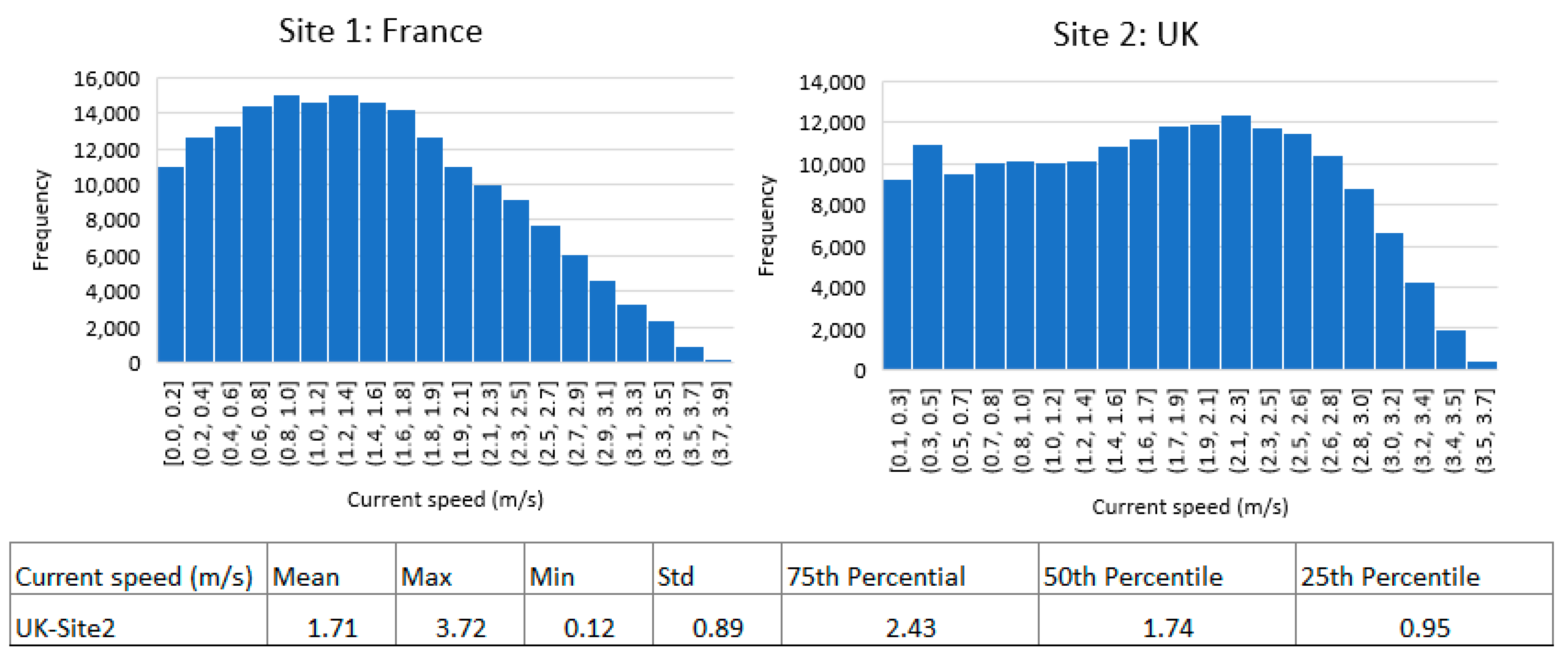
2.1. Site-Specific Weather Condition Statistics

The time-series metocean data of the two locations in the northeast Atlantic Ocean: Site1 in France and Site2 in the Fall of Warness were obtained from industry. Twenty-five-year hourly metocean data for these two sites has been used for the project life-time of an array of 20 MW (10 tidal turbines of 2 MW each) in the model. The characteristics of the tidal device are explained in the next sub-section. The statistics of the current speed and the weather window data for the two sites are briefly explained below. Histograms and statistics of measured current velocities at a water depth of 35 m below the surface for Site1 (France) and 42 m for Site2 (UK) over 25 years are shown in Figure 3.

Both the mean and median (50th percentile) of the UK site, which are approximately 1.7 m/s, are bigger than those for the French site.

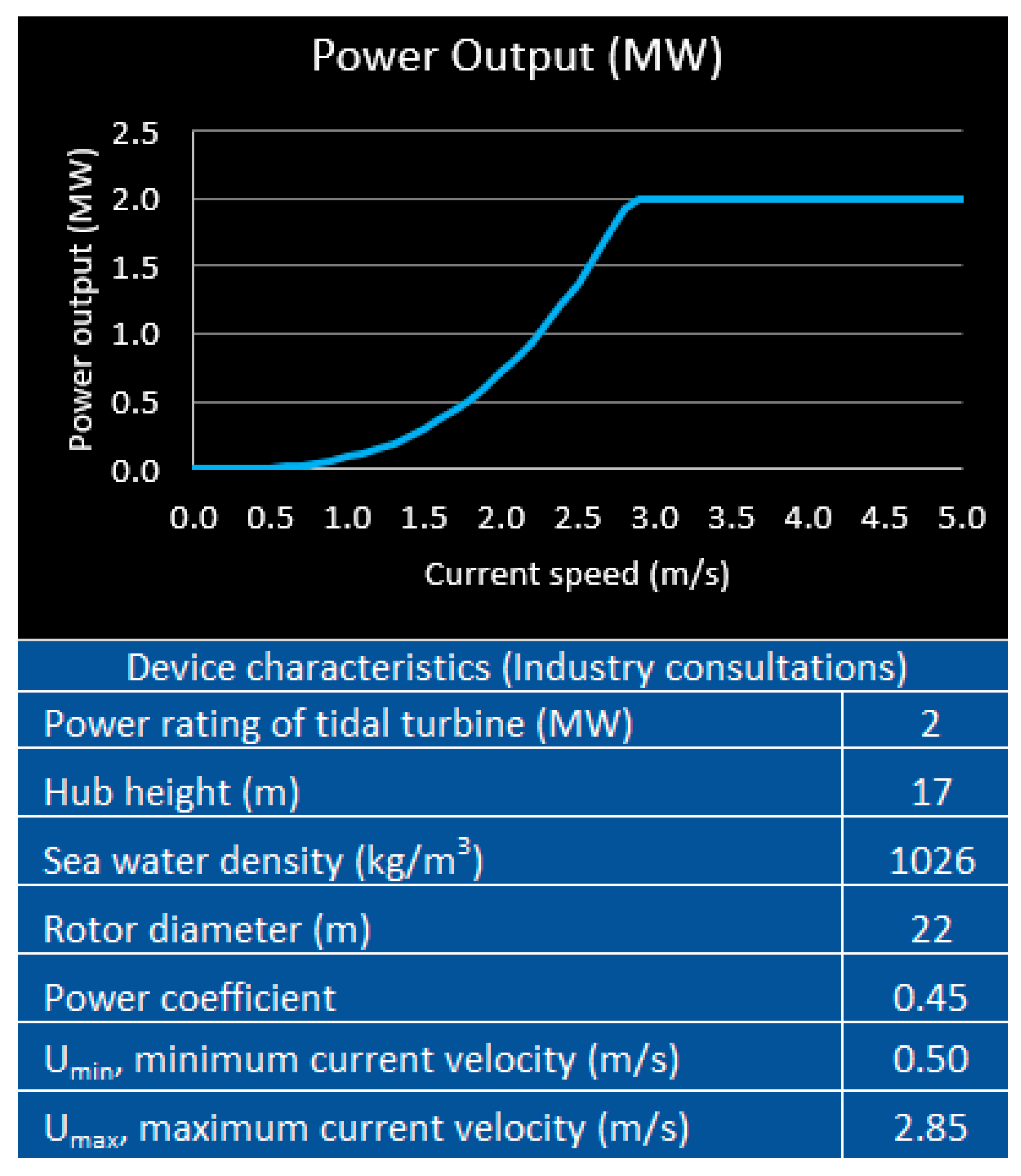
2.2. Tidal Device Specification and Energy Production

Horizontal-axis tidal stream turbines similar to Sabella have been considered in the model. Sabella has developed an expansive range of turbines from 100 kW to 2 MW, and for the purpose of scenario analysis, this paper has considered fixed 2 MW tidal turbines. The following key sub-assemblies make up the turbine:

• Rotor blades, which capture the kinetic energy of the moving water.
• Hub, the central part of the turbine that connects the rotor blades to the generator. It typically consists of a hub housing and a shaft.
• Generator, which is responsible for converting the mechanical energy of the rotating rotor into electrical energy. It is typically located inside the nacelle, which is mounted on top of the tower.
• Control system, which monitors and regulates the operation of the turbine, including the speed of the rotor and the output of the generator. It may also include sensors to monitor environmental conditions such as tidal currents, water depth, and temperature.
• Power transmission system, which is responsible for transmitting the electrical energy generated by the turbine to the shore. It typically consists of underwater cables, a substation, and a connection to the grid.
• A ballast-weight foundation that provides a stable base for the turbine.

Using the assumed parameters of the turbine and power curve shown in Figure 4 that were determined through industry consultations, the model calculates the expected (theoretical) power production from the turbine, which is explained below.

The rated power for the rotor occurs at a current speed of about 2.85 m/s, as shown in the power curve in Figure 4. For tidal energy, power is proportional to the cube of the volumetrically averaged current velocity over the rotor swept area, the turbine power coefficient, and the sea water density [2]. The theoretical annual energy production in MWh is calculated through Equation (1):

$$\begin{array}{l}\mathit{For} 0\le u_t<u_{\mathit{min}}, P_t=0;\\ \mathit{For} u_{\mathit{min}}\le u_t<u_{\mathit{max}},P_t=(0.5) C_p\rho A{\left(u_t\right)}^3/1000;\\ \mathit{For} u_t\ge u_{\mathit{max}},P_t=(0.5) C_p\rho A{\left(u_t\right)}^3/1000,\\ \mathit{Theoretical} \mathit{annual} \mathit{energy} \mathit{in} \mathit{MWh}={\sum }_{t=1}^{8760}{P}_t,\end{array}$$

(1)

where, P_t is the power generated at hour t, u_t is the current velocity (adjusted at the hub height) in m/s at hour t, u_min is the minimum velocity captured by the device in m/s, u_max is the maximum velocity captured by the device in m/s, C_p is the power co-efficient, A is the rotor swept area in m² (i.e., the rotor radius squared times 3.14), and ρ is the sea water density in kg/m³ (Figure 4). Note that the sum for leap years is taken over the period of 8784 h. The current velocity (u_t) at the level of hub height is extrapolated from the velocity at measurement height (i.e., 35 m for Site1 and 42 m for Site2 as mentioned in Section 2.1) up to the device hub height (i.e., 17 m as shown in Figure 4) using the 1/7th (i.e., 0.14) power law exponent [30,31].

The annual energy production (AEP) of the farm was calculated after including the possible losses, e.g., losses due to the wake and electricity transmission. Tidal devices will alter the drag coefficient and flow pattern of the site. This effect could result in reducing the power extraction of the other tidal turbines if they are arranged in a typical farm configuration and will necessitate the careful tuning of individual turbines to achieve optimal output [32,33]. Several studies have investigated the effect of downstream wake (i.e., velocity deficit), for example, [32,33,34,35,36]. Very close lateral spacing between turbines would cause a large velocity deficit downstream and therefore a significant decrease in the available power for downstream turbines [35]. The influence of downstream wake effects on the AEP could be as high as 10% to 20% [3]. Ref. [34] suggests that at the lateral spacing of 7D (seven times the rotor diameter), the velocity deficit would be insignificant. Inter-row spacing is not the only concern, as there is a strong effect in the direction of the tidal flow, which can reduce the energy output of the back turbines by up to 30% compared to those at the front [36]. An optimal layout of the tidal devices, for example, a staggered configuration with small rows of devices, minimises the wake effect losses of the last rows and therefore improves the total energy captured by the tidal farm [37]. The electricity transmission loss depends on the type of transmission system and cable export distance. For example, the study by [38] suggests an average total power loss of around 2.5% for a cable distance of 50 km. This study has assumed an average loss of 5% due to downstream wake loss and 3% due to electricity transmission loss. Considering these losses, the AEP will be calculated as:

AEP (MWh) = Theoretical Power (MWh) × (1 − 0.05) × (1 −0.03)

(2)

The annual income from selling the electricity to the grid will be calculated by multiplying the delivered energy, after including downtime due to the weather window and time to repair, by the grid rate of 200 €/MWh considered in the study.

2.3. Failure Data Input

In the model, failure means that a part of the tidal device or a component faces an unplanned interruption, resulting in the failed operation of the device [9]. The annual failure rates of the tidal device components, the mean time to repair, the approximate cost of the spare part, and the required number of technicians were obtained through industry consultations. All repairs are carried out at on-shore port facilities, which are within 15 km of the farm site. The failure data on a component-by-component basis are presented in

Table 2. Failure data for each component along with the repair data input for one device.

Component	Annual Failure Rate (%)	Time to Repair (h)	Spare-Part Cost €	No. of Technicians
Drivetrain	44	60	45,000	4
Electric system	17	5	3500	2
Nacelle	12	60	35,000	6
Blade	9	7	2500	2
Support structure	6	500	200,000	8
Pitch system	4	44	8000	4
Gearbox	4	45	70,000	4
Power convertor	2	50	15,000	4
Generator	2	140	25,000	4
Control system	1	45	4000	2
Sum	100	956	408,000	40

. In order to protect the commercially sensitive data of the annual failure rates that were provided by the industry, this data is aggregated and normalised in Table 2. Drivetrain failures are the most frequent failures, followed by electric system, nacelle, and blade component failures. For components with major and minor annual failure rates provided by the industry, only the major annual failure rates are considered. The failures in Table 2 are all major failures, except the failures of ‘electric system’ and ‘blade’ components, which are minor. For both CM and CPM strategies, a 12 h shift for technicians is considered, and the average hourly cost of one technician is €50.

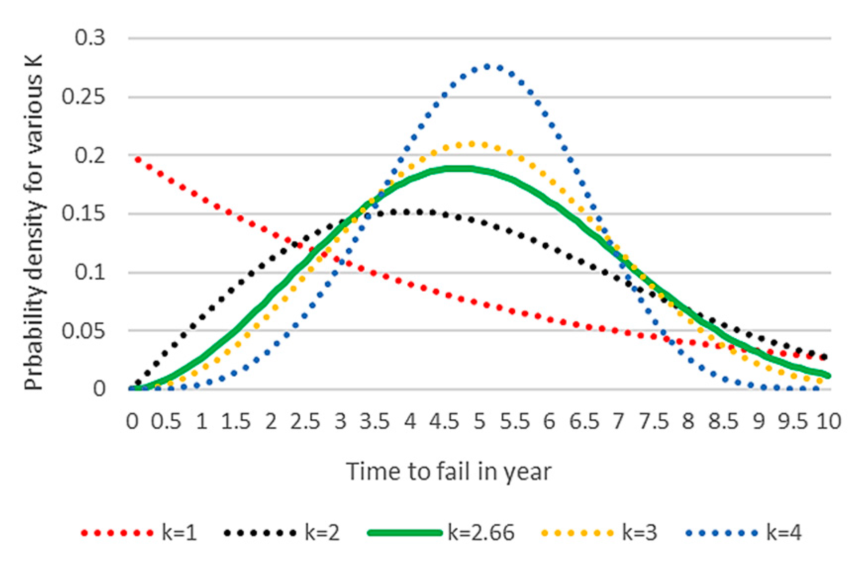
2.3.1. Failure Event Distribution

Although failure rates are frequently discussed in the literature, it is the time between failures that is the subject of the statistical modelling used here and in the literature. The failure rate is used to calculate the mean time between failures; the lengths of time between failures are random events that can be usefully modelled using a distribution.

While exponential distribution is often used to model the time between failures, this usage assumes that failure events are the result of a purely random Poisson process. In the case of mechanical equipment failure, a credible cause of failure is wear and tear; therefore, the age of a component is a key driver of failure. This gives the choice of several distributions, notably Weibull, Lognormal, and Gamma, which simulate positive values without an upper limit.

The Gamma distribution is useful to model events that are not completely random, such as the time until the nth occurrence of a Poisson process; however, this does not give sufficient weight to the effect of wear and tear on mechanical components as is required for this study. The choice between Lognormal and Weibull is based on their respective hazard functions and the preferences seen in the literature. The hazard function of a Weibull distribution with a shape parameter k > 1, which is the case for wear and tear modelling, increases with age, while the hazard function of a Lognormal distribution reaches a peak and declines with age [39]. Therefore, since wear and tear only increases with age, this indicates a preference for Weibull. There is some research suggesting that there may be little to choose between Lognormal and Weibull for situations with sparse data [40,41], but given the preference for Weibull in the literature for modelling reliability and failure analyses of wind turbines, for examples see [42,43,44], the Weibull distribution was selected for this study.

As mentioned earlier, the study uses Monte Carlo simulations [28] to consider the impact of inherently uncertain or stochastic variables on the model’s results. In the CM strategy, the primary stochastic variable modelled for each component is the length of time until a failure occurs (for a new component) or the time between failures (for a repaired component). For each iteration, the time to failure is modelled as a random selection from a Weibull distribution [45,46], where the parameters k and lambda ($\lambda )$, respectively known as the shape and scale, are calculated based on the mean annual rate of failure and the reasonable assumption that there is a 1% probability that a component will fail before one fifth of its mean time between failures. This assumption is based on the behaviour of mechanical devices, where failure of a new component is less likely than failure of an older component due to wear and tear. The choice of the shape parameter produced by this assumption, shown in Figure 5 (solid green line), k = 2.66, is in line with the literature, for example [47]. This value for the shape parameter k may be found using Equations (1) and (2) [48] with the Weibull cumulative distribution function, CDF = 0.99, and the Weibull Mean Time Between Failure (MTBF) divided by five replacing x. The following pair of equations for k are solved numerically.

$$CDF=1-e^{-{\left(\frac{x}{\lambda }\right)}^k}$$

(3)

$$MTBF=\lambda \Gamma \left(1+\frac{1}{k}\right)$$

(4)

In Figure 5, the PDF function for several values of the shape parameter k is displayed, and it is seen that for k > 1, there is a lower probability of failure soon after the component is new but a higher probability later reaching a maximum and then decreasing. The probability decreases after the maximum because of the lower likelihood that a component will last a very long time. For the case of k = 1, the exponential distribution, the probability of failure is at its highest when the component is new and gradually decreases; this does not describe failure due to wear and tear but rather purely random failures perhaps due to outside events such as lightning strikes. In Figure 5, for all of the values of k, the expected value of x, the mean time between failures, is fixed at 5 years.

The failure and repair processes are modelled by repeatedly selecting the time to failure from the Weibull distribution. This process is repeated until the sum of the failures exceeds the total project lifetime (i.e., 25 years). This creates a list of failures that will occur to each component throughout the project lifecycle that will be processed during the simulation. Based on the above methodology, failures will occur at different times for each iteration. This will have an impact on maintenance activities, downtime, and ultimately costs.

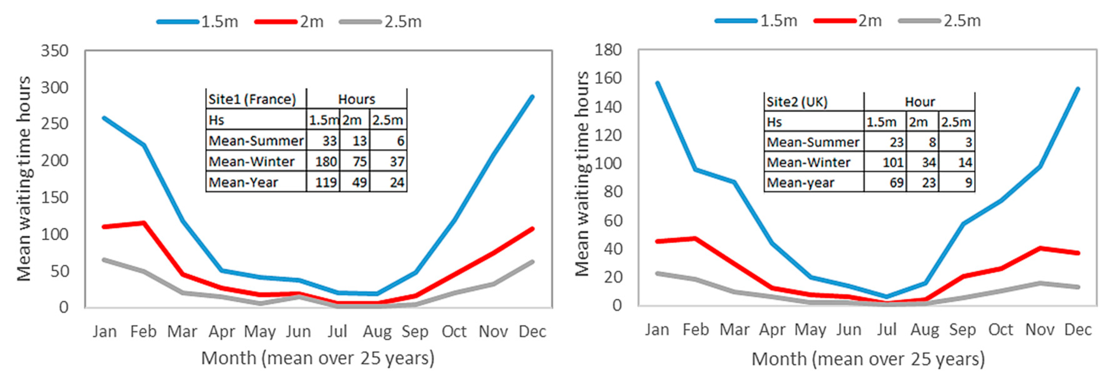
2.4. Weather Window Limit, Vessel Transit Time, and Costs

Weather windows are of particular importance to the O&M cost as they affect the availability of turbines due to waiting time for vessel operations at sea [26]. The current velocity and the weather, specifically wind speed, significant wave height, and wave period, can affect vessel operations, for example, lifting operations and vessel movements [49]. In this model, weather window waiting times are calculated by counting, for each hour of the project life-time, how long it will take until there will be a suitable continuous period for the vessel operations, during which the significant wave height (Hs) and wind speed are within the vessels’ limitations. Graphs illustrating the mean waiting times for Hs ≤ 1.5 m, Hs ≤ 2 m, and Hs ≤ 2.5 m (with wind speed ≤ 20 m/s in all cases) for the two locations and a 24 h weather window gap are shown in Figure 6.

In the study, a multipurpose vessel equipped with a dynamic position system and a 250 t crane is considered in both the CM and CPM strategies. The Hs of 2.5–3 m and wind speed of 20 m/s have been specified for this vessel’s operation. The specifications of the vessel and a summary of the main parameters for calculating the vessel cost are summarised in

Table 3. Vessel characteristics and information on vessel cost calculations.

Dynamic Positioning (DP) Multipurpose	Unit	Value
Average speed (1 knot ≈ 1.852 km/h)	knots	6
Average fuel consumption (transit)	l/hr	596
Average fuel consumption (standby)	l/hr	448
Average fuel price	€/l	0.48
Mobilisation cost	€	50,000
Mobilisation time	hour	48
Operational day rate	€/day	40,000
Retrieving time of the device (offshore)	hr	6
Reinstallation time of the device (offshore)	hr	6
A summary of vessel cost calculations
(i) Transit time (hr) = Distance from port in km/vessel speed in km per hour
(ii) Total vessel use time (hr) = Retrieving time + Reinstallation time +Transit time ×4
(iii) Vessel fuel cost (€) = Total vessel use time (hr) × Fuel consumption (l/hr) × Fuel price (€/l)
(iv) Vessel operation cost (€) = Total vessel use time (in whole number of days) × Vessel operation rate (€/day) + Mobilisation cost

.

Only one maintenance task will be completed per vessel, i.e., the vessel completes a task and returns to the shore before the next task is undertaken. Once it completes a repair/maintenance operation, the vessel becomes available again for the next task.

3. Results and Discussion

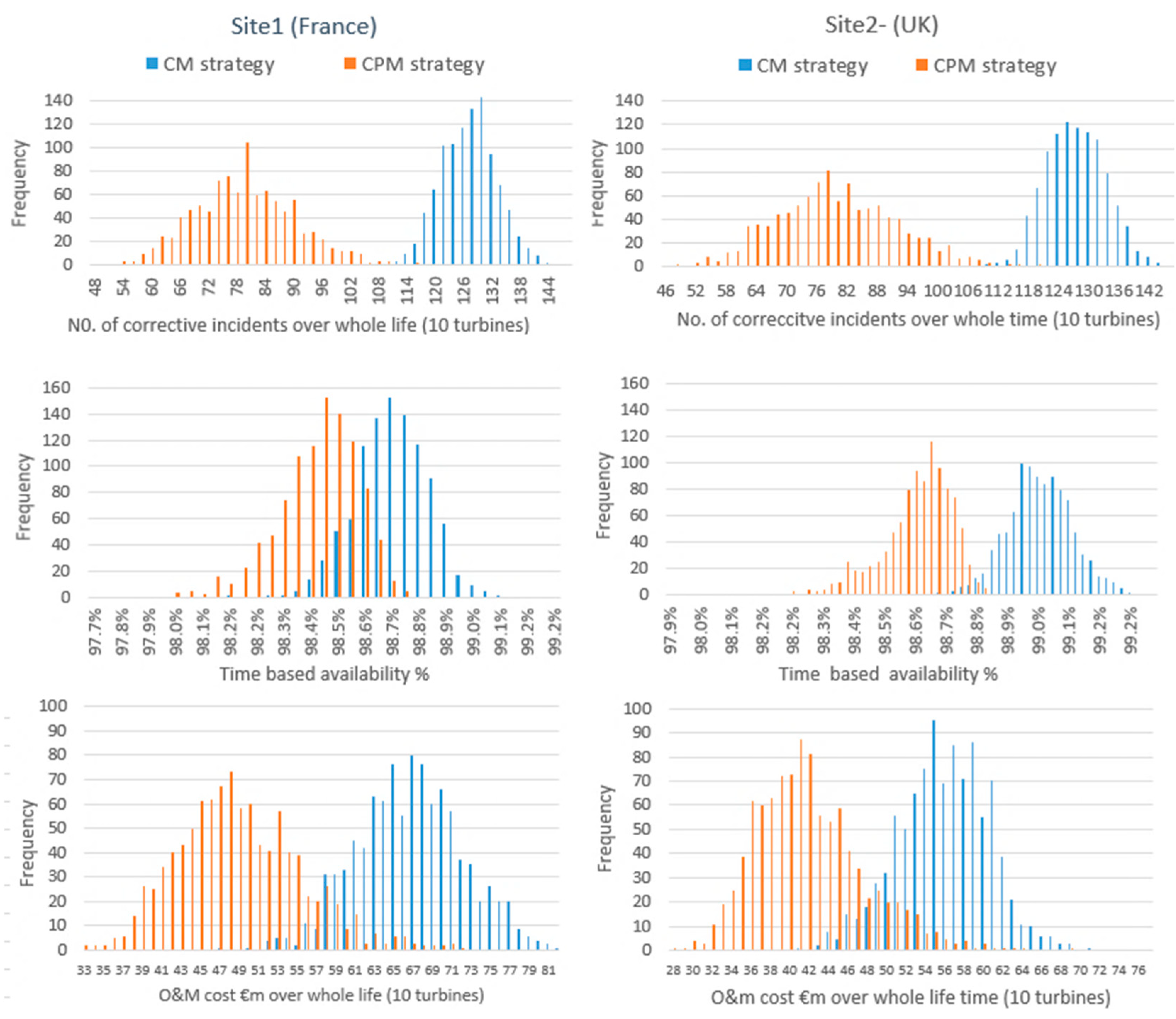
3.1. O&M Metrics and Discussion

A summary of the trade-offs between the two maintenance strategies, as well as the mean annual breakdown of the O&M costs for a turbine located in France (Site1) and the UK (Site2), are presented in

Table 4. Summary of the mean annual O&M parameters.

	CM Strategy		CPM Strategy		Advantage (CPM-CM)/CM
Annual Mean Per Turbine	Site1 France	Site2 UK	Site1 France	Site2 UK	Site1 France	Site2 UK
Number of corrective incidents	0.51	0.51	0.32	0.32	−37%	−37%
Time-based availability	98.7%	99.0%	98.5%	98.6%	−0.2%	−0.4%
Downtime hour	114	88	131	123	−0.2%	−0.4%
Theoretical energy (MWh)	3840	5130	3840	5130	-	-
Delivered energy (MWh)	3482	4665	3476	4651	−0.2%	−0.3%
Gross Income (€)	696,413	932,910	695,143	930,276	−0.2%	−0.3%
Vessel cost (chartered and fuel) (€)	239,203	195,768	154,784	126,451	−35%	−35%
Spare-part cost (€)	20,386	20,427	25,452	25,506	25%	25%
Cost of technicians	9507	9529	17,984	18,015	89%	89%
Annual variable O&M cost (€/turbine/year)	269,096	225,724	198,221	169,972	−26%	−25%
Net income (€/turbine/year)	427,317	707,186	496,922	760,304	16%	7.5%

. The values in Table 4 represent the means of one thousand Monte Carlo simulations over the life-time of 20 MW tidal farms in two locations; the figures are given for one turbine.

Results in Table 4 support the importance of the location on the energy production of ocean energy [3,50]. The table shows that the energy potential for a tidal turbine at the UK location might be around 34% larger than the energy potential for the identical turbine at the France location. This is a result of the higher average current velocity at the UK site than at the French site (see Figure 3). However, it is worth discussing the energy yield with respect to the capacity factor of the device. The average gross capacity factors of the farm are 0.22 in France and 0.29 in the UK site (calculated by dividing the theoretical power production, in Table 4, by the maximum rated power output). The gross capacity factors include energy losses but exclude availability [51]. These factors are relatively low compared to the gross capacity factor of 0.41 of the MeyGen (4 × 1.5) MW project [52] and also compared to the capacity factor of 35% to 40% according to the estimates made by the Ocean Energy System (OES) [51]. The low-capacity factors of the case studies may suggest that the size of the tidal turbine needs to be optimised for the power curve of the device and the deployment locations. Future research would be useful in this regard. Ref. [53] discusses the benefit of the small horizontal tidal stream device (e.g., ≤1 MW) in reducing Capital Expenditure (CAPEX), but more critically, the O&M costs.

With respect to the availability outputs in Table 4, it is clear that for these case studies, the impact of weather conditions on project availability is relatively minimal. The primary reason for this is the model’s employment of an expensive DP vessel with high accessibility (Hs ≤ 3 m and wind speed 20 m/s). It can be seen in Figure 6 that the weather window waiting time for Hs of 2 m, even if a failure occurs in wintertime, is not significant in either of the study locations. However, the figure shows that the availability of the French site is more sensitive to weather conditions. This implies that the reduction in unexpected corrective interventions would be more beneficial in terms of availability and, consequently, energy revenues at the French site compared to the UK site. This is further explained when the CM and CPM results are discussed in this section.

The failures of components in this study do not depend on the deployment sites. Thus, the number of corrective incidents per turbine in Table 4 is seen to be the same in both locations. In the case study, the direct time to repair is around 45 h per turbine per year. This suggests that from the downtime in Table 4, the weather window could account for only 0.8% and 0.5% of the turbine’s availability in the France and UK sites, respectively.

For the CM strategy scenario, the results show that the variable O&M cost of the tidal farm could be 77.3 €/MWh in Site1 (France) and 48.4 €/MWh in Site2 (UK). By considering a five-year-interval planned maintenance strategy, the O&M cost would reduce to 57.0 €/MWh in Site1 (France) and 36.5 €/MWh in Site2 (UK). This considerable reduction in the overall O&M cost for the CPM strategy is due to the 37% reduction in the turbines’ failure rates, which thus reduces the expenses associated with repairs, specifically the vessel costs. In the CPM strategy, the increased cost of spare parts (25%) and technicians (89%) is balanced with the decreased vessel costs (35%). Consistent with other studies, the vessel cost is the dominant component of the O&M cost (for examples, see [29,37]). The vessel cost in this study accounts for more than 84% of the variable O&M cost in the CM strategy and around 72% in the CPM strategy (see Figure 7).

While a CPM strategy greatly reduces the number of corrective incidents that must be dealt with, it also increases the uncertainty as to the corrective incidents. For example, in a ten-turbine array over 25 years, the central 90% confidence interval (CI) for CM strategy is between 120 and 136 incidents (i.e., a width of 16), but the CPM 90% CI is between 66 and 94 (i.e., a width of 30). This is illustrated in the histograms of the numbers of corrective incidents from 1000 simulations in the two top histograms in Figure 8. The histograms of the time-based availability and the total O&M costs for the two strategies are also shown in Figure 8. For example, for the O&M cost, the graph shows that for the majority of simulations of the model, the CPM strategy results in lower O&M costs. There is a region of overlap, indicating that the highest cost outcomes for the CPM strategy can match the lowest cost outcomes of the CM strategy. This also illustrates that the O&M cost depends on non-deterministic factors, such as if and when failures occur.

In order to measure the difference between the two strategies, the financial advantage of a CPM strategy compared with a CM strategy can be expressed as:

$$\begin{gathered} Percentage financial advantage of CPM strategy= \\ \frac{\left(Income-O\&M cost\right) of CPM}{\left(Income-O\&M cost\right) of CM}-1\times 100 \end{gathered}$$

(5)

On average, the financial advantage of a CPM strategy over a CM strategy would be 16.3% in Site1 (France) and 7.5% in Site2 (UK). For both sites, the same number of hours are used for the preventative maintenance operations (i.e., 18.3 days for onshore maintenance tasks plus 1.7 days for transit and retrieval/reinstallation for each turbine), thus reducing the operational time (see the slight change in the time-based availability in Table 4). As a consequence of the preventative maintenance, the failure rates reduce at both sites by the same amount; however, since the weather window waiting time is longer at Site1 (France), there is a greater benefit in terms of operational time and financial advantage compared with Site2. This distinction between the two sites shows the importance of weather window waiting times for Offshore Renewable Energy (ORE) projects.

The histogram of net energy income (i.e., energy income minus O&M cost) in Figure 9 shows that for most of the simulations, the net energy income is higher for the CPM strategy. There is, however, some uncertainty with these types of outcomes as they depend on the random nature of failure events, and so there is an overlap between the worst outcomes of the CPM strategy and the best outcomes of the CM strategy. However, the expected average outcome for CPM is much better in terms of net income than for CM.

The evaluated O&M metrics, namely the Operation Expenditure (OPEX) and availability, of the optimal case study in two locations (CPM strategy) are compared with the earlier work by the Ocean Energy System (OES) in

Table 5. Comparison of the quantified metrics.

Metrics	This Study		Minimum [51]	Maximum [51]
	UK Site	France Site
OPEX 1 €/MWh	50.1	78.1	23.2	102.9
Availability %	98.6	98.5	92.0	98.0

¹ For the OPEX of case studies, 37% is added to the variable O&M cost.

. The OES’s minimum and maximum limits for these measurements are predicated on an initial deployment of 3–90 MW commercial-scale generic horizontal axis tidal stream turbines expected in 2030. The capacity factor of 0.35 in [51] and an exchange rate of 0.902 US$ (2015) are used to convert OPEX in [51] to €/MWh. Since the objective of this study was to address the uncertainty of variable O&M parameters of tidal projects, the other OPEX components, such as insurance, contingency, etc., are educated estimations based on the literature. According to the offshore wind cost reviews by the National Renewable Energy Laboratory (NREL) [54], 63% of OPEX is accounted for by maintenance costs, and the remaining portion (37%) is made up of other operational costs. Assuming that the OPEX split of tidal turbines is the same as fixed offshore wind, the OPEX of the case studies is estimated as shown in Table 5.

The comparison of the measured metrics in Table 5 makes it plainly evident that the study’s OPEX is very close to the highest OES estimations. As was already indicated, the case study’s high OPEX in €/MWh can be attributed to much lower capacity factors, which led to poorer energy yields (despite high availability) than the OES predictions. The requirement for DP vessels (fitted with a crane) to retrieve the tidal device when repair is necessary is another issue that was previously highlighted. Deploying a small fixed tidal turbine size of, e.g., ≤1 MW may require a smaller DP and hence a less expensive vessel. If the deployment of floating devices is assumed, small tugboats, for example, can be used for maintenance tasks on floating tidal turbines, which lowers the OPEX but may have a high upfront CAPEX [54]. In fact, every assumption and input in the model has an impact on O&M costs, prompting a thorough sensitivity analysis in subsequent work. However, given the scope of this study, in addition to the uncertainty analyses of the O&M costs, number of incidents, and availability in Figure 8, a sensitivity analysis is conducted to look into the CPM strategy’s benefits in the following section.

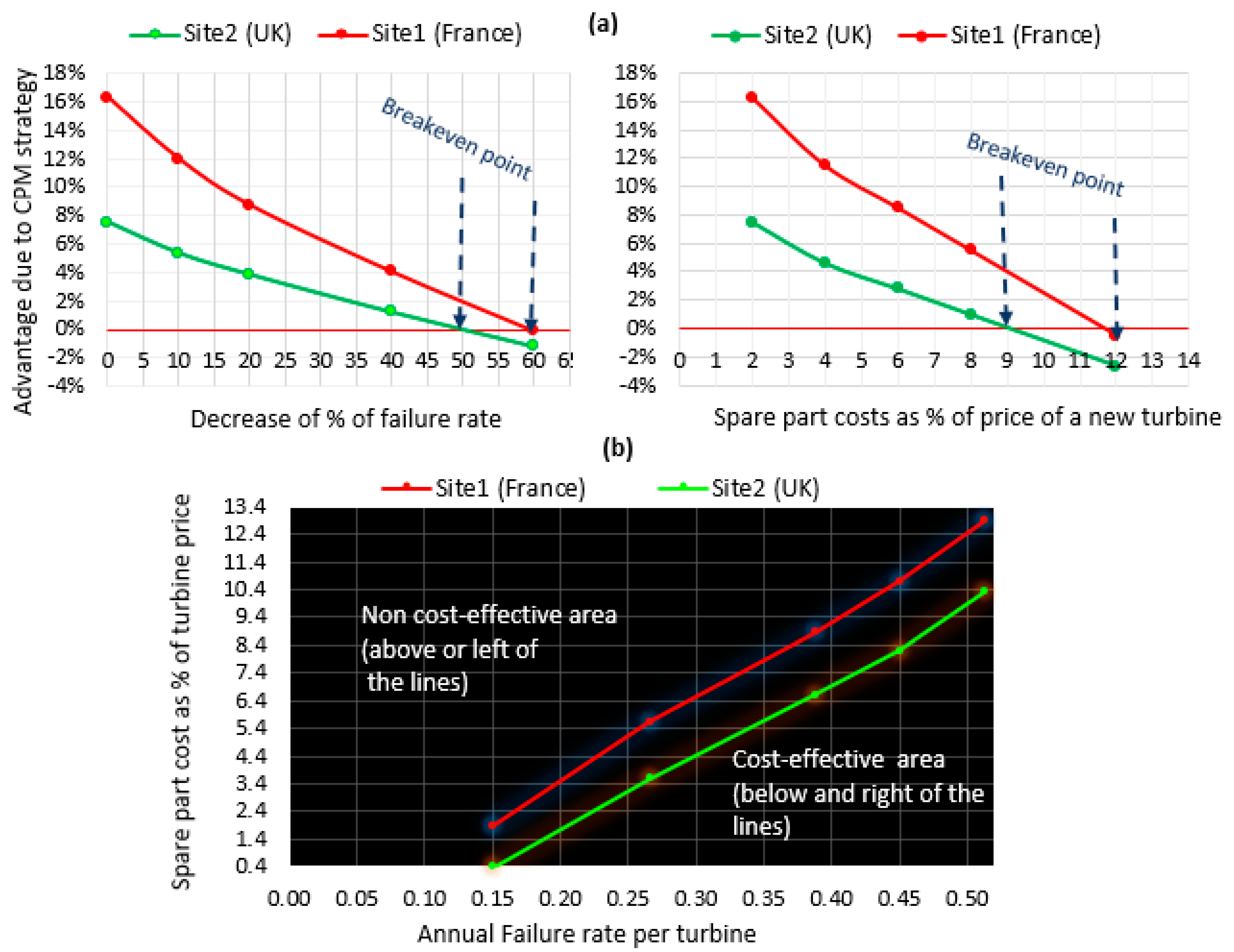
3.2. Sensitivity Analysis

Components’ failure rates greatly influence O&M costs. Only a few examples exist of operational tidal turbines, and so there is little experience of their behaviour; hence, assumptions are based on similar technologies from other industrial sectors [24]. It is argued that the tidal energy industry will follow a similar reliability growth curve as wind energy, and by increasing their operating hours, a tidal turbine will have a major annual failure rate of 0.065 [9]. If these failure rates are reduced, there may come a point when it may no longer be advantageous to use a planned maintenance strategy. Another input in the model is an assumed fixed spare parts cost over the farm’s life (25 years). There is a question of how a reduction in components’ annual failure rates or an increase in spare part costs will affect the advantage of the CPM strategy. A sensitivity analysis has tested this question, and the results are shown in Figure 10.

With respect to the number of failures, Figure 10a shows that the advantage of the CPM strategy is higher for the tidal farm in Site1 (France) compared to Site2 (UK). As mentioned earlier, a failure is typically more disruptive to power generation at Site1 than at Site2, and therefore the reduction of failure due to the CPM strategy has a more pronounced effect at Site1. As the failure rate reduces, there is less benefit from a planned maintenance strategy. The advantage will go to zero or become negative if the annual failure rate per turbine decreases by 50% or more (~0.26 failure/yr per turbine) in Site1 (France) and 60% or more (~0.15 failure/yr per turbine) in Site2 (UK). With respect to spare-part costs, Figure 10 shows that the advantage of the CPM strategy will go to zero or become negative if the spare-part cost is 10% or more (~€78,000 per turbine per year or 28 €/MWh) in Site1 (France) and 12% or more (~€97,000 per turbine per year or 17 €/MWh) in Site2 (UK). So, if failures are rare or if the spare-part costs for CPM are particularly expensive, then carrying out the CPM strategy may not be financially beneficial.

This sensitivity analysis leads to an interesting illustration of how these two factors, a cost factor and a risk factor, can combine to indicate when the CPM strategy is advantageous. In Figure 10b, there are five pairs of values for annual failure rates and spare part costs. At each of these five points on the plot, there is no benefit from choosing a CPM strategy compared with a CM strategy. The curve connecting these points acts as a border between the bottom right region on the plot where CPM strategy is advantageous and the top left region where CPM strategy is not advantageous. The graph can be used as a decision-making aid to understand the boundaries where a CPM strategy cannot be a cost-effective option under the known failure rates and spare part costs. This method may be extended to other pairs of constraints (e.g., distance from the port, grid rate, etc.).

This study has only considered two maintenance strategies (CM and CPM), and the sensitivity analysis was conducted only for two of the model parameters, namely failure rates and spare part costs. Further study is required to include other maintenance strategies, in particular a condition-based strategy that increases device reliability but incurs additional costs due to the deployment of monitoring systems such as vibration analysis, temperature monitoring, thermography and ultrasonic testing techniques [26].

The model developed in this study can be adapted to other emerging ORE technologies, such as floating offshore wind and wave energy converters.

4. Conclusions

A developed stochastic O&M model and scenarios have analysed the number of failures, downtime, energy income, and detailed O&M cost components of projected tidal stream farms in two locations in the northeast Atlantic: France and the UK. Two maintenance strategies are considered: a corrective (unplanned) maintenance (CM) strategy and a corrective combined with a preventive maintenance (CPM) strategy (at 5-year intervals) for a projected 20 MW tidal farm consisting of 10 horizontal axis stream turbines. The effect of planned maintenance on reducing the degradation of the tidal turbine is considered. A Weibull distribution using Monte-Carlo simulations has been used to model the device performance and a breakdown of the variable O&M activities and costs for the farms. The results are discussed with respect to the two maintenance strategies.

The projected tidal farm in the UK location (Site2) shows a considerably higher energy production (35%), due to the higher mean current velocity (on average by 22%), which increases the energy production and therefore the turbine capacity factor relative to the French site. Larger vessels, like DP vessels with cranes, are needed for a fixed tidal turbine. The DP vessel’s high accessibility and ability to operate at wave heights of up to 3 m and at wind speeds of 20 m/s lessen the effects of weather on the device’s downtime. The influence of weather on the two projects’ downtime at the sites in the UK and France was only 0.4% and 0.8%, respectively, which contributes to the high availability of the case studies. However, if vessels with restricted operational accessibility are used, the UK sites would have a shorter weather window waiting period, which could affect energy yields, O&M costs, and farm availability. For the Hs ≤ 2 m and wind speed of 20 m/s, for instance, the UK site would have a lower weather window waiting time of approximately 53% compared to the French location (Site1).

The study has discussed the uncertainties of the outcome, and sensitivity analyses are performed to understand the effect of the annual failure rates (a technical parameter) and the spare-part costs (an economic parameter) on the advantage of the CPM strategy.

This paper provides key insights into the trade-offs between corrective maintenance and combined corrective-preventive maintenance strategies, and boundaries where the CPM would not be financially advantageous are discussed. The method contributes to the decision-making process about which maintenance strategy would reduce the O&M cost without sacrificing the net energy income for the development of future tidal stream farms.

References

1. European Commission. Boosting Offshore Renewable Energy for a Climate Neutral Europe. 2020. Available online: https://ec.europa.eu/commission/presscorner/detail/en/IP_20_2096 (accessed on 8 December 2022).
2. Lewis, M.; Hara, R.O.; Fredriksson, S.; Maskell, J.; De Fockert, A.; Neill, S.P.; Robins, P.E. A standardised tidal-stream power curve, optimised for the global resource. Renew. Energy 2021, 170, 1308–1323. [Google Scholar] [CrossRef]
3. Yang, Z.; Ren, Z.; Li, Z.; Xu, Y.; Li, H.; Li, W.; Hu, X. A comprehensive analysis method for levelized cost of energy in tidal current power generation farms. Renew. Energy 2022, 182, 982–991. [Google Scholar] [CrossRef]
4. Collombet, R. Ocean Energy Key Trends and Statistics 2019; Ocean Energy Europe: Brussels, Belgium, 2020; pp. 10–13. [Google Scholar]
5. Sleiti, A.K. Tidal power technology review with potential applications in Gulf Stream. Renew. Sustain. Energy Rev. 2017, 69, 435–441. [Google Scholar] [CrossRef]
6. Hodges, J.; Henderson, J.; Ruedy, L.; Soede, M.; Weber, J.; Ruiz-Minguela, P.; Jeffrey, H.; Bannon, E.; Holland, M.; Maciver, R.; et al. An International Evaluation and Guidance Framework for Ocean Energy Technology 2O21 2-Task 12. IAn Int. Eval. Guid. Fram. Ocean Energy Technoglogy. IEA-OES. 2021. Available online: www.formasdopossivel.com (accessed on 20 April 2023).
7. Nachtane, M.; Tarfaoui, M.; Goda, I.; Rouway, M. A review on the technologies, design considerations and numerical models of tidal current turbines. Renew. Energy 2020, 157, 1274–1288. [Google Scholar] [CrossRef]
8. Segura, E.; Morales, R.; Somolinos, J.A.; López, A. Techno-economic challenges of tidal energy conversion systems: Current status and trends. Renew. Sustain. Energy Rev. 2017, 77, 536–550. [Google Scholar] [CrossRef]
9. Walker, S.; Thies, P.R. A review of component and system reliability in tidal turbine deployments. Renew. Sustain. Energy Rev. 2021, 151, 111495. [Google Scholar] [CrossRef]
10. Magagna, D.; Margheritini, L.; Alessi, A.; Bannon, E.; Boelman, E.; Bould, D.; Coy, V.; De Marchi, E.; Frigaard, P.; Guedes Soares, C.; et al. Workshop on Identification of Future Emerging Technologies in the Ocean Energy Sector; 27 March 2018, Ispra, Italy, EUR 29315 EN; JRC112635; European Commission: Luxembourg, 2018; ISBN 978-92-79-92587-0/978-92-79-92586-3. [CrossRef]
11. Word Economic Forum. A New Tidal Energy Project Just Hit a Major Milestone in Scotland. 2020. Available online: https://www.weforum.org/agenda/2020/01/tidal-renewable-energy-turbine-electricity-generation-scotland/ (accessed on 10 August 2022).
12. Lopez, A.; Moran, J.L.; Nunez, L.R.; Somolinos, J. Study of a cost model of tidal energy farms in early design phases with parametrization and numerical values. Application to a second-generation device. Renew. Sustain. 2020, 117, 109497. [Google Scholar] [CrossRef]
13. Neary, V.S.; Previsic, M.; Jepsen, R.A.; Lawson, M.J.; Yu, Y.; Copping, A.E.; Fontaine, A.A.; Hallett, K.C.; Murray, D.K. Methodology for Design and Economic Analysis of Marine Energy Conversion (MEC) Technologies; SANDIA REPORT; SAND2014-9040; Sandia National Laboratories: Livermore, CA, USA, 2014. [Google Scholar]
14. European Commission. LCEO Ocean Energy Technology Development Report 2018 EUR 29907 EN; European Commission: Brussels, Belgium, 2019.
15. European Union. An EU Strategy to Harness the Potential of Offshore Renewable Energy for a Climate Neutral Future; European Union: Luxembourg, 2020; p. 27. [Google Scholar]
16. Ioannou, A.; Angus, A.; Brennan, F. A lifecycle techno-economic model of offshore wind energy for different entry and exit instances. Appl. Energy 2018, 221, 406–424. [Google Scholar] [CrossRef]
17. Smart, G.; Noonan, M. Tidal Stream and Wave Energy Cost Reduction and Industrial Benefit: Summary Analysis. no. April. 2018, p. 21. Available online: https://www.marineenergywales.co.uk/wp-content/uploads/2018/05/ORE-Catapult-Tidal-Stream-and-Wave-Energy-Cost-Reduction-and-Ind-Benefit-FINAL-v03.02.pdf (accessed on 20 September 2022).
18. Rinaldi, G.; Portillo, J.C.C.; Khalid, F.; Henriques, J.C.C.; Thies, P.R.; Gato, L.M.C.; Johanning, L. Multivariate analysis of the reliability, availability, and maintainability characterizations of a Spar–Buoy wave energy converter farm. J. Ocean Eng. Mar. Energy 2018, 4, 199–215. [Google Scholar] [CrossRef]
19. BVG Associates. A Guide to an Offshore Wind Farm Updated and Extended. Publ. Behalf Crown Estate Offshore Renew. Energy Catapult, no. January. 2019, pp. 1–70. Available online: http://www.thecrownestate.co.uk/guide_to_offshore_windfarm.pdf (accessed on 25 April 2023).
20. Rinaldi, G.; Garcia-Teruel, A.; Jeffrey, H.; Thies, P.R.; Johanning, L. Incorporating stochastic operation and maintenance models into the techno-economic analysis of floating offshore wind farms. Appl. Energy 2021, 301, 117420. [Google Scholar] [CrossRef]
21. Lazakis, I.; Khan, S. An optimization framework for daily route planning and scheduling of maintenance vessel activities in offshore wind farms. Ocean Eng. 2021, 225, 108752. [Google Scholar] [CrossRef]
22. Neves-Moreira, F.; Veldman, J.; Teunter, R.H. Service operation vessels for offshore wind farm maintenance: Optimal stock levels. Renew. Sustain. Energy Rev. 2021, 146, 111158. [Google Scholar] [CrossRef]
23. Stålhane, M.; Vefsnmo, H.; Halvorsen-Weare, E.E.; Hvattum, L.M.; Nonås, L.M. Vessel Fleet Optimization for Maintenance Operations at Offshore Wind Farms under Uncertainty. Energy Procedia 2016, 94, 357–366. [Google Scholar] [CrossRef]
24. Lande-Sudall, D.; Stallard, T.; Stansby, P. Co-located deployment of offshore wind turbines with tidal stream turbine arrays for improved cost of electricity generation. Renew. Sustain. Energy Rev. 2019, 104, 492–503. [Google Scholar] [CrossRef]
25. Kolios, A.; Di Maio, L.F.; Wang, L.; Cui, L.; Sheng, Q. Reliability assessment of point-absorber wave energy converters. Ocean Eng. 2018, 163, 40–50. [Google Scholar] [CrossRef]
26. Ren, Z.; Shankar, A.; Li, Y.; Teuwen, J.J.E.; Jiang, Z. Offshore wind turbine operations and maintenance : A state-of-the-art review. Renew. Sustain. Energy Rev. 2021, 144, 110886. [Google Scholar] [CrossRef]
27. Karyotakis, A.; Bucknall, R. Planned intervention as a maintenance and repair strategy for offshore wind turbines. J. Mar. Eng. Technol. 2010, 9, 27–35. [Google Scholar] [CrossRef]
28. Vieira, M.; Henriques, E.; Snyder, B.; Reis, L. Insights on the impact of structural health monitoring systems on the operation and maintenance of offshore wind support structures. Struct. Saf. 2022, 94, 102154. [Google Scholar] [CrossRef]
29. Judge, F.; McAuliffe, F.D.; Sperstad, I.B.; Chester, R.; Flannery, B.; Lynch, K.; Murphy, J. A lifecycle financial analysis model for offshore wind farms. Renew. Sustain. Energy Rev. 2019, 103, 370–383. [Google Scholar] [CrossRef]
30. Lewis, M.; Neill, S.P.; Robins, P.; Hashemi, M.R.; Ward, S. Characteristics of the velocity profile at tidal-stream energy sites. Renew. Energy 2017, 114, 258–272. [Google Scholar] [CrossRef]
31. Coles, D.; Angeloudis, A.; Goss, Z.; Miles, J. Tidal stream vs. wind energy: The value of predictable, cyclic power generation in off-grid hybrid systems. Energies 2021, 14, 1106. [Google Scholar] [CrossRef]
32. Vennell, R.; Major, R.; Zyngfogel, R.; Beamsley, B.; Smeaton, M.; Scheel, M.; Unwin, H. Rapid initial assessment of the number of turbines required for large-scale power generation by tidal currents. Renew. Energy 2020, 162, 1890–1905. [Google Scholar] [CrossRef]
33. Deng, G.; Zhang, Z.; Li, Y.; Liu, H.; Xu, W.; Pan, Y. Prospective of development of large-scale tidal current turbine array: An example numerical investigation of Zhejiang, China. Appl. Energy 2020, 264, 114621. [Google Scholar] [CrossRef]
34. Faizan, M.; Badshah, S.; Badshah, M.; Haider, B.A. Performance and wake analysis of horizontal axis tidal current turbine using Improved Delayed Detached Eddy Simulation. Renew. Energy 2022, 184, 740–752. [Google Scholar] [CrossRef]
35. Nuernberg, M.; Tao, L. Experimental study of wake characteristics in tidal turbine arrays. Renew. Energy 2018, 127, 168–181. [Google Scholar] [CrossRef]
36. Ouro, P.; Ramírez, L.; Harrold, M. Analysis of array spacing on tidal stream turbine farm performance using Large-Eddy Simulation. J. Fluids Struct. 2019, 91, 102732. [Google Scholar] [CrossRef]
37. Segura, E.; Morales, R.; Somolinos, J.A. Cost assessment methodology and economic viability of tidal energy projects. Energies 2017, 10, 1806. [Google Scholar] [CrossRef]
38. Larsson, J. Transmission Systems for Grid Connection of Offshore Wind Farms HVAC vs HVDC Breaking Point; UPTEC ES 21010; Uppsala University: Uppsala, Sweden, 2021; ISSN 1650-8300. [Google Scholar]
39. Taketomi, N.; Yamamoto, K.; Chesneau, C.; Emura, T. Parametric Distributions for Survival and Reliability Analyses, a Review and Historical Sketch. Mathematics 2022, 10, 3907. [Google Scholar] [CrossRef]
40. Cain, N. Distinguishing between lognormal and Weibull distributions -time-to-failure data. IEEE Trans. Reliab. 2002, 51, 28–32. [Google Scholar] [CrossRef]
41. Bromideh, A. Discriminating Between Weibull and Log-Normal Distributions Based on Kullback-Leibler Divergence. Ekonom. ve İstatistik e-Dergisi 2012, 16, 44–54. [Google Scholar]
42. Wang, J.; Zhao, X.; Guo, X. Optimizing wind turbine’s maintenance policies under performance-based contract. Renew. Energy 2019, 135, 626–634. [Google Scholar] [CrossRef]
43. Abdollahzadeh, H.; Atashgar, K.; Abbasi, M. Multi-objective opportunistic maintenance optimization of a wind farm considering limited number of maintenance groups. Renew. Energy 2016, 88, 247–261. [Google Scholar] [CrossRef]
44. Herbert, G.M.J.; Iniyan, S.; Goic, R. Performance, reliability and failure analysis of wind farm in a developing Country. Renew. Energy 2010, 35, 2739–2751. [Google Scholar] [CrossRef]
45. Mudholkar, G.S.; Srivastava, D.K.; Kollia, G.D. A generalization of the Weibull distribution with application to the analysis of survival data. J. Am. Stat. Assoc. 1996, 91, 1575–1583. [Google Scholar] [CrossRef]
46. Thies, P.; Johanning, L.; Smith, G. Towards component reliability testing for marine energy converters. Ocean Eng. 2011, 38, 360–370. [Google Scholar] [CrossRef]
47. Nguyen, T.A.T.; Chou, S.Y. Improved maintenance optimization of offshore wind systems considering effects of government subsidies, lost production and discounted cost model. Energy 2019, 187, 115909. [Google Scholar] [CrossRef]
48. Papoulis, A.; Pillai, S.U. Probability, Random Variables, and Stochastic Processes, 4th ed.; McGraw-Hill: Boston, MA, USA, 2002; ISBN 0-07-366011-6. [Google Scholar]
49. De Andrés, A.; Macgillivray, A.; Guanche, R.; Jeffrey, H. Factors affecting LCOE of Ocean energy technologies: A study of technology and deployment attractiveness. In Proceedings of the 5th International Conference on Ocean Energy, Halifax, NS, Canada, 4–6 November 2014; pp. 1–11. Available online: https://inore-yaronguez.netdna-ssl.com/wp-content/uploads/2015/02/AdeAndres_AMacGillivray-2.pdf (accessed on 5 September 2022).
50. Gray, A.; Dickens, B.; Bruce, T.; Ashton, I.; Johanning, L. Reliability and O&M sensitivity analysis as a consequence of site specific characteristics for wave energy converters. Ocean Eng. 2017, 141, 493–511. [Google Scholar] [CrossRef]
51. OES-IEA. International Levelised Cost of Energy for Ocean Energy Technologies. 2015. Available online: https://www.ocean-energy-systems.org/oes-projects/levelised-cost-of-energy-assessment-for-wave-tidal-and-otec-at-an-international-level/ (accessed on 5 February 2023).
52. Meygen Ltd. Lessons Learnt from MeyGen Phase 1A Part 2/3: Construction Phase. no. May. 2018; p. 15. Available online: https://tethys.pnnl.gov/sites/default/files/publications/MeyGen-2017-Part1.pdf (accessed on 5 September 2022).
53. Frost, C. Cost Reduction Pathway of Tidal Stream Energy in the UK and France. TIGER Project 2019–2023. 2022. Available online: https://ore.catapult.org.uk/?orecatapultreports=cost-reduction-pathway-of-tidal-stream-energy-in-the-uk-and-france (accessed on 11 May 2023).
54. Stehly, T.; Duffy, P. 2020 Cost of Wind Energy Review. National Renewable Energy Laboratory. NREL/TP-5000-81209. Rep., no. December. 2021; p. 68. National Renewable Energy Laboratory. NREL/TP-5000-81209. Available online: https://www.nrel.gov/docs/fy22osti/81209.pdf (accessed on 11 May 2023).
Figure 1. Country-based tidal device types in 2020. Own elaboration using EMEC data source: http://www.emec.org.uk/marine-energy/tidal-developers/, accessed on 10 February 2023.
Jmse 11 01046 g001
Figure 2. Overview of the O&M model and the processing logic.
Jmse 11 01046 g002
Figure 3. Histograms of the current speed of both sites (top) and statistics of the current speed of the UK site (bottom) over 25 years. The mean current speed at the French site is lower than that at the UK site. Due to intellectual property concerns regarding industrial data, the statistics of French locations are not shown.
Jmse 11 01046 g003
Figure 4. Power calculation parameters used in the study (own elaboration based on industry consultations).
Jmse 11 01046 g004
Figure 5. The probability density function for various Weibull k (own elaboration).
Jmse 11 01046 g005
Figure 6. The average weather window waits in hours for 24 h of good weather at two locations. Hs is the significant wave height.
Jmse 11 01046 g006
Figure 7. Percentage breakdown of O&M as an example for the UK site.
Jmse 11 01046 g007
Figure 8. Histograms of CM and CPM strategies.
Jmse 11 01046 g008
Figure 9. Histograms of net energy income for CM and CPM strategies.
Jmse 11 01046 g009
Figure 10. (a) Left, sensitivity of failure rates; right, sensitivity of spare-part costs; and (b) combined effect of failure rate and spare-part cost on the advantage of CPM strategy.
Jmse 11 01046 g010