Abstract
This paper focuses on the finite-time formation-control problem of a multi-AUV formation under unknown perturbations with prescribed performance. First, the nonlinear AUV model is transformed into a second-order integral model using feedback linearization. Suitable prescribed performance functions are selected to constrain the control errors of AUVs within a preset range and convert AUV tracking errors into unconstrained tracking errors using an error-conversion function to facilitate controller design. Finite-time sliding-mode disturbance observers are designed for unknown disturbances in the ocean so that they can accurately estimate the unknown disturbances in finite time. Based on the unconstrained tracking error and the unknown disturbance observer, the fast terminal sliding-mode formation controller is designed so that the multi-AUV formation can converge in finite time. Finally, the simulation experimental results show that the finite-time formation-control method with prescribed performance proposed in this paper can better cancel the unknown disturbance in the ocean in finite time and improve the robustness of the multi-AUV formation control.
1. Introduction
At present, countries all over the world are actively carrying out the exploration, development, and utilization of marine resources. Autonomous underwater vehicles (AUVs), as a new type of marine-exploration equipment with strong autonomy, low cost, good versatility, rapid response, and good mobility, have been widely used in marine-resource exploration, underwater engineering, and other aspects [1,2]. However, due to the constraints of energy, AUVs are beginning to be overwhelmed when facing some demanding tasks. As a result, multi-AUV collaboration, information sharing, and joint task completion have become the new direction of AUV development [3,4]. For example, in marine-environment monitoring, if only a single AUV is used to complete marine-environment-monitoring work, the efficiency will be low; if multiple AUVs are used to complete marine-environment-monitoring work, the efficiency will be greatly improved.
Multi-AUV formation-control methods can be divided into centralized control and distributed control. Consensus control is a distributed control, where each AUV obtains information about the state of its neighboring AUVs through sensors to achieve control. The consensus problem for multi-agent systems (MASs) with semi-Markovian jump parameters under the influence of disturbances has been studied [5]. The consensus of MASs with semi-Markovian jump parameters and external disturbances is solved by a non-fragile controller with randomly occurring gain fluctuations using an extended dissipative approach. In the centralized-control method, a single leader connecting all AUVs has global team information and manages the information to ensure that the mission is accomplished. For the centralized-control method, a powerful leader can greatly improve the overall performance of a multi-AUV formation. The disadvantage of this scheme is that the whole system is highly dependent on the leader and the unknown disturbances of the ocean, etc., make the system less robust. The leader–follower control strategy belongs to one of the centralized-control methods. The leader–follower method transforms the control problem of a multi-AUV formation into a problem of whether the distance error and angle error between the leader and the follower converge [6].
Park [7] investigated an adaptive master–slave formation control of underdriven AUVs. Wang [8] used the leader–follower method and a filtered backstepping technique to solve the formation-control problem of multiple AUVs. Then, an adaptive sliding-model-based master–slave strategy was proposed in the literature [9] to solve the formation-control problem influenced by disturbances and uncertain dynamics. In [10], Desai constrained the distance and attitude angle between the leader and the follower so that the leader and the follower could maintain a stable formation and designed a formation controller based on the spacing and the attitude angle. In [11], Fahimi designed a backstepping sliding-mode formation controller based on the leader–follower strategy for the nonlinear AUV model, combining the advantages of backstepping control and sliding-mode control, which can solve the jitter problem that occurs in a small range.
For the problems of unknown disturbances and an AUV’s own unmeasurable velocity information in a complex ocean environment, external disturbances were counteracted in [12] by adjusting the control gain of the formation-coordination controller, and an ESO observer was designed to calculate the voyager’s own velocity information. In [13], a fixed-time perturbation observer and a velocity observer were designed so that an AUV could quickly estimate the perturbation and velocity quantities to accomplish the trajectory-tracking task. In [14], adaptive RBF was used to converge the unknown perturbations and model uncertainties and a velocity-state observer was designed based on a bio-inspired model so that an AUV could estimate its velocity without relying on the model.
Another problem in formation control is the slow convergence of formation error due to the random distribution of AUVs in the initial stage of formation, so finite-time formation control has become a hot research topic in recent years. Gao [15] proposed a fixed-time-based multi-AUV leader–follower formation-control method. To achieve the finite-time convergence of formation-tracking error, Xia [16] designed a two-loop controller to control a multi-AUV formation and developed a controller based on a neural network and a conditional integrator to deal with model uncertainty and disturbances. In addition, the authors of [17] designed an AUV formation-control algorithm using the command-filter backstepping method and fixed-time theory, which successfully improved the system’s convergence speed.
Prescribed performance control was first proposed by the Greek scholars Bechlioulis and Rovithakis [18,19] in 2008 as a control method to change the error-convergence rate to improve a system’s performance. The principle of prescribed performance control is to design a performance function to constrain the system error and to design an error-conversion function to convert the constrained error into unconstrained error to facilitate controller design. This method can improve the transient performance of a system by reducing the system overshoot and steady-state error and has therefore received wide attention.
Prescribed performance control was initially mainly applied in the field of generalized nonlinear systems and combined with methods such as sliding-mode control, backstepping control, and adaptive RBF to solve problems such as the model uncertainty of nonlinear systems [20,21]. For example, a new performance function and error-transformation function were designed (Refs. [22,23], respectively), and the initial value of the boundary of the performance-function constraint was set to infinity, which ensured that the initial value of the system error could not be determined but that the performance function could still be used to constrain the error when the initial value of the system error could not be determined. In order to reduce the computational effort of algorithms such as neural-network approximation and solve specific problems, a new control method based on prescribed performance control was proposed in [24], which discarded algorithms such as neural-network approximation. Since then, many scholars have proposed many “no-approximation,” “no-estimation,” and “no-model” control schemes based on prescribed performance [25,26,27], which greatly reduce the need for accurate models and are therefore useful in the study of uncertain nonlinear systems. Uncertain nonlinear systems have been widely used in the study of uncertain nonlinear systems [28,29]. To address the problem of unpredictable system-output states, the authors of [30] used passive methods to solve the problem of prescribed-performance-output feedback. The authors of [31], on the other hand, used input-driven filters to obtain unmeasurable higher-order states for output-feedback control. In addition, prescribed-performance control has started to be used in a large number of practical applications, such as dead zones [32,33], faults [34,35], saturation [33], and the study of switching systems [36].
In recent years, prescribed-performance control has been widely used in robotic systems [28], space-vehicle systems [29], and multi-intelligent-body systems [37]. In [38], adaptive-terminal sliding-mode controllers based on prescribed performance have been proposed.
Most of the current research results focus on analyzing the stability and steady-state behavior of the closed-loop system without fully considering transient performance such as formation time in AUV formation control. Based on the above research results, this paper proposes a finite-time formation-control method for multi-AUV formation with unknown perturbations with pre-defined performance, taking into account the steady-state performance and transient performance of the formation and considering the influence of unknown perturbations on the formation control. The specific contributions of this paper are summarized as follows:
- An improved prescribed-performance function is proposed to constrain the constrained state-tracking error so that the system-tracking error is constrained to a preset range, and an error-conversion function is used to convert the system-tracking error to an unconstrained tracking error to facilitate controller design.
- For unknown disturbances in the ocean, finite-time sliding-mode disturbance observers are designed so that they can accurately estimate unknown disturbances in finite time.
- The feedback-linearization method is applied to transform the nonlinear AUV model into a second-order integral model and design a fast terminal sliding-mode formation controller based on unconstrained tracking errors and unknown perturbation observations so that the multi-AUV formation can converge in a limited amount of time.
2. Building Nonlinear AUV Model and Feedback Linearization
2.1. Nonlinear AUV Model
To study the motion of the AUV, the fixed-coordinate system {E} and the motion-coordinate system {O} were established and are shown in Figure 1.
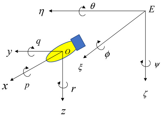
Figure 1.
Coordinate-system diagram.
A fixed point at sea level is usually chosen as the origin of the fixed-coordinate system, where the axis points are due north and the axis points are due east. In order to simplify the nonlinear AUV model, the center of gravity of the AUV is chosen as the origin of the motion-coordinate system {O}, where the axis is located in the longitudinal mid-profile and points to the bow of the AUV and the axis is perpendicular to the longitudinal mid-profile and points to the starboard side of the AUV.
In model building, it can be assumed that the AUV studied in this paper is a rigid body with a certain mass distribution, and the effect of its transverse rocking motion is not considered when the AUV is operating underwater; i.e., the transverse rocking-attitude angle and angular velocity are kept at the desired values. In the following section, the nonlinear AUV model and the feedback linearization process are based on this assumption.
For the purpose of the following study, the following motion variables are defined:
Define the position vector in a fixed-coordinate system:
Define the posture vector in a fixed-coordinate system:
Using Equations (1) and (2), the position and posture vector in a fixed-coordinate system are modeled as:
Define the linear velocity in the motion-coordinate system:
Define the angular velocity in the motion-coordinate system:
Using Equations (3) and (4), the velocity vector in the motion-coordinate system is modeled as:
Define the force in the motion-coordinate system:
Define the moment in the motion-coordinate system:
Using Equations (5) and (6), the force and moment in the motion-coordinate system are modeled as:
denotes the three-dimensional Euclidean space, and denotes the three-dimensional torus; i.e., there are three angles in the range .
The kinematic and kinetic mathematical model-derivation process and the model parameters of the AUV are shown in [11]. Combining the AUV kinematic model and the dynamics model, the nonlinear mathematical AUV model’s vector expression can be obtained as:
2.2. AUV Feedback-Linearization Model
As can be seen in Equation (10), the nonlinear AUV model is still very complicated, even if it is written in vector form. In this subsection, we simplify the nonlinear AUV model using the transformation method to make the complex problem simple. Using coordinate transformation, we can transform the nonlinear AUV model in the motion-coordinate system to a specific coordinate system in which the nonlinear model will realize the decoupling of each control channel and transform into a second-order integral model.
According to [39], the AUV model is transformed appropriately:
where is the sum of the inertia matrix and the additional inertia matrix. denotes the control-input forces and moments. By synthesizing the three terms of the model (, , and ) into a column vector (), Equation (11) can be transformed into:
In Equation (12), a mathematical model with three axial thrusters and two rudders is considered, replacing the controller input T in Equation (12) with the thrust of the axial thrusters , , and and the rudder angles and . The vector will be formed by and .
Define the function:
Define the function:
Using Equations (13) and (14), Equation (12) is transformed into the following vector form:
Among them, , , and .
Vector field: The nonlinear first-order model is taken as the following equation:
where , , and are smooth enough over the definition-domain , and the mapping and are vector fields over the domain of definition D.
Lie derivative: derivative of in Equation (16).
where and are said to be the Lie derivative of along the smooth-vector field .
Define the output function:
Using Equation (18), the dynamics of the AUV are modeled as:
The basic idea of feedback linearization is to find an appropriate coordinate transformation and control rate after the coordinate transformation.
The coordinate transformation is:
By transforming the coordinates, we obtain:
The transformation yields:
In a given coordinate system, the control input can be expressed as:
Then, the second-order integral AUV model in the new coordinate system after transformation can be obtained under the action of Equations (19) and (23).
The linearized mathematical AUV model can be obtained as:
where is the position information of the AUV after the coordinate transformation, is the speed information of the AUV after the coordinate transformation, and is the control input of the AUV after the coordinate transformation.
3. Problem Description and Preparatory Knowledge
3.1. Problem Description
The linearized mathematical model for an AUV subjected to unknown disturbances in the ocean should be:
where is the bounded unknown environmental perturbation.
Robustness is divided into stable robustness and performance robustness, so to achieve robust control of an AUV formation, it is necessary to ensure the steady-state performance of the formation system as well as to make it have good transient performance. However, most of the control methods and strategies only consider the steady-state performance of an AUV formation by setting the initial state and selecting the appropriate control gain to make the tracking error converge near zero, without considering the transient performance such as the convergence speed and overshoot. It has been found that introducing a prescribed-performance function to limit the error range can control the overshoot of the system within the desired range, whereas using a finite-time controller can reduce the convergence time of the system. Therefore, it is the goal of this paper to improve the transient performance of the system while ensuring the steady-state performance by accurately estimating the unknown external disturbances in finite time.
3.2. Preparatory Knowledge
The prescribed performance is to specify a region defined by the progressive-decay function according to the prescribed-performance function so that the tracking error is always within the preset region and the transient error of the system is guaranteed.
Definition 1.
If a function of a class satisfies the following conditions, then it is referred to as a performance function.
Condition 1: is continuously derivable and monotonically decreasing, and
Condition 2:
The commonly used performance functions are the hyperbolic tangent and exponential forms, with the exponential form as follows:
where , , and are positive constants; and are the initial and steady-state values of the performance function, respectively; and is the decay rate of the performance function.
The system tracking error is defined, and the performance function is used to constrain the error bounds so that they satisfy the following form:
where . A schematic diagram is shown in Figure 2.
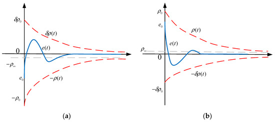
Figure 2.
Diagram of performance-constrained error-response curves, where (a) is the error-response curve when and (b) is the error-response curve when .
In Equation (30) and Figure 2, it can be seen that the constraint on the tracking error of the system can be achieved when the initial error of the system satisfies . At this time, the maximum overshoot of the system is less than , the minimum convergence rate of the tracking error depends on the decay rate of the performance function , and the maximum value of the steady-state error depends on the size of . Therefore, the desired error-response curve can be obtained by reasonably setting the parameters in the performance function and the value of .
When using the performance function to constrain the system tracking error, it increases the complexity of the controller design. Therefore, a conversion needs to be introduced to convert the constrained tracking error to an unconstrained tracking error by constructing the error-conversion equation as:
According to Equation (30), the error-conversion function satisfies the following properties:
Property 1: is strictly monotone and smooth over the domain of definition.
Property 2: when and .
Property 3: when and .
The selection of satisfying the conditions based on the above properties is as follows:
From Property 1, we know that is strictly monotonically increasing, so the inverse transformation of can be obtained as follows:
If can be bounded for any , the constraint relation in Equation (30) holds. In summary, the control problem with a bounded tracking error is converted into a stable control problem, described by Equation (33), via the error-conversion formula, and the design idea is shown in Figure 3.
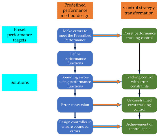
Figure 3.
Prescribed performance-design ideas.
Lemma 1.
Ref. [40]: For the nonlinear system
If there exists a continuous and positive definite function whose derivative satisfies:
where , , , and , then System (18) is stable in finite time and the convergence time () satisfies the following relation:
where satisfies .
4. Performance-Function Design and Error Transformation
The AUV feedback-linearization model is shown below:
The trajectory-tracking error is according to Equation (30), and in Figure 2, it is shown that the convergence process of the system error will also be fixed when the decay rate of the performance function () is determined. If the convergence rate is too fast, it leads to a large controller-output torque value in the initial stage. To solve this problem, the performance function given in this paper is improved to ensure the stable convergence of the tracking error on the premise that the convergence rate can be dynamically selected.
4.1. Performance-Function Improvement
In Equation (30), the trajectory-tracking error should satisfy the following constraint:
The constraint on the systematic-tracking error is achieved when the initial error of trajectory tracking () satisfies . When the exponential performance function is chosen to constrain the error, the convergence rate of the tracking error depends on the exponential term , but the relationship between them is not intuitive. Therefore, the original performance function in Equation (29) is improved.
Proposition 1.
Design a newly performance function containing convergence time with the following expression:
where , , , and are the parameters to be adjusted; is the decay rate; and is the settable time when the performance function reaches .
Proof of Proposition 1.
The next step is to demonstrate that the newly designed performance function satisfies the requirements of Definition 1 in Section 3.
Step 1: Calculate the parameters to be rectified according to the constraints , , , and .
From Equation (29), the new performance function satisfies the same initial and terminal conditions, i.e., and , respectively, and the new performance function must have consecutive first-order derivatives and second-order derivatives, as follows:
Let , according to the above conditions, and can be obtained as follows:
Step 2: Prove that the new performance function is monotonically decreasing and .
It follows from the above that and . If holds for any , then it can be shown that the new performance function is monotonically decreasing and that .
When , the derivative of the new performance function () is obtained from the values of , , , , and as follows:
From Equation (42) we obtain , so the above problem requires proving that when , , where is as follows:
Let and . Since , the above equation can be transformed as follows:
The boundary values of are and .
The derivative of with respect to is given as follows:
The boundary values of are and . The derivative of yields the second-order derivative of as follows:
According to Equation (46), we can obtain , so is monotonically decreasing. Since and , we obtain , so is monotonically increasing. Similarly, because and , . Combined with the above analysis, for any , holds (when and only when and ); that is, the new performance function () is constant and decreasing, satisfying the requirements of Definition 1 in Section 3.
In summary, it can be seen that the new potential-energy function satisfies the definition of the performance function when the parameters in Equation (39) are taken as shown in Equation (41). Meanwhile, according to the proof process in Step 2, an implicit conclusion can be obtained where the terminal time and the decay rate have no mutual-constraint relationship and can be taken arbitrarily. Therefore, compared with the traditional exponential-performance function, the new type of performance function has the following advantages:
Advantage 1: You can set the terminal convergence time by yourself according to the actual demand.
Advantage 2: When the terminal convergence time is determined, a suitable decay rate can be selected to avoid excessive controller-output torque in the initial stage.
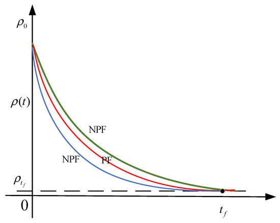
The effect of the traditional exponential-performance function compared to the new convergence-time performance function is shown in Figure 4. As can be seen in Figure 4, when both performance functions reach steady state at the same time, the new convergence-time performance function can change the convergence rate by adjusting the value of the decay rate , which can protect the controller and the actuators. □
Figure 4.
Performance-function comparison diagram.
4.2. Error Conversion
The error-conversion function takes the form of Equation (32) as follows:
The trajectory-tracking error for the ith follower in the formation is , so the following equation is available:
An inverse transformation of Equation (47) yields the following:
where .
The derivative of the conversion error is given as follows:
where . The second-order derivative of is obtained by deriving Equation (50) as follows:
5. Prescribed Performance-Based Formation-Controller Design under Unknown Perturbations
The novel convergence-time performance function is designed to constrain the trajectory-tracking error. To facilitate the design of the controller, the error-conversion function is used to convert the tracking error with constraints to the unconstrained error, and the converted error is used as the input to the controller. Meanwhile, it is known from System (26) that when the unknown disturbance to the AUV is observable, the formation controller based on the disturbance observer needs to be designed to ensure the stability of the system-state quantity by changing the controller output , and the specific control-block diagram is shown in Figure 5.
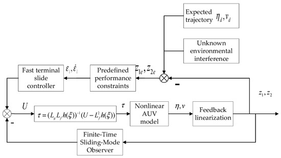
Figure 5.
Diagram of the AUV control system.
5.1. Sliding-Mode Interference-Observer Design
5.1.1. Common Slip-Mode Interference Observer
A sliding-mode disturbance observer is designed for System (26) as follows:
where is the error slip surface, is the estimate of the system , is the estimate of the unknown disturbance, is the parameter to be designed, and . The derivation of leads to the following equation:
In Equation (53) above, it can be seen that the state-error sliding-mode surface converges asymptotically to zero when , whereas the unknown perturbation-estimation error tends to be near the zero value.
5.1.2. Finite-Time Sliding-Mode Interference Observer
The ordinary sliding-mode perturbation observer can only guarantee the asymptotic convergence of the perturbation-observation error and cannot achieve fast convergence in finite time. Therefore, to improve the convergence speed, the ordinary sliding-mode perturbation observer is improved by adding a power term with the following equation:
where , , and are the parameters to be designed; and are positive odd numbers; and .
For a system (System (26)) that receives unknown external perturbations, the external perturbations can be observed using a sliding-mode perturbation observer (Equation (54)), and the perturbation-estimation error can be made to converge to zero in finite time by means of rectifying the parameters.
The following Lyapunov function is chosen:
The derivation of the function leads to the following equation:
If the parameters in Equation (56) satisfy , , and , it can be deduced that:
In Equation (57), , so according to Lemma 1, the state-error sliding-mode surface can converge to zero in finite time , and the unknown perturbation-estimation error also converges to zero in finite time .
5.2. Sliding-Mode Interference-Observer Design
The fast terminal slide surface is defined as shown below:
where is the converted error, and are the parameters to be designed, and . and are positive odd numbers, and .
The derivation of Equation (58) leads to the following equation:
where .
In order to ensure the control effect while eliminating jitter, the convergence law containing two inverse functions is designed in this paper, and the expressions are shown below:
In the above equation, it can be seen that plays a dominant role in speeding up the system error to reach the slipform surface when it is far away from the slipform surface and that plays a dominant role in reducing the effect of jitter while ensuring the convergence speed when the system error is approaching the slipform surface. The combination of these two parts can ensure the quality of motion of the system state during the approach to the slipform surface.
The formation-control law can be obtained according to Equations (54), (59), and (60) as follows:
where , , and are the parameters of the positive design.
5.3. Formation-Controller Stability Analysis
When the AUV formation receives the effect of an external bounded unknown perturbation, the AUV-formation trajectory-tracking error and velocity error can be made to converge to a value near zero in finite time by adjusting the parameters under the action of the perturbation observer in Equation (38) and formation control law in Equation (45).
The Lyapunov function is chosen as follows:
where .
The derivation of leads to the following equation:
By substituting the formation-control law (Equation (62)) into Equation (63) it can be deduced that:
where .
Let , , , , , and . Therefore, it can be deduced that:
When , it follows from Lemma 1 in Section 3 that the error system can converge to near zero in finite time and that the convergence time satisfies the following equation:
Equation (58) is zero when the error system arrives at the slipform surface from any initial state, and it can be deduced that:
It is stated in [41] that the convergence time of the error on the slipform surface from a non-zero value to a zero value is:
In summary, the error system can converge to a value near zero in finite time when under the action of the perturbation observer in Equation (38) and the formation control law in Equation (45).
6. Simulation Verification and Analysis
6.1. Perturbation-Observer Simulation Validation
To verify the effectiveness and superiority of the finite-time sliding-mode observer designed in this paper, simulations were performed to compare with the ESO observer designed in [42] and the ordinary sliding-mode observer in Equation (36). The ESO observer was designed as follows:
The parameters were designed as , , , , and . The unknown perturbations were designed as follows:
where .
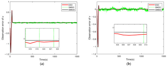
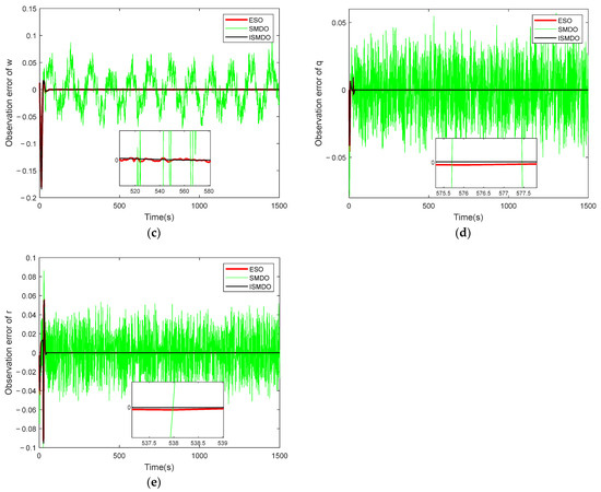
Figure 6.
Velocity-state observation-error diagram, where (a) is the error diagram of the longitudinal-velocity observation, (b) is the error diagram of the transverse-velocity observation, (c) is the error diagram of the vertical-velocity observation, (d) is the error diagram of the longitudinal-angular-velocity observation, and (e) is the error diagram of the bow-angular-velocity observation.
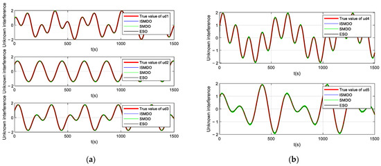
Figure 7.
Comparison graphs of unknown disturbance observations, where (a) is an observation-comparison graph of , , and , and (b) is an observation-comparison graph of and .
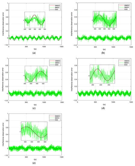
Figure 8.
Error plots of unknown perturbation observations, where (a) is the observation-error plot of , (b) is the observation-error plot of , (c) is the observation-error plot of , (d) is the observation-error plot of , and (e) is the observation-error plot of .
Figure 6 shows a plot of the velocity-state observation error. It can be seen in the figure that the observation error of the ordinary sliding-mode observer had significant fluctuations due to the presence of the sign function, whereas the observation errors of the ESO observer and the ISMDO observer both converged quickly to a value near zero, indicating the effectiveness of the design parameters. Figure 7 and Figure 8 show the observation plots of the unknown disturbance and the observation error. Since the disturbance was a high-frequency vibration signal, there was some fluctuation in the observation error. In Figure 8, it can be seen that the ESO and ISMDO observations were close to each other and that the perturbation-observation error fluctuated in the range of [−0.05, 0.06], but the ISMDO error was smaller and its observation results were more accurate.
6.2. Simulation Verification of Prescribed Performance Controllers
To verify the superiority of the prescribed-performance-based fast terminal sliding-mode controller (PP-IFTSMC) designed in this paper, a single AUV-comparison experiment was designed to compare it with adaptive fast terminal sliding-mode (AFTSMC), normal fast terminal sliding-mode (FTSMC), and non-singular terminal sliding-mode controllers (NTSMC) for simulation.
To reduce the jitter of the controller, the hyperbolic tangent function was used to replace the symbolic functions in PP-IFTSMC and NTSMC. The PP-IFTSMC controller from this paper was designed as follows:
The controller parameters were , , , , , , , , and . The performance-function parameters were , , , , and .
The adaptive fast terminal sliding-mode controller (AFTSMC) was designed as follows:
The controller parameters were , , , , and .
The fast terminal slip-mold controller (FTSMC) was designed as follows:
The controller parameters were , , , , , , , and .
The non-singular terminal sliding-mode controller (NTSMC) was designed as follows:
The slide surface was designed as . The controller parameters were , , , , , and .
The designed AUV’s desired trajectory was:
The initial states of the AUV were , , and . The bow angle was in the initial range of [0, 1] rad, and the other states were initialized to 0. The current velocity in the simulation environment was 0.2 m/s and the flow direction was 30°. The simulation-comparison results are shown in Figure 9 and Figure 10.
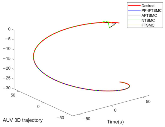
Figure 9.
The 3D trajectory-tracking effect of the AUV using different controllers.
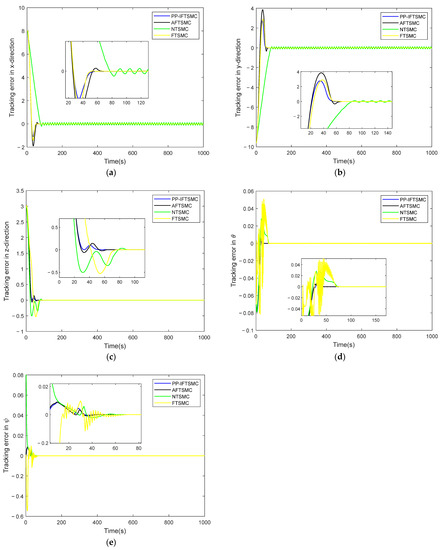
Figure 10.
Diagrams of AUV position and attitude-tracking errors using different controllers, where (a) is the northward trajectory-tracking error, (b) is the eastward trajectory-tracking error, (c) is the vertical trajectory-tracking error, (d) is the longitudinal-inclination-angle-tracking error, and (e) is the bow-angle-tracking error.
In Figure 9, the 3D trajectory-tracking results of the AUV using different controllers are shown, and it can be seen that all four controllers could make the AUV track the desired trajectory better. In Figure 9, it can be seen that the controller designed in this paper (PP-IFTSMC) could track the desired trajectory faster. Figure 10 shows the plot of the AUV attitude-tracking error. From Figure 10, it can be seen that the controller of this paper had the fastest convergence speed of attitude-tracking error, and the error curve in the initial state was very smooth and had less fluctuation. The other controllers had obvious error fluctuation and jitter phenomena. This shows the effectiveness of the performance-constraint function designed in this paper.
6.3. Simulation Verification of the Prescribed Performance-Formation Controller
Simulation experiments were designed to verify the effectiveness of path tracking based on the prescribed-performance AUV formation controller (Equation (61)). A current disturbance with a maximum flow velocity of 0.5 m/s and a flow direction of was considered. The unknown perturbation was designed as follows:
The designed AUV’s desired trajectory was:
The initial states of the follower AUV were m, m, and m. The initial values of longitudinal inclination angle rad, bow angle rad, m/s, and all other velocity and angular-velocity quantities were initialized to 0. The simulation added a current disturbance with a current velocity of 0.5 m/s and a current direction of 30°. The parameters m and were used in the formation constraints. The controller parameters were , , , , , , , , and . The performance-function parameters were , , , , and .
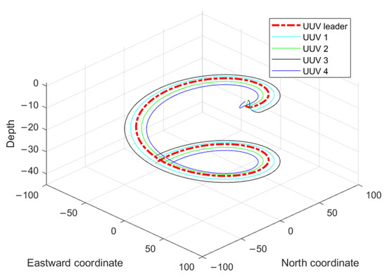
Figure 11.
3D trajectory diagram of the AUV formation under an unknown disturbance.
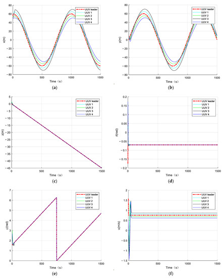
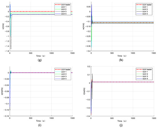
Figure 12.
AUV formation position, attitude, and velocity tracking-effect diagrams, where (a) is the AUV’s northward trajectory, (b) is the AUV’s eastward trajectory, (c) is the AUV’s vertical trajectory, (d) is the AUV’s longitudinal-inclination-angle state, (e) is the AUV’s bow-angle state, (f) is the AUV’s longitudinal velocity, (g) is the AUV’s lateral velocity, (h) is the AUV’s vertical velocity, (i) is the AUV’s longitudinal-inclination-angle velocity, and (j) is the AUV’s bow-angle velocity.
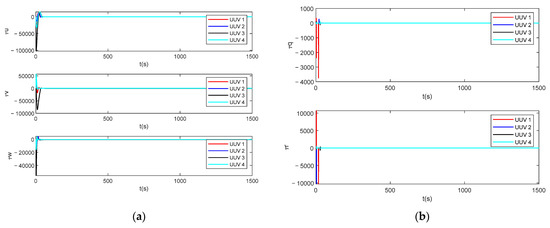
Figure 13.
Follower AUV’s control input, where (a) is an observation-comparison graph of , , and , and (b) is an observation-comparison graph of and .
In Figure 11, it can be seen that the multiple AUVs could maintain their formation to complete the trajectory tracking when there was an unknown bounded disturbance in the outside world, under the action of the disturbance observer (Equation (54)) and the formation controller (Equation (61)). In Figure 12, it can be seen that the velocity of the follower AUV fluctuated slightly under the influence of the perturbation but tended to be near the desired value. Figure 13 shows the control input of the follower AUV, and it can be seen that the control input of the follower AUV tended to be stable and converged around the zero value in a short time. Figure 14 and Figure 15 show the unknown disturbance observation results and the observation error graphs, respectively. From Figure 14 and Figure 15, we can see that the disturbance observer observation results are more accurate, but there are some fluctuations in the observation error because the disturbance is a high-frequency vibration signal.
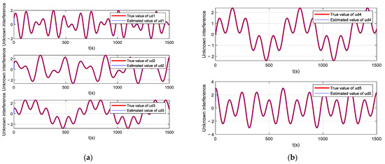
Figure 14.
Follower AUV’s control input, where (a) is a linear-velocity-control input and (b) is an angular-velocity-control input.
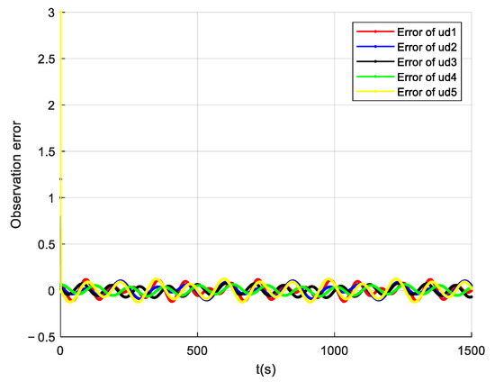
Figure 15.
Unknown perturbation-observation error.
7. Conclusions
This paper focused on the finite-time formation-control problem of a multi-AUV formation under unknown perturbations with prescribed performance. First, a five-degrees-of-freedom nonlinear model of an AUV was established, and it was processed using feedback linearization to obtain a second-order integral model of the AUV. When performing AUV formation control, the design of the formation-control strategy was carried out based on the pilot-following method. In order to resist external disturbances and ensure the steady-state performance of the formation, a finite-time sliding-mode disturbance observer was designed to achieve accurate estimations of unknown disturbances in finite time. A suitable prescribed-performance function was selected to constrain the control error of the AUV within a preset range, and an error-conversion function was used to convert the AUV tracking error to an unconstrained tracking error. Based on the unconstrained tracking error and the unknown disturbance observations, the fast terminal sliding-mode formation controller was designed so that the multi-AUV formation could converge in a limited time. Finally, the stability and effectiveness of the controller designed in this paper was verified by simulation experiments. In the future, the problem of formation control based on complex dynamic models and the problem of describing the control of communication delay by stochastic processes are to be further investigated.
Author Contributions
Conceptualization, J.L. and Z.T.; methodology, J.L.; software, J.L.; validation, J.L. and Z.T.; formal analysis, J.L.; investigation, J.L. and Z.T.; resources, J.L.; data curation, H.Z.; writing—original draft preparation, J.L.; writing—review and editing, W.L. and Z.T.; visualization, H.Z. and Z.T.; supervision, J.L.; project administration, J.L.; funding acquisition, J.L. All authors have read and agreed to the published version of the manuscript.
Funding
This research was funded by the National Natural Science Foundation of China (grant No. 5217110503), the research fund from Science and Technology on Underwater Vehicle Technology (grant No. JCKYS2021SXJQR-09), and the Natural Science Foundation of Shandong Province (grant No. ZR202103070036).
Institutional Review Board Statement
Not applicable.
Informed Consent Statement
Not applicable.
Data Availability Statement
Not applicable.
Conflicts of Interest
The authors declare no conflict of interest.
References
- Sun, Y.; Ling, J.; Chen, X.; Kong, F.; Hu, Q.; Biancardo, S.A. Exploring Maritime Search and Rescue Resource Allocation via an Enhanced Particle Swarm Optimization Method. J. Mar. Sci. Eng. 2022, 10, 906. [Google Scholar] [CrossRef]
- Liu, Y.; Wang, M.; Su, Z.; Luo, J.; Xie, S.; Peng, Y.; Pu, H.; Xie, J.; Zhou, R. Multi-AUVs Cooperative Target Search Based on Autonomous Cooperative Search Learning Algorithm. J. Mar. Sci. Eng. 2020, 8, 843. [Google Scholar] [CrossRef]
- Zhao, Z.; Hu, Q.; Feng, H.; Feng, X.; Su, W. A Cooperative Hunting Method for Multi-AUV Swarm in Underwater Weak Information Environment with Obstacles. J. Mar. Sci. Eng. 2022, 10, 1266. [Google Scholar] [CrossRef]
- Rego, F.; Hung, N.T.; Pascoal, A.M. Cooperative path-following of autonomous marine vehicles: Theory and experiments. In Proceedings of the 2018 IEEE/OES Autonomous Underwater Vehicle Workshop (AUV), Porto, Portugal, 6–9 November 2018. [Google Scholar]
- Sakthivel, R.; Parivallal, A.; Huy Tuan, N.; Manickavalli, S. Nonfragile control design for consensus of semi-Markov jumping multiagent systems with disturbances. Int. J. Adapt. Control. Signal Process. 2021, 35, 1039–1061. [Google Scholar] [CrossRef]
- Li, L.; Li, Y.; Zhang, Y.; Xu, G.; Zeng, J.; Feng, X. Formation Control of Multiple Autonomous Underwater Vehicles under Communication Delay, Packet Discreteness and Dropout. J. Mar. Sci. Eng. 2022, 10, 920. [Google Scholar] [CrossRef]
- Park, B.S. Adaptive formation control of underactuated autonomous underwater vehicles. Ocean. Eng. 2015, 96, 1–7. [Google Scholar] [CrossRef]
- Wang, J.; Wang, C.; Wei, Y. Sliding mode based neural adaptive formation control of underactuated AUVs with leader-follower strategy. Appl. Ocean. Res. 2020, 94, 101971. [Google Scholar] [CrossRef]
- Wang, J.; Wang, C.; Wei, Y. Filter-backstepping based neural adaptive formation control of leader-following multiple AUVs in three dimensional space. Ocean. Eng. 2020, 201, 107150. [Google Scholar] [CrossRef]
- Desai, J.P.; Ostrowski, J.P.; Kumar, V. Modeling and control of formations of nonholonomic mobile robots. IEEE Trans. Robot. Autom. 2001, 17, 905–908. [Google Scholar] [CrossRef]
- Fahimi, F. Sliding-Mode Formation Control for Underactuated Surface Vessels. IEEE Trans. Robot. 2007, 23, 617–622. [Google Scholar] [CrossRef]
- Liu, Y.B. Research on Coordination Control of Multiple Underwater Vehicles for Ocean Exploratio; Harbin Engineering University: Harbin, China, 2017. (In Chinese) [Google Scholar]
- Gao, Z.Y. Trajectory Tracking and Formation Control of Autonomous Underwater Vehicles; Dalian Maritime University: Dalian, China, 2019. (In Chinese) [Google Scholar]
- Wang, M. Three-Dimensional Spatial Trajectory Tracking Control Method for High-Speed Underdriven UUVs; Harbin Engineering University: Harbin, China, 2020. (In Chinese) [Google Scholar]
- Gao, Z.; Guo, G. Fixed-Time Leader-Follower Formation Control of Autonomous Underwater Vehicles with Event-Triggered Intermittent Communications. IEEE Access 2018, 6, 27902–27911. [Google Scholar] [CrossRef]
- Xia, G.; Zhang, Y.; Zhang, W. Dual closed-loop robust adaptive fast integral terminal sliding mode formation finite-time control for multi-underactuated AUV system in three dimensional space. Ocean. Eng. 2021, 233, 108903. [Google Scholar] [CrossRef]
- Gao, Z.; Zhang, Y.; Guo, G. Fixed-Time Leader-Following Formation Control of Fully-Actuated Underwater Vehicles Without Velocity Measurements. J. Syst. Sci. Complex. 2022, 35, 559–585. [Google Scholar] [CrossRef]
- Bechlioulis, C.P.; Rovithakis, G.A. Robust Adaptive Control of Feedback Linearizable MIMO Nonlinear Systems with Prescribed Performance. IEEE Trans. Autom. Control 2008, 53, 2090–2099. [Google Scholar] [CrossRef]
- Bechlioulis, C.P.; Rovithakis, G.A. Prescribed performance adaptive control of SISO feedback linearizable systems with disturbances. In Proceedings of the 2008 16th Mediterranean Conference on Control and Automation, Ajaccio, France, 25–27 June 2008. [Google Scholar]
- Bechlioulis, C.P.; Rovithakis, G.A. Adaptive control with guaranteed transient and steady state tracking error bounds for strict feedback systems. Automatica 2009, 45, 532–538. [Google Scholar] [CrossRef]
- Bechlioulis, C.P.; Rovithakis, G.A. Prescribed performance adaptive control for multi-input multi-output affine in the control nonlinear systems. IEEE Trans. Autom. Control 2010, 55, 1220–1226. [Google Scholar] [CrossRef]
- Geng, B.; Hu, Y. Prescribed performance adaptive neural backstepping control for nonlinear system with uncertainties and unknown control directions. Control Theory Appl. 2014, 31, 397–403. [Google Scholar]
- Bu, X.W.; Wu, X.Y.; Zhu, F.J. Novel prescribed performance neural control of a flexible air-breathing hypersonic vehicle with unknown initial errors. ISA Trans. 2015, 59, 149–159. [Google Scholar] [CrossRef]
- Bechlioulis, C.P.; Rovithakis, G.A. Robust approximation free prescribed performance control. In Proceedings of the 2011 19th Mediterranean Conference on Control & Automation (MED), Corfu, Greece, 20–23 June 2011. [Google Scholar]
- Bechlioulis, C.P.; Rovithakis, G.A. A low-complexity global approximation-free control scheme with prescribed performance for unknown pure feedback systems. Automatica 2014, 50, 1217–1226. [Google Scholar] [CrossRef]
- Wei, C.; Luo, J.; Yin, Z.; Wei, X.; Yuan, J. Robust estimation-free decentralized prescribed performance control of nonaffine nonlinear large-scale systems. Int. J. Robust Nonlinear Control. 2018, 28, 174–196. [Google Scholar] [CrossRef]
- Theodorakopoulos, A.; Rovithakis, G.A. Low-complexity prescribed performance control of uncertain MIMO feedback linearizable systems. IEEE Trans. Autom. Control 2016, 61, 1946–1952. [Google Scholar] [CrossRef]
- Kostarigka, A.K.; Doulgeri, Z.; Rovithakis, G.A. Prescribed performance tracking for flexible joint robots with unknown dynamics and variable elasticity. Automatica 2013, 49, 1137–1147. [Google Scholar] [CrossRef]
- Bu, X.W.; Wu, X.; Huang, J.Q. Robust estimation-free prescribed performance back-stepping control of air-breathing hypersonic vehicles without affine models. Int. J. Control 2016, 89, 2185–2200. [Google Scholar] [CrossRef]
- Kostarigka, A.K.; Rovithakis, G.A. Prescribed Performance Output Feedback/Observer-Free Robust Adaptive Control of Uncertain Systems Using Neural Networks. IEEE Trans. Syst. Man Cybern. Part B (Cybern.) 2011, 41, 1483–1494. [Google Scholar] [CrossRef] [PubMed]
- Zhang, J.X.; Yang, G.H. Adaptive prescribed performance control of nonlinear output-feedback systems with unknown control direction. Int. J. Robust Nonlinear Control 2018, 28, 4696–4712. [Google Scholar] [CrossRef]
- Theodorakopoulos, A.; Rovithakis, G.A. Guaranteeing preselected tracking quality for uncertain strict-feedback systems with deadzone input nonlinearity and disturbances via low-complexity control. Automatica 2015, 54, 135–145. [Google Scholar] [CrossRef]
- Wang, T.; Qiu, J.B.; Gao, H.J. Adaptive neural control of stochastic nonlinear time-delay systems with multiple constraints. IEEE Trans. Syst. Man Cybern. Syst. 2017, 47, 1875–1883. [Google Scholar] [CrossRef]
- Wei, C.S.; Luo, J.J.; Dai, H.H. Low-complexity differentiator-based decentralized fault-tolerant control of uncertain large-scale nonlinear systems with unknown dead zone. Nonlinear Dyn. 2017, 89, 2573–2592. [Google Scholar] [CrossRef]
- Zhang, J.X.; Yang, G.H. Prescribed performance fault-tolerant control of uncertain nonlinear systems with unknown control directions. IEEE Trans. Autom. Control 2017, 62, 6529–6535. [Google Scholar] [CrossRef]
- Li, Y.M.; Tong, S.C.; Liu, L. Adaptive output-feedback control design with prescribed performance for switched nonlinear systems. Automatica 2017, 80, 225–231. [Google Scholar] [CrossRef]
- Bechlioulis, C.P.; Rovithakis, G.A. Decentralized robust synchronization of unknown high order nonlinear multi-agent systems with prescribed transient and steady state performance. IEEE Trans. Autom. Control 2017, 62, 123–134. [Google Scholar] [CrossRef]
- Luo, J.J.; Yin, Z.Y.; Wei, C.S. Low-complexity prescribed performance control for spacecraft attitude stabilization and tracking. Aerosp. Sci. Technol. 2018, 74, 173–183. [Google Scholar] [CrossRef]
- He, Y.Y.; Yan, M.D. Nonlinear Control Theory and Application; Electronic Science and Technology University Press: Xi’an, China, 2007; pp. 115–119. (In Chinese) [Google Scholar]
- Yu, J.P.; Shi, P.; Zhao, L. Finite-time command filtered backstepping control for a class of nonlinear systems. Automatica 2018, 92, 173–180. [Google Scholar] [CrossRef]
- Yu, X.H.; Zhihong, M. Fast terminal sliding-mode control design for nonlinear dynamical systems. IEEE Trans. Circuits Syst. I Fundam. Theory Appl. 2002, 49, 261–264. [Google Scholar]
- Peng, Z.; Liu, L.; Wang, J. Output-Feedback Flocking Control of Multiple Autonomous Surface Vehicles Based on Data-Driven Adaptive Extended State Observers. IEEE Trans. Cybern. 2021, 51, 4611–4622. [Google Scholar] [CrossRef] [PubMed]


Disclaimer/Publisher’s Note: The statements, opinions and data contained in all publications are solely those of the individual author(s) and contributor(s) and not of MDPI and/or the editor(s). MDPI and/or the editor(s) disclaim responsibility for any injury to people or property resulting from any ideas, methods, instructions or products referred to in the content. |
© 2023 by the authors. Licensee MDPI, Basel, Switzerland. This article is an open access article distributed under the terms and conditions of the Creative Commons Attribution (CC BY) license (https://creativecommons.org/licenses/by/4.0/).