
Numerical Analysis of Propeller Wake Evolution under Different Advance Coefficients


Abstract
:1. Introduction
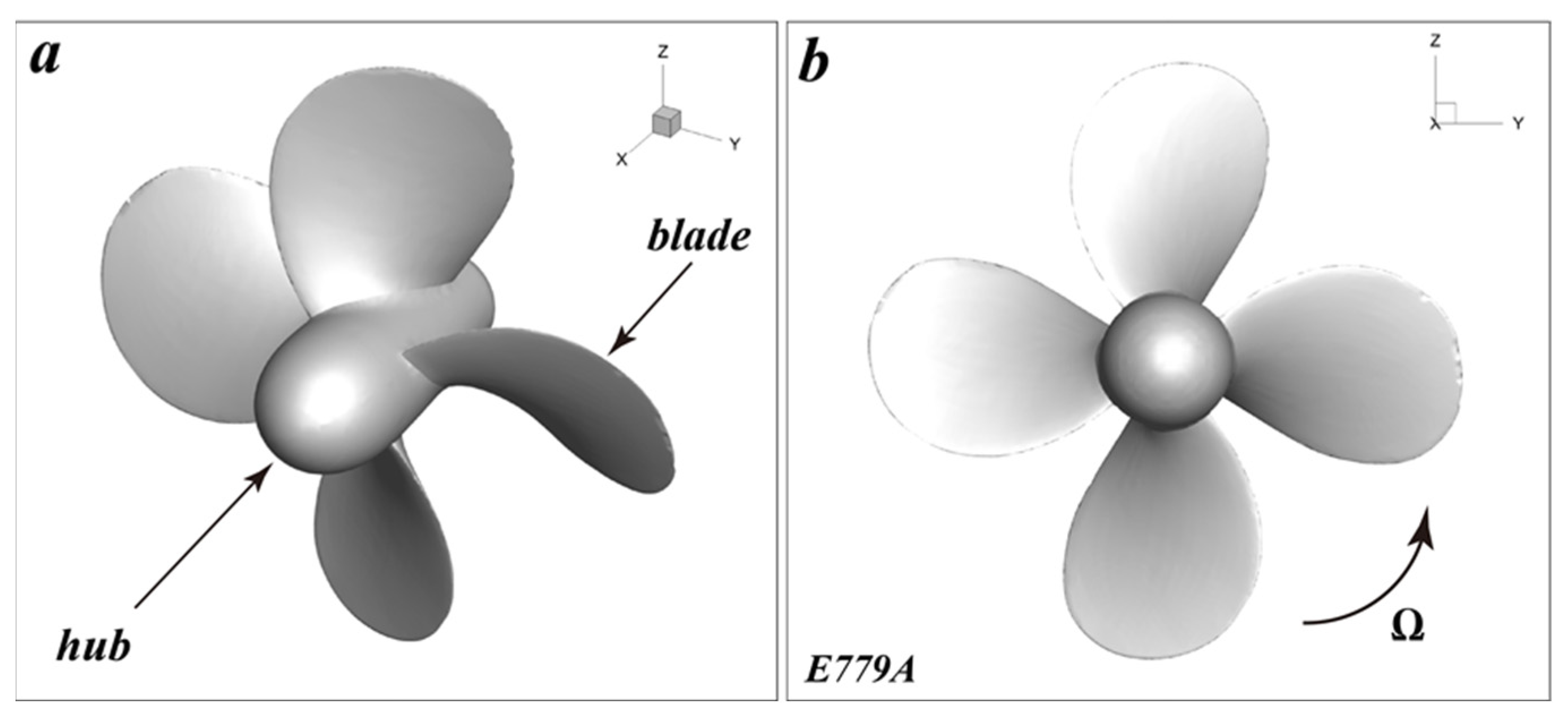
2. Research Model
3. Numerical Simulation
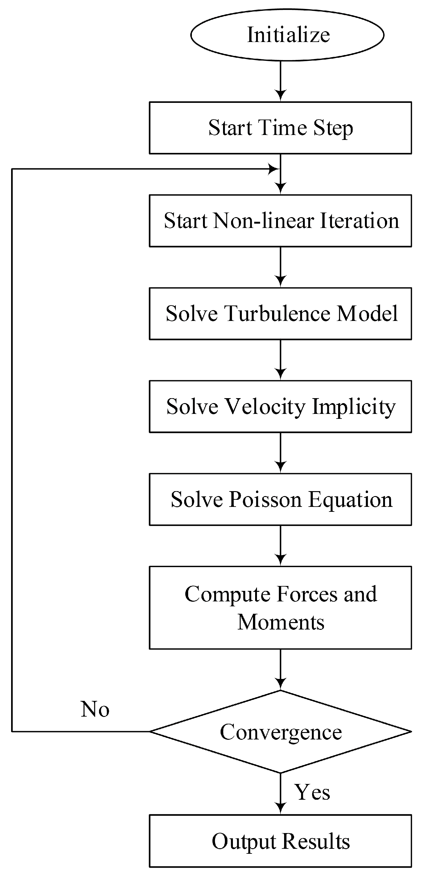
3.1. Numerical Method
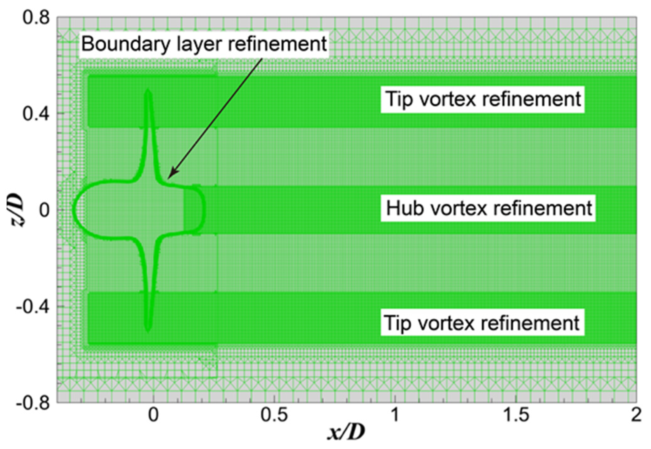
3.2. Computational Domain and Mesh Details
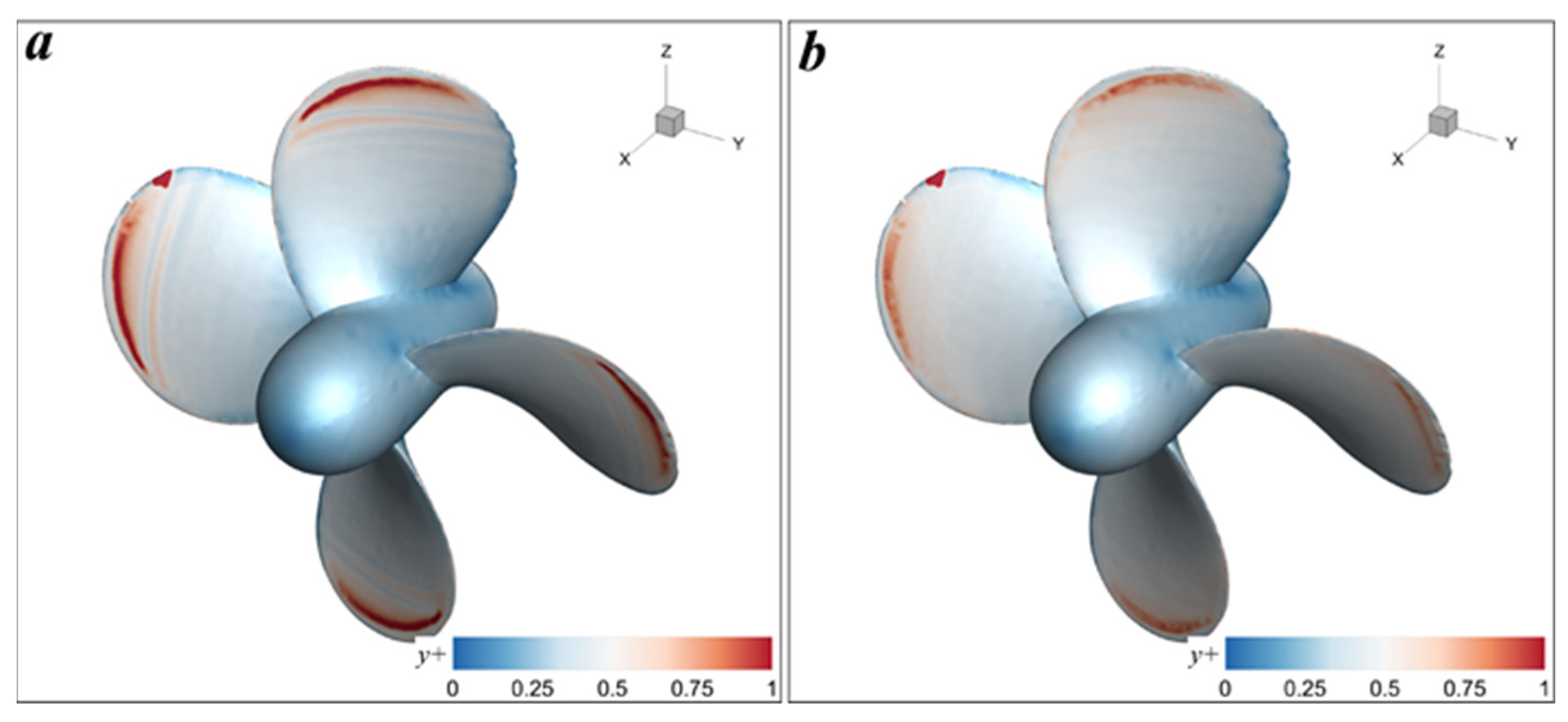
3.3. Numerical Validation
4. Results and Analysis
5. Conclusions
Author Contributions
Funding
Institutional Review Board Statement
Informed Consent Statement
Data Availability Statement
Conflicts of Interest
References
- Deng, R.; Zhang, Z.; Luo, F.; Sun, P.; Wu, T. Investigation on the Lift Force Induced by the Interceptor and Its Affecting Factors: Experimental Study with Captive Model. J. Mar. Sci. Eng. 2022, 10, 211. [Google Scholar] [CrossRef]
- Wang, L.Z.; Guo, C.Y.; Su, Y.M.; Wu, T.C. A numerical study on the correlation between the evolution of propeller trailing vortex wake and skew of propellers. Int. J. Nav. Archit. Ocean. Eng. 2018, 10, 212–224. [Google Scholar] [CrossRef]
- Sasmal, A.; De, S. Wave interaction with a pair of thick barriers over a pair of trenches. Ships Offshore Struct. 2022, 17, 2031–2044. [Google Scholar] [CrossRef]
- Das, A.; De, S.; Mandal, B.N. Radiation of water waves by a heaving submerged disc in a three-layer fluid. J. Fluids Struct. 2022, 111, 103575. [Google Scholar] [CrossRef]
- Sasmal, A.; De, S. Energy dissipation and oblique wave diffraction by three asymmetrically arranged porous barriers. Ships Offshore Struct. 2022, 17, 105–115. [Google Scholar] [CrossRef]
- Sun, C.; Wang, L. Modal analysis of propeller wake dynamics under different inflow conditions. Phys. Fluids 2022, 34, 125109. [Google Scholar] [CrossRef]
- Wang, H.; Hou, Y.; Xiong, Y.; Liang, X. Research on multi-interval coupling optimization of ship main dimensions for minimum EEDI. Ocean Eng. 2021, 237, 109588. [Google Scholar] [CrossRef]
- Di Mascio, A.; Dubbioso, G.; Muscari, R. Vortex structures in the wake of a marine propeller operating close to a free surface. J. Fluid Mech. 2022, 949, A33. [Google Scholar] [CrossRef]
- Zhao, D.; Guo, C.; Su, Y.; Wang, L.; Wang, C. Numerical study on the unsteady hydrodynamic performance of a four-propeller propulsion system undergoing oscillatory motions. J. Coast. Res. 2017, 33, 347–358. [Google Scholar] [CrossRef]
- Sun, P.; Pan, L.; Liu, W.; Zhou, J.; Zhao, T. Wake Characteristic Analysis of a Marine Propeller under Different Loading Conditions in Coastal Environments. J. Coast. Res. 2022, 38, 613–623. [Google Scholar] [CrossRef]
- Zhou, J.; Sun, P.; Pan, L. Modal Analysis of the Wake Instabilities of a Propeller Operating in Coastal Environments. J. Coast. Res. 2022, 38, 1163–1171. [Google Scholar] [CrossRef]
- Felli, M. Underlying mechanisms of propeller wake interaction with a wing. J. Fluid Mech. 2021, 908, A10. [Google Scholar] [CrossRef]
- Capone, A.; Di Felice, F.; Pereira, F.A. On the flow field induced by two counter-rotating propellers at varying load conditions. Ocean Eng. 2021, 221, 108322. [Google Scholar] [CrossRef]
- Wang, L.; Guo, C.; Wang, C.; Xu, P. Modified phase average algorithm for the wake of a propeller. Phys. Fluids 2021, 33, 035146. [Google Scholar] [CrossRef]
- de Vries, R.; van Arnhem, N.; Sinnige, T.; Vos, R.; Veldhuis, L.L. Aerodynamic interaction between propellers of a distributed-propulsion system in forward flight. Aerosp. Sci. Technol. 2021, 118, 107009. [Google Scholar] [CrossRef]
- Wang, L.; Martin, J.E.; Felli, M.; Carrica, P.M. Experiments and CFD for the propeller wake of a generic submarine operating near the surface. Ocean Eng. 2020, 206, 107304. [Google Scholar] [CrossRef]
- Posa, A.; Broglia, R.; Felli, M.; Falchi, M.; Balaras, E. Characterization of the wake of a submarine propeller via large-eddy simulation. Comput. Fluids 2019, 184, 138–152. [Google Scholar] [CrossRef]
- Posa, A.; Broglia, R. Near wake of a propeller across a hydrofoil at incidence. Phys. Fluids 2022, 34, 065141. [Google Scholar] [CrossRef]
- Posa, A.; Broglia, R.; Balaras, E. The dynamics of the tip and hub vortices shed by a propeller: Eulerian and Lagrangian approaches. Comput. Fluids 2022, 236, 105313. [Google Scholar] [CrossRef]
- Shi, H.; Wang, T.; Zhao, M.; Zhang, Q. Modal analysis of non-ducted and ducted propeller wake under axis flow. Phys. Fluids 2022, 34, 055128. [Google Scholar] [CrossRef]
- Qin, D.; Huang, Q.; Pan, G.; Chao, L.; Luo, Y.; Han, P. Effect of the odd and even number of blades on the hydrodynamic performance of a pre-swirl pumpjet propulsor. Phys. Fluids 2022, 34, 035120. [Google Scholar] [CrossRef]
- Wang, L.; Liu, X.; Wu, T. Modal analysis of the propeller wake under the heavy loading condition. Phys. Fluids 2022, 34, 055107. [Google Scholar] [CrossRef]
- Wang, L.; Liu, X.; Wang, N.; Li, M. Modal analysis of propeller wakes under different loading conditions. Phys. Fluids 2022, 34, 065136. [Google Scholar] [CrossRef]
- Li, H.; Huang, Q.; Pan, G.; Dong, X. Wake instabilities of a pre-swirl stator pump-jet propulsor. Phys. Fluids 2021, 33, 085119. [Google Scholar] [CrossRef]
- Qin, D.; Huang, Q.; Pan, G.; Han, P.; Luo, Y.; Dong, X. Numerical simulation of vortex instabilities in the wake of a preswirl pumpjet propulsor. Phys. Fluids 2021, 33, 055119. [Google Scholar] [CrossRef]
- Wang, L.; Carrica, P.M.; Felli, M. Experimental and CFD Study of the Streamwise Evolution of Propeller Tip Vortices. In Proceedings of the 33rd Symposium on Naval Hydrodynamics, Osaka, Japan, 18–23 October 2020; pp. 1–18. [Google Scholar]
- Muscari, R.; Di Mascio, A.; Verzicco, R. Modeling of vortex dynamics in the wake of a marine propeller. Comput. Fluids 2013, 73, 65–79. [Google Scholar] [CrossRef]
- Di Mascio, A.; Muscari, R.; Dubbioso, G. On the wake dynamics of a propeller operating in drift. J. Fluid Mech. 2014, 754, 263–307. [Google Scholar] [CrossRef]
- Li, H.; Huang, Q.; Pan, G.; Dong, X.; Li, F. An investigation on the flow and vortical structure of a pre-swirl stator pump-jet propulsor in drift. Ocean Eng. 2022, 250, 111061. [Google Scholar] [CrossRef]
- Chen, G.; Li, X.B.; Liang, X.F. IDDES simulation of the performance and wake dynamics of the wind turbines under different turbulent inflow conditions. Energy 2022, 238, 121772. [Google Scholar] [CrossRef]
- Wang, L.; Wu, T.; Gong, J.; Yang, Y. Numerical simulation of the wake instabilities of a propeller. Phys. Fluids 2021, 33, 125125. [Google Scholar] [CrossRef]
- Di Felice, F.; Di Florio, D.; Felli, M.; Romano, G.P. Experimental investigation of the propeller wake at different loading conditions by particle image velocimetry. J. Ship Res. 2004, 48, 168–190. [Google Scholar] [CrossRef]
- Salvatore, F.; Testa, C.; Ianniello, S.; Pereira, F. Theoretical modelling of unsteady cavitation and induced noise. In Proceedings of the CAV 2006 Symposium, Wageningen, The Netherlands, 11–15 September 2006; pp. 1–13. [Google Scholar]
- Sezen, S.; Cosgun, T.; Yurtseven, A.; Atlar, M. Numerical investigation of marine propeller underwater radiated noise using acoustic analogy Part 2: The influence of eddy viscosity turbulence models. Ocean Eng. 2021, 220, 108353. [Google Scholar] [CrossRef]
- Wang, L.; Guo, C.; Su, Y.; Xu, P.; Wu, T. Numerical analysis of a propeller during heave motion in cavitating flow. Appl. Ocean Res. 2017, 66, 131–145. [Google Scholar] [CrossRef]
- Wang, L.; Guo, C.; Xu, P.; Su, Y. Analysis of the performance of an oscillating propeller in cavitating flow. Ocean Eng. 2018, 164, 23–39. [Google Scholar] [CrossRef]
- Wang, L.; Guo, C.; Xu, P.; Su, Y. Analysis of the wake dynamics of a propeller operating before a rudder. Ocean Eng. 2019, 188, 106250. [Google Scholar] [CrossRef]
- Wang, L.; Wu, T.; Gong, J.; Yang, Y. Numerical analysis of the wake dynamics of a propeller. Phys. Fluids 2021, 33, 095120. [Google Scholar] [CrossRef]
- Posa, A.; Balaras, E. A numerical investigation of the wake of an axisymmetric body with appendages. J. Fluid Mech. 2016, 792, 470–498. [Google Scholar] [CrossRef]
- Wang, C.; Li, P.; Guo, C.; Wang, L.; Sun, S. Numerical research on the instabilities of CLT propeller wake. Ocean Eng. 2022, 243, 110305. [Google Scholar] [CrossRef]
- Kumar, P.; Mahesh, K. Large eddy simulation of propeller wake instabilities. J. Fluid Mech. 2017, 814, 361–396. [Google Scholar] [CrossRef]
- Andredaki, M.; Georgoulas, A.; Marengo, M. Numerical investigation of quasi-sessile droplet absorption into wound dressing capillaries. Phys. Fluids 2020, 32, 092112. [Google Scholar] [CrossRef]
- Nguyen, V.B.; Do, Q.V.; Pham, V.S. An OpenFOAM solver for multiphase and turbulent flow. Phys. Fluids 2020, 32, 043303. [Google Scholar] [CrossRef]
- Wang, L.; Guo, C.; Wan, L.; Su, Y. Numerical analysis of propeller during heave motion near a free surface. Mar. Technol. Soc. J. 2017, 51, 40–51. [Google Scholar]
- Wang, L.; Guo, C.; Su, Y.; Wu, T.; Wang, S. Numerical study of the viscous flow field mechanism for a non-geosim model. J. Coast. Res. 2017, 33, 684–698. [Google Scholar]
- Wang, L.; Guo, C.; Su, Y.; Zhang, D. Numerical study of the propeller-induced exciting force under the open freedom condition. J. Harbin Eng. Univ. 2017, 38, 822–828. [Google Scholar]
- Wang, L.; Guo, C.; Su, Y. Numerical analysis of flow past an elliptic cylinder near a moving wall. Ocean Eng. 2018, 169, 253–269. [Google Scholar] [CrossRef]
- Gong, J.; Ding, J.; Wang, L. Propeller–duct interaction on the wake dynamics of a ducted propeller. Phys. Fluids 2021, 33, 074102. [Google Scholar] [CrossRef]
- Roache, P.J. Quantification of uncertainty in computational fluid dynamics. Annu. Rev. Fluid Mech. 1997, 29, 123–160. [Google Scholar] [CrossRef]


| Quantity | Units | Value |
|---|---|---|
| Propeller diameter | mm | 227.27 |
| Number of blades | - | 4 |
| Pitch ratio | - | 1.11 |
| Hub diameter | mm | 45.53 |
| Hub ratio | - | 0.2 |
| Rake (forward) | - | 4°35′ |
| Expanded area ratio | - | 0.689 |
| Chord at 0.7R | mm | 86 |
| Load | Medium | Fine | E | Extr. | UN (%) |
|---|---|---|---|---|---|
| J = 0.38 | |||||
| Kt | 0.4015 | 0.3969 | 4.6 × 10⁻³ | 0.3923 | 1.17 |
| J = 0.65 | |||||
| Kt | 0.273 | 0.2767 | −3.7 × 10⁻³ | 0.2804 | 1.32 |
Disclaimer/Publisher’s Note: The statements, opinions and data contained in all publications are solely those of the individual author(s) and contributor(s) and not of MDPI and/or the editor(s). MDPI and/or the editor(s) disclaim responsibility for any injury to people or property resulting from any ideas, methods, instructions or products referred to in the content. |
© 2023 by the authors. Licensee MDPI, Basel, Switzerland. This article is an open access article distributed under the terms and conditions of the Creative Commons Attribution (CC BY) license (https://creativecommons.org/licenses/by/4.0/).
Share and Cite
Yu, D.; Zhao, Y.; Li, M.; Liu, H.; Yang, S.; Wang, L. Numerical Analysis of Propeller Wake Evolution under Different Advance Coefficients. J. Mar. Sci. Eng. 2023, 11, 921. https://doi.org/10.3390/jmse11050921
Yu D, Zhao Y, Li M, Liu H, Yang S, Wang L. Numerical Analysis of Propeller Wake Evolution under Different Advance Coefficients. Journal of Marine Science and Engineering. 2023; 11(5):921. https://doi.org/10.3390/jmse11050921
Chicago/Turabian StyleYu, Duo, Yu Zhao, Mei Li, Haitian Liu, Suoxian Yang, and Liang Wang. 2023. "Numerical Analysis of Propeller Wake Evolution under Different Advance Coefficients" Journal of Marine Science and Engineering 11, no. 5: 921. https://doi.org/10.3390/jmse11050921
APA StyleYu, D., Zhao, Y., Li, M., Liu, H., Yang, S., & Wang, L. (2023). Numerical Analysis of Propeller Wake Evolution under Different Advance Coefficients. Journal of Marine Science and Engineering, 11(5), 921. https://doi.org/10.3390/jmse11050921