Influence of Axial Matching between Inducer and Impeller on Energy Loss in High-Speed Centrifugal Pump

Abstract

Studying the axial matching between the inducer and impeller is crucial for optimizing the structure of centrifugal pumps. In this paper, the SST k-ω turbulence model is used to analyze the influence of three axial positions on the internal flow and the energy loss of a centrifugal pump. Additionally, the entropy generation method is used to evaluate the energy loss in the pump. Three sets of inducer design schemes are selected based on the ratio of the distance from the trailing edge of the inducer to the impeller inlet and the impeller inlet diameter, which are λ = 0.6, λ = 0.9 (original scheme), and λ = 1.2, respectively. The results indicate that changing the axial position of the inducer between λ = 0.6 and λ = 1.2 has only a negligible effect on the overall performance of the centrifugal pump. At flow rates of 0.6Q_d and 1.0Q_d, the inlet pressure coefficient of λ₂ is significantly lower compared to λ₁ and λ₃. As the flow rate increases, the pressure coefficient difference between the inlet and outlet in the inducer decreases, which leads to a more uniform streamline distribution and better development of the vortex in the flow channel. The energy loss in the inducer mainly occurs at the rim, the trailing edge, and outlet near the wall. As the flow rate increases, the entropy generation rate at the inducer rim decreases slightly and remains around 1000 W·m⁻³·K⁻¹. At flow rates of 1.0Q_d and 1.2Q_d, the energy loss in the impeller reduces as the axial distance increases, with the exception of the flow rate 0.6Q_d.

1. Introduction

Centrifugal pumps are utilized across various industries, including agriculture (for irrigation), water conservancy and hydropower, petrochemical, aerospace, metallurgy, and light industry. Due to the rapid advances in technology, research on energy-saving, efficient, stable, and reliable operation has become especially imperative. High efficiency helps to reduce energy consumption, reduce operating costs, and achieve dual economic and environmental benefits.

During the operation of a centrifugal pump, many unstable structures will be generated inside, such as backflow and flow separation. These flows have an impact on the performance of the pump, resulting in pressure pulsation and energy loss. Therefore, analyzing the internal flow and energy loss of the centrifugal pump is crucial.

Many studies have analyzed the internal flow structure of centrifugal pumps by numerical simulation. Gao et al. [1] described the formation and collapse of the separation vortex in the impeller, and revealed the law of the generation and development of the high pressure zone in the volute. Zhang et al. [2] showed that there are multi-scale distributions in the internal flow structure of centrifugal pumps, and the flow energy distribution in centrifugal pumps with better hydraulic performance is more concentrated in high-order and small-scale flow structures. Zhang et al. [3] discussed the influence of flow conditions on the liquid flow mechanism in the pump chamber and found that the vortex in the pump chamber is mainly concentrated near the volute and hub.

Many scholars have studied the geometric parameter structure to optimize the performance of the centrifugal pump. Zhang et al. [4] analyzed the hydraulic performance and dynamic characteristics of the centrifugal pump and indicated the pump has better hydraulic behavior when the volute tongue is right in the middle of the two vanes. Mihalic et al. [5] improved the performance of a centrifugal pump by adding a vortex rim on the back of the centrifugal rotor, and increased the stability of the pump when pumping a liquid and gas mixture. Shigemitsu et al. [6] found that when the centrifugal pump has splitter blades, the flow condition at the rotor outlet becomes uniform, the recirculation zone is suppressed, the volute efficiency is improved, and the vortex loss is reduced. Shen et al. [7] designed an innovative structure of longitudinal grooves on the volute casing and found that the modified volute pump can suppress and eliminate the unstable flow in the impeller channel and volute. Wang et al. [8] showed that with the T-shaped blade, the hydraulic loss can be reduced, the Euler head can be increased, and the external characteristics can be improved. Many scholars also use artificial intelligence algorithms to optimize the structure of centrifugal pumps. Wang et al. [9] applied artificial intelligence algorithms to consider various models for pump design, and the results showed that the performance of the pump had been improved. Nguyen et al. [10] established several design models by selecting the cross-sectional dimensions, tongue length, and tongue’s angle, and used an optimization algorithm to assist in the design, solving the optimization design problem of the pump.

The energy loss in the internal flow characteristics of a centrifugal pump was investigated. Jia et al. [11] analyzed how a combination of the entropy generation rate and vibration energy distribution changed the rules of flow loss and the vibration energy with the flow condition of the pump. Qian et al. [12] found that an uneven energy distribution brings extra energy loss and hydro-induced vibration, so attention should be paid to the circumferential distribution uniformity at impeller outlet. Zhao et al. [13] analyzed that the internal power loss of the centrifugal pump mainly occurs on the volute and impeller, and in some conditions, the flow separation and rotating stall cause the internal energy dissipation of the impeller. Yang et al. [14] analyzed the entropy generation analysis of each component of the pump and revealed that the clocking effect on the pump performance mainly originates from the turbulent dissipation in the impeller and the diffuser. Guan et al. [15] used the entropy generation theory to visualize the energy loss and found that the change of the vortex in the tongue and the outlet area will cause a significant change in the energy loss of the volute. Yuan et al. [16] used a variety of eddy identification methods and entropy generation analyses, and found that vorticity dominated by shear was the key factor to promote energy dissipation.

Although some progress has been made in the study of the internal flow and energy loss in centrifugal pumps, further research is required to match the different axial positions of the inducer and impeller. Moreover, studying the axial matching of the inducer and impeller contributes to the optimal design of inducer-equipped centrifugal pumps, as it enables them to achieve higher efficiency and longer service life. This article is based on SST k-ω turbulence model, numerical simulation, and experimentation to analyze the flow field in high-speed centrifugal pumps with inducers, and to evaluate the relationship between inducer and impeller axial matching for internal flow and energy loss at various operating conditions.

2. Research Object

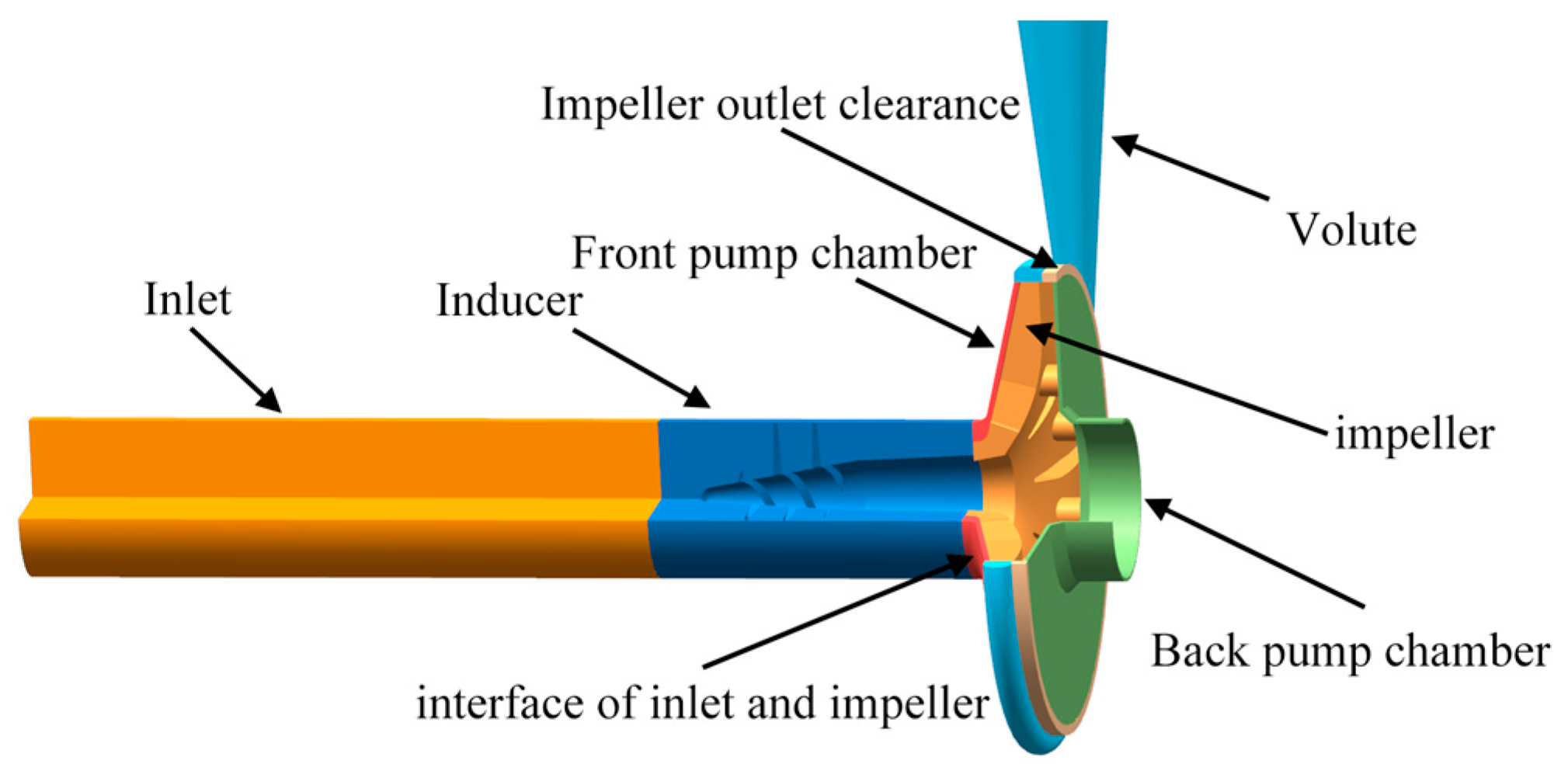
2.1. Object Model

The main manufacturing material of the pump is 0Cr18Ni9, and the fluid medium inside the centrifugal pump is water. The inlet diameter of the centrifugal pump is 40 mm, the outlet diameter is 32 mm, and the impeller diameter is 113 mm. The main components include the inducer with two blades and a semi-open impeller with eight straight blades. The primary design parameters are as follows: flow rate Q = 4 m³·h⁻¹, head H = 125 m, rotating speed n = 7081 r·min⁻¹. The specific speed of the model pump is 23.6, with its flow channel model depicted in Figure 1. The main parameters of the inducer are shown in

Table 1. Main parameters of the model inducer.

Parameter	Value
Design rotational speed (r/min)	7081
Number of blades (sheet)	2
Tip diameter (mm)	39.4
Sweepback angle of leading edge (deg)	120
Inlet hub diameter (mm)	8
Outlet hub diameter (mm)	20
Axial length (mm)	26.4

.

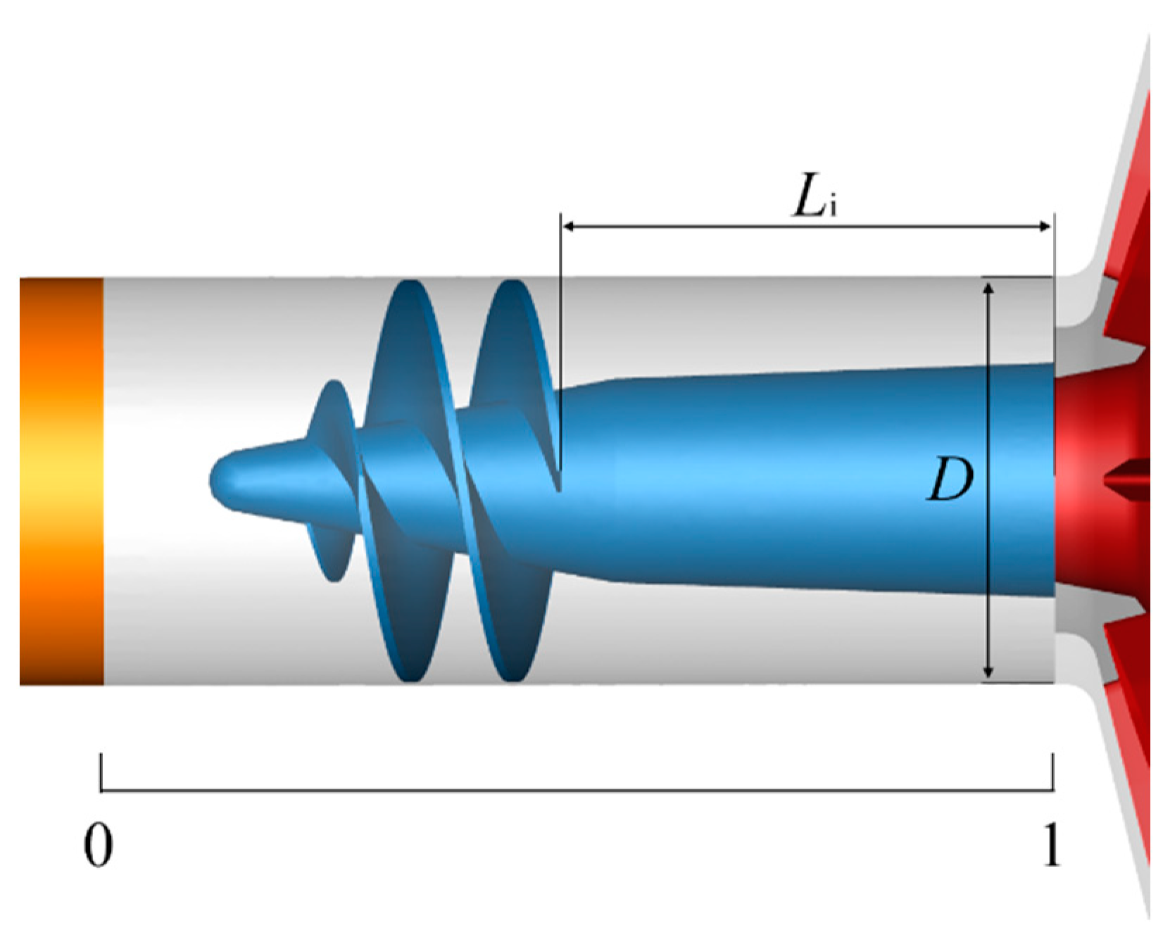
2.2. Scheme Design

The effect of the axial distance L_i from the trailing edge of the inducer to the impeller inlet on the internal flow of centrifugal pumps are studied at different flow rates. As shown in Figure 2, L_i has dimensions of 24.28 mm, 35.28 mm, and 48.28 mm, respectively, and the impeller inlet diameter D₁ is 40 mm. The ratio of L_i and D₁ is defined as λ, where λ₁ = 0.6, λ₂ = 0.9, and λ₃ = 1.2.

$${\lambda }_i=\frac{L_i}{D_1}(i=1,2,3)$$

(1)

2.3. Boundary Condition

A constant pressure is specified in the inlet. The mass flow is set in the outlet, and the overall flow rate of the centrifugal pump is controlled by adjusting the outlet flow rate. No slip wall condition is assumed on the solid wall. In centrifugal pumps, with the exception of rotating components such as the inducer and impeller, all other components remain stationary.

3. Numerical Method

3.1. Governing Equation

3.1.1. Mass-Conservation Equation

The mass conservation equation is also called the continuity equation. The change of the total amount of a certain conserved quantity in any region is equal to the amount entering or leaving from the boundary.

$$\frac{\partial \rho }{\partial t}+\frac{\partial (\rho u)}{\partial x}+\frac{\partial (\rho v)}{\partial y}+\frac{\partial (\rho w)}{\partial z}=0$$

(2)

3.1.2. Momentum Conservation Equation

The momentum conservation equation is defined as the rate of change of momentum in any control element over time, which is equal to the sum of external forces acting on the element.

$$\frac{\partial (\rho u)}{\partial t}+u\frac{\partial u}{\partial x}+v\frac{\partial u}{\partial y}+w\frac{\partial w}{\partial z}=-\frac{\partial p}{\partial x}+\frac{\partial {\tau }_{xx}}{\partial x}+\frac{\partial {\tau }_{yx}}{\partial y}+\frac{\partial {\tau }_{zx}}{\partial z}+F_x$$

(3)

$$\frac{\partial (\rho v)}{\partial t}+u\frac{\partial v}{\partial x}+v\frac{\partial v}{\partial y}+w\frac{\partial v}{\partial z}=-\frac{\partial p}{\partial x}+\frac{\partial {\tau }_{xy}}{\partial x}+\frac{\partial {\tau }_{yy}}{\partial y}+\frac{\partial {\tau }_{zy}}{\partial z}+F_y$$

(4)

$$\frac{\partial (\rho w)}{\partial t}+u\frac{\partial w}{\partial x}+v\frac{\partial w}{\partial y}+w\frac{\partial w}{\partial z}=-\frac{\partial p}{\partial x}+\frac{\partial {\tau }_{xz}}{\partial x}+\frac{\partial {\tau }_{yz}}{\partial y}+\frac{\partial {\tau }_{zz}}{\partial z}+F_z$$

(5)

In the above equations, ${\tau }_{xx}$, ${\tau }_{yy}$, and ${\tau }_{zz}$ are the viscous forces $\tau$ of components in the x, y, and z directions; $F_x$, $F_y$, and $F_z$ are the volume forces acting on the microelement in the x, y, and z directions; P is the pressure.

3.2. Turbulence Mode

The SST k-ω turbulence model is a hybrid model with the accuracy of both the k-ω model for viscous flow calculations in the near-wall region and the k-ε model for free flow calculations in the mainstream region. This model considers turbulent shear stress transfer, which results in an accurate simulation of flow separation and helps predict vortex structures near the blade’s wall. However, the SST k-ω turbulence model has some limitations in the numerical simulation, in terms of a high Reynolds number. Since the research objects considered in this paper have low Reynolds numbers, their accuracies remain unaffected.

The transport equation expressions for the turbulent kinetic energy k and ω specific dissipation rate of the SST k-ω model are given by:

$$\frac{\partial k}{\partial t}+{\overline{u}}_j\frac{\partial k}{\partial x_j}=\frac{\partial }{\partial x_j}\left[\left(v+{\sigma }_k{v}_t\right)\frac{\partial k}{\partial x_j}\right]+p+\beta \ast k\omega$$

(6)

$$\frac{\partial \omega }{\partial t}+{\overline{u}}_j\frac{\partial \omega }{\partial x_j}=\frac{\partial }{\partial x_j}\left[\left(v+{\sigma }_{\omega }{v}_t\right)\frac{\partial \omega }{\partial x_j}\right]+\alpha S^2-\beta {\omega }^2+2\left(1-F_1\right){\sigma }_{\omega 2}\frac{1}{\omega }\frac{\partial k}{\partial x_j}\frac{\partial \omega }{\partial x_j}$$

(7)

$$v_t=\frac{a_{1}k}{\max \left(a_1\omega ,\Omega F_2\right)}$$

(8)

where ${\sigma }_k=\frac{1}{F_1/{\sigma }_{k1}+\left(1-F_1\right)/{\sigma }_{k2}}$; and ${\sigma }_{\omega }=\frac{1}{F_1/{\sigma }_{\omega 1}+\left(1-F_1\right)/{\sigma }_{\omega 2}}$.

3.3. Entropy Generation Theory

Entropy generation theory is widely used to evaluate the sources of irreversible energy dissipation in systems. In a centrifugal pump, entropy generation is mainly caused by the viscous force of the fluid converting mechanical energy into internal energy dissipation. For turbulent flow, the entropy generation rate can be divided into two parts: one part is caused by time-averaged motion, the other part is caused by turbulent dissipation resulting from the pulsating velocity. The entropy generation rate (EGR) can be calculated by:

$${{\dot{S}}_D}^{‴}={{\dot{S}}_{\overline{D}}}^{‴}+{{\dot{S}}_{D^{\prime }}}^{‴}$$

(9)

$${{\dot{S}}_{\overline{D}}}^{‴}=\frac{\mu }{\overline{T}}\left[2\left\{{\left(\frac{\partial \overline{u}}{\partial x}\right)}^2+{\left(\frac{\partial \overline{v}}{\partial y}\right)}^2+{\left(\frac{\partial \overline{w}}{\partial z}\right)}^2\right\}+{\left(\frac{\partial \overline{u}}{\partial y}+\frac{\partial \overline{v}}{\partial x}\right)}^2+{\left(\frac{\partial \overline{u}}{\partial z}+\frac{\partial \overline{w}}{\partial x}\right)}^2+{\left(\frac{\partial \overline{v}}{\partial z}+\frac{\partial \overline{w}}{\partial y}\right)}^2\right]$$

(10)

$${{\dot{S}}_{D^{\prime }}}^{‴}=\frac{\mu }{\overline{T}}\left[2\left\{\overline{{\left(\frac{\partial u^{\prime }}{\partial x}\right)}^2}+\overline{{\left(\frac{\partial v^{\prime }}{\partial y}\right)}^2}+\overline{{\left(\frac{\partial w^{\prime }}{\partial z}\right)}^2}\right\}+\overline{{\left(\frac{\partial u^{\prime }}{\partial y}+\frac{\partial v^{\prime }}{\partial x}\right)}^2}+\overline{{\left(\frac{\partial u^{\prime }}{\partial z}+\frac{\partial w^{\prime }}{\partial x}\right)}^2}+\overline{{\left(\frac{\partial v^{\prime }}{\partial z}+\frac{\partial w^{\prime }}{\partial y}\right)}^2}\right]$$

(11)

$${{\dot{S}}_{D^{\prime }}}^{‴}=\frac{\rho \epsilon }{T}$$

(12)

where ${{\dot{S}}_{\overline{D}}}^{‴}$ denotes the direct dissipative entropy generation rate, and ${{\dot{S}}_{D^{\prime }}}^{‴}$ denotes the indirect dissipative entropy generation rate.

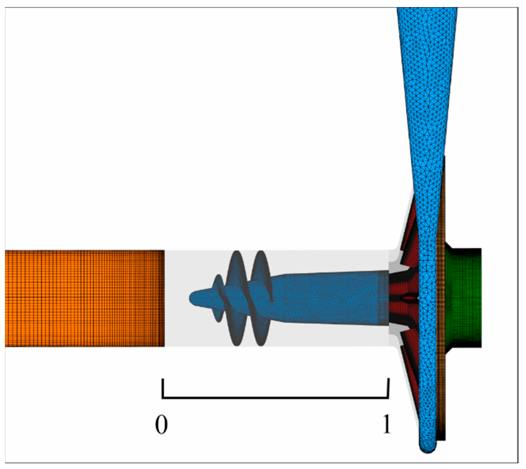
3.4. Numerical Setup and Grid Validation

Considering the complexity and irregularity of the pump structure, the entire computational fluid domain is meshed by a well-adapted nonstructural tetrahedral grid, including the inducer and the volute, and structural meshing for inlet, impeller, front pump chamber and back pump chamber. The grid of the main fluid domains is shown in Figure 3. Six different sets of full flow field grid numbers are used to check the grid-independence. The results are shown in Figure 4. When the number of grids reaches 5.19 million, the variation error of the calculated head of the centrifugal pump is less than 1% as the number of grids increases. Finally, the computational accuracy and computational efficiency are considered comprehensively, and a full flow field computational grid with the number of 5,198,692 is used in this paper.

4. Results and Discussion

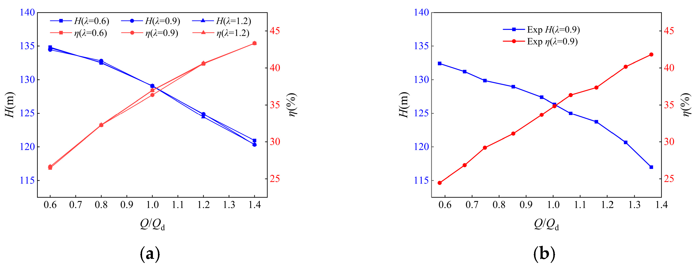
4.1. Performance Curve of High-Speed Pump

In order to improve the overall performance of the model pump, an increased flow coefficient design method was used in the design, so the maximum efficiency value is not at the design operating point. The performance curve of the centrifugal pump with the inducer obtained from the numerical simulation is shown in Figure 5a. The heads of scheme λ₁, λ₂, and λ₃ are 129.092 m, 129.049 m, and 129.065 m, and the efficiencies are 36.96%, 36.35%, and 36.99%, respectively, at a flow rate of 1.0Q_d. The Experimental performance curve is shown in Figure 5b. The numerical simulation results are in good agreement with the experimental results, with the head error less than 3% and the efficiency error less than 7%. The results show that the inducer at different axial positions between λ = 0.6 and λ = 1.2 does not have a large impact on the head and efficiency of the centrifugal pump, which is because the most important working component in the pump is the impeller.

4.2. The Variation Law of Inducer Streamline and Turbulent Kinetic Energy

In order to study the influence of different axial positions on the flow characteristics inside the inducer, the distribution of the static pressure coefficient (C_p) in the inducer basin is analyzed. The static pressure coefficient is a dimensionless number that describes the relative pressure across the entire flow field in fluid dynamics. It can reflect the pressure fluctuations generated by the fluid flowing in the flow channel. It is defined as

$$C_{\mathrm{p}}=\frac{P-P_{\mathrm{out}}}{\frac{1}{2}\rho U_T^2}$$

(13)

where P is the average static pressure value of a section, P_out is the average static pressure value of the inducer outlet section, ρ is the density of the fluid medium, and U_T is the inducer blade tip speed.

As shown in Figure 2, the same area in the inducer domain without the inlet extension section is studied. Figure 6 shows the pressure distribution on the radial surface of the inducer, and it can be seen from the figure that there is an obvious low-pressure area at the leading edge of the inducer, and the high-pressure area appears at the trailing edge of the inducer near the wall. With the increase of axial distance, the pressure distribution at the outlet is more uniform. Figure 7 shows the static pressure coefficient distribution of the inducer domain from the inlet to the outlet in three axial positions; it can be seen from the figure that the pressure coefficient at the inlet of the inducer increases gradually with the increase of the flow rate. The pressure coefficient from the inlet to the rim section of the inducer remains constant. At 0.6Q_d and 1.0Q_d, the inlet pressure coefficient of λ₂ is significantly lower than λ₁ and λ₃. At the 1.0Q_d and 1.2Q_d flow rates, the pressure coefficient at the rim decreases first and then increases. At 0.6Q_d, the highest static pressure coefficients of the fluid at the trailing edges of λ₁, λ₂, and λ₃ are 0.01094, 0.01276, and 0.014006, respectively. At 1.0Q_d, the highest static pressure coefficient of the fluid at the trailing edges of λ₁, λ₂, and λ₃ are 0.00926, 0.01272, and 0.00840. At 1.2Q_d, the highest static pressure coefficients of the fluid at the trailing edges of λ₁, λ₂, and λ₃ are 0.01191, 0.01210, and 0.01092. After that, the inducer works on the fluid to gradually increase the pressure coefficient, the pressure coefficient after the trailing edge again decreases until the fluid reaching the outlet remains unchanged. At the 0.6Q_d flow rate, the pressure coefficient at the trailing edge increases with the increase λ, but the pressure coefficient becomes uniform when it reaches the outlet.

Turbulent kinetic energy indicates the degree of the turbulent vortex; the higher the value of turbulent energy, representing the more violent the fluid velocity pulsation, the greater energy loss of the fluid flow. Figure 8a–c show the turbulent kinetic energy distribution and flow line of the radial surface of the inducer. It can be seen from the figures that the turbulent kinetic energy is higher in the region of the leading edge of the inducer. The reason for the large turbulence kinetic energy is that the main stream is at the entrance and the blade is at a certain angle of attack. However, as the flow rate increases, the turbulent kinetic energy gradually decreases. The greater the flow velocity, the greater the dynamic pressure, the lower the static pressure, and thus the strength of the backflow will decrease. The back flow vortex area of the inducer decreases with the increase of the flow rate, and the back flow area of the tip clearance of the inducer is the largest at 1.0Q_d. At the same flow rate, with the increase of λ, the streamline state from the trailing edge of the inducer to the outlet is better, and the vortex in the flow channel develops more fully. Increasing the axial distance of the inducer can result in a reduction of turbulent kinetic energy from the trailing edge to the outlet of the inducer, which can ultimately decrease flow resistance and energy loss in the fluid.

4.3. Analysis of the Distribution of Energy Loss in the Inducer

Figure 9 shows the entropy generation rate of the radial surface and the 3D profiles on the inducer at 1.0Q_d flow rate. It can be seen that the energy loss at the inducer mainly occurs at the rim near the wall, the trailing edge, and the outlet. The entropy generation rate at the rim is mainly influenced by the interaction of the backflow and shear stress, and the entropy generation rate at the trailing edge is mainly influenced by the backflow vortex and wake flow. The difference in energy loss at the inducer outlet is due to the influence of the interface of inducer and impeller. The entropy generation rate of λ₁ and λ₃ at the inducer outlet are lower than that of λ₂.

Figure 10a–c show the surface-average entropy generation rate in the axial direction of the inducer at 0.6Q_d, 1.0Q_d and 1.2Q_d, respectively. The entropy generation rate increases gradually at the inlet of the inducer, because the backflow vortex is generated at the leading edge. The entropy generation rate increases first and then decreases at the rim, while in the trailing edge of the inducer, it slightly increases and then decreases. When the fluid flows near the inducer outlet, the entropy generation rate increases again. At the 0.6Q_d flow rate, as shown in Figure 10a, the entropy generation rate gradually decreases with the increase of λ at the outlet of the inducer. At the 1.0Q_d flow rate, as shown in Figure 10b, the trend at the outlet is the same as at 0.6Q_d, but the difference in entropy generation rate becomes smaller for different axial distances. At the 1.2Q_d flow rate, as shown in Figure 10c, the entropic generation rate is very low, which is different from the entropy generation rate in the outlet at 0.6Q_d and 1.0Q_d, and there is no change in the three axial distances. With the increase of flow rate, the entropy generation rate at the inducer rim decreases slightly and remains near 1000 W·m⁻³·K⁻¹. The entropy generation rate at the trailing edge of the inducer increases with the increase of flow rate, resulting in more energy loss. The energy loss at the outlet of the inducer decreases with the increase of the flow rate. When the flow rate reaches 1.2Q_d, the rate of entropy generation rate decreases sharply.

It can be seen from Figure 9 and Figure 10 that the entropy generation mainly occurs near the wall, and there is little difference in the entropy production rate of each axial position when there is a large flow rate. Therefore, the near wall of 0.6Q_d and 1.0Q_d is analyzed. Figure 11 shows the entropy generation rate and velocity distribution in span = 0.95 of the inducer at different operating conditions. It can be seen from the figure that the entropy generation rate of the inducer domain mainly occurs in the region with large velocity gradient at the rim and outlet. The entropy generation rate will be higher at 0.6Q_d, and decreases gradually with increases of the flow rate. As the axial distance increases, the energy loss at the inducer outlet decreases, because more vortices are generated at small flow rates. By comparing the entropy generation rate distribution of cascades at different axial positions at the same flow rate, it was found that the entropy production rate at the rim does not change.

4.4. Analysis of the Distribution of Energy Loss in the Impeller

Figure 12 shows the entropy generation rate distribution of the interface of inducer and impeller with a 1.0Q_d flow rate. It can be seen from the figure that a large energy loss is generated near the wall, and the entropy generation area of the axial distance λ₂ is higher than λ₁ and λ₃. The entropy generation rate of λ₃ is obviously lower than that of λ₁ and λ₂. Figure 13 shows the area-average entropy generation rate of the interface of inducer and impeller. The energy loss at the 0.6Q_d flow rate is significantly larger than the other flow rates. As the flow rate increases, the entropy generation rate of the interface decreases first and then increases. With the exception of the 1.0Q_d flow rate, the entropy generation rate of λ₃ is significantly lower than that of λ₁ and λ₂ at other flow rates, because as the axial distance increases, the vortex at the outlet of the inducer becomes less and the streamline is more uniform.

Figure 14 shows the entropy generation rate distribution of the impeller at 1.0Q_d. From the figure, it can be seen that the distribution of the entropy generation rate of the impeller at three axial positions is the same, indicating that changing the axial distance of the inducer will not significantly affect the energy loss of the impeller. Figure 15 shows the volume-average entropy generation rate of the impeller. As the flow rate increases, the entropy generation rate at the impeller first decreases and then increases. At the 0.6Q_d flow rate, as the axial distance increases, the entropy generation rate gradually increases, which is due to the more unstable internal flow at small flow rates. At other flow rates, as the axial distance increases, the entropy generation rate gradually decreases, which is consistent with the trend in Figure 13.

5. Conclusions

The influence of three axial positions on the internal flow and energy loss of a centrifugal pump are investigated based on the SST k-ω turbulence model at different flow rates. The pressure, turbulent kinetic energy, and entropy generation rate are emphatically analyzed. Several conclusions can be drawn from this paper.

• Changing the axial position of the inducer between λ = 0.6 and λ = 1.2 will not have a significant impact on the overall performance of the centrifugal pump.
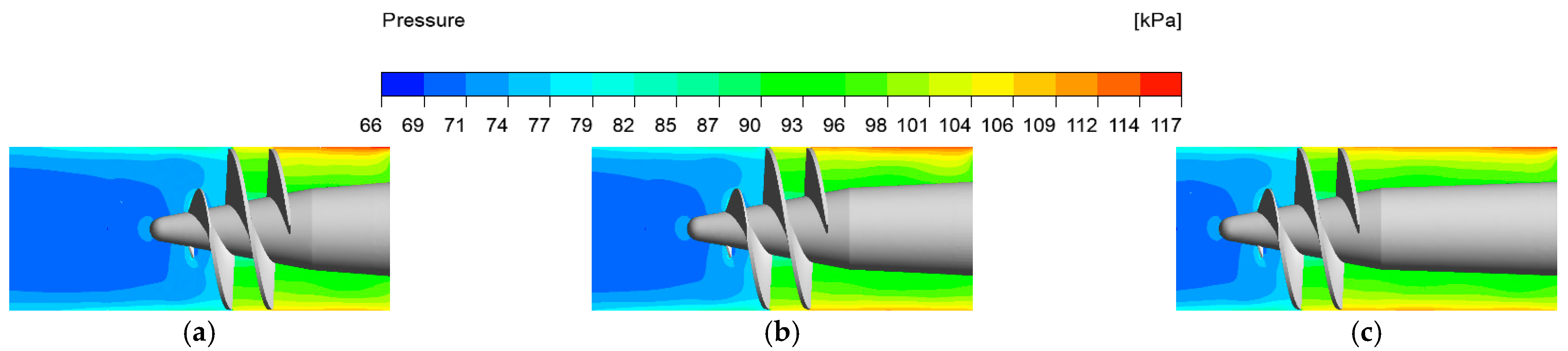
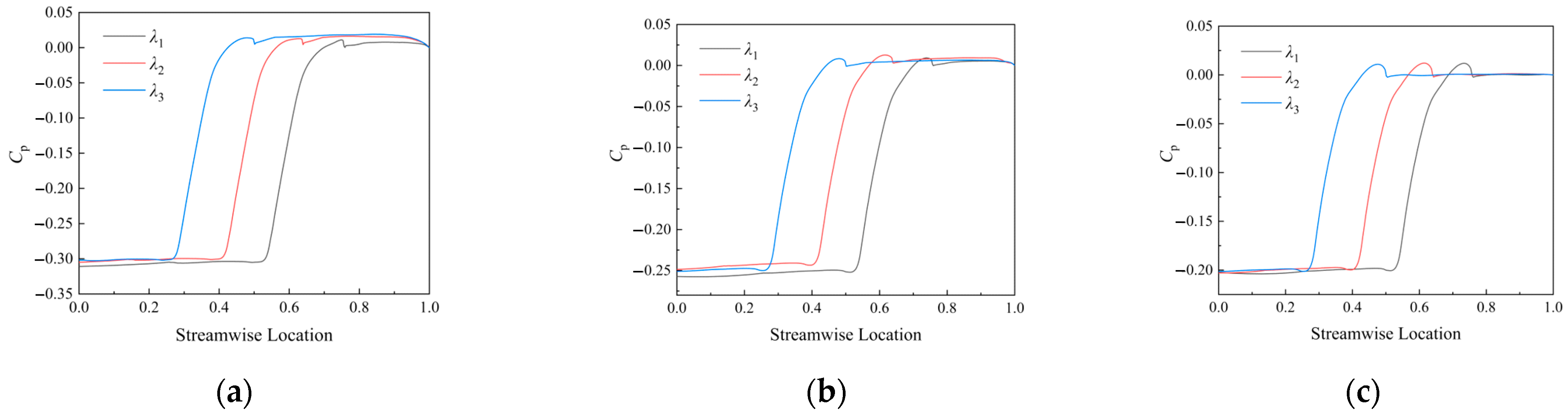
• After analyzing the pressure and turbulent kinetic energy of the inducer, it was found that at a 0.6Q_d flow rate, the pressure coefficient increases with the increase of λ at the inducer trailing edge, but the pressure coefficient becomes uniform upon reaching the outlet. There is almost no difference in pressure at the three axial positions at other flow rates. The turbulent kinetic energy in the inlet of the leading edge of the inducer is larger, and the turbulent kinetic energy here gradually decreases with the increase of the flow rate. At the same flow rate, as the axial distance increases, the streamline distribution from the trailing edge of the inducer to the outlet is more uniform, and the vortex in the flow channel develops more fully.
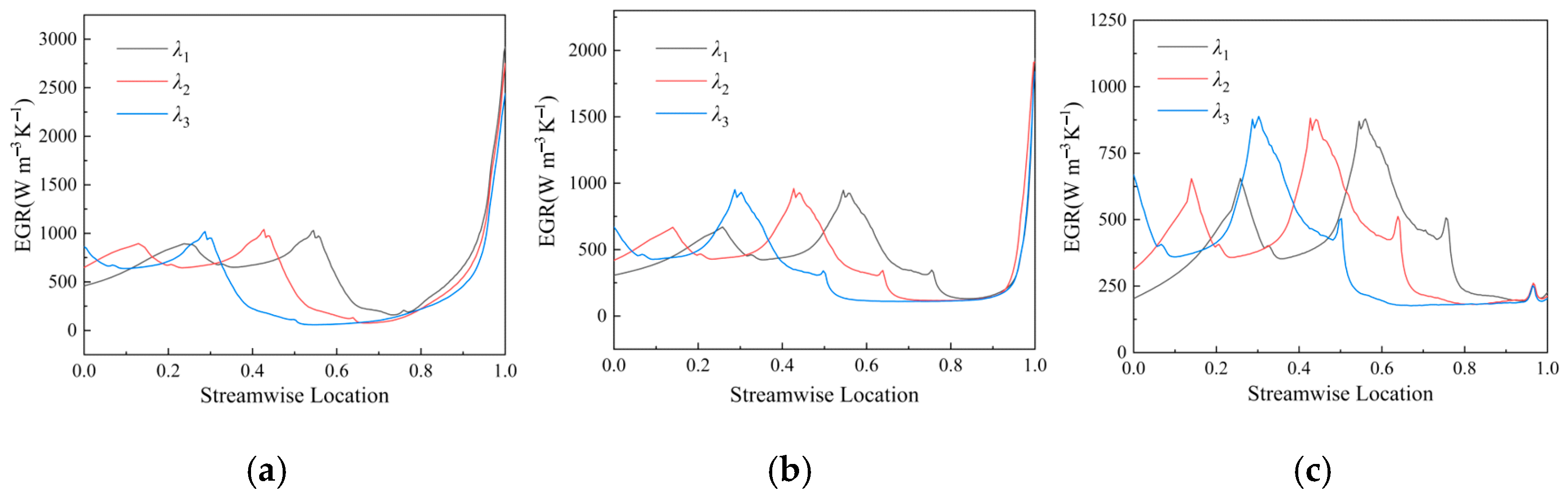
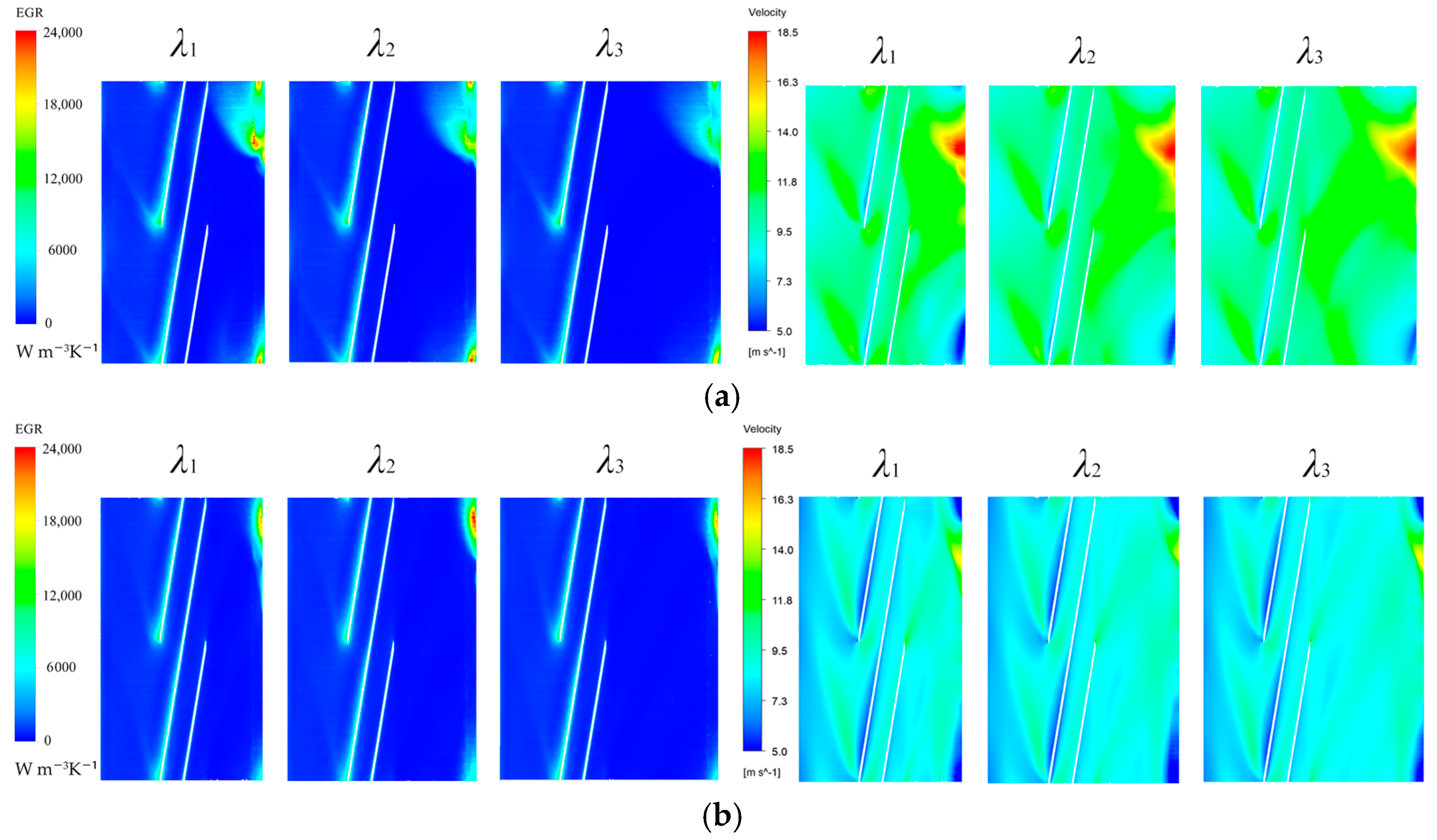
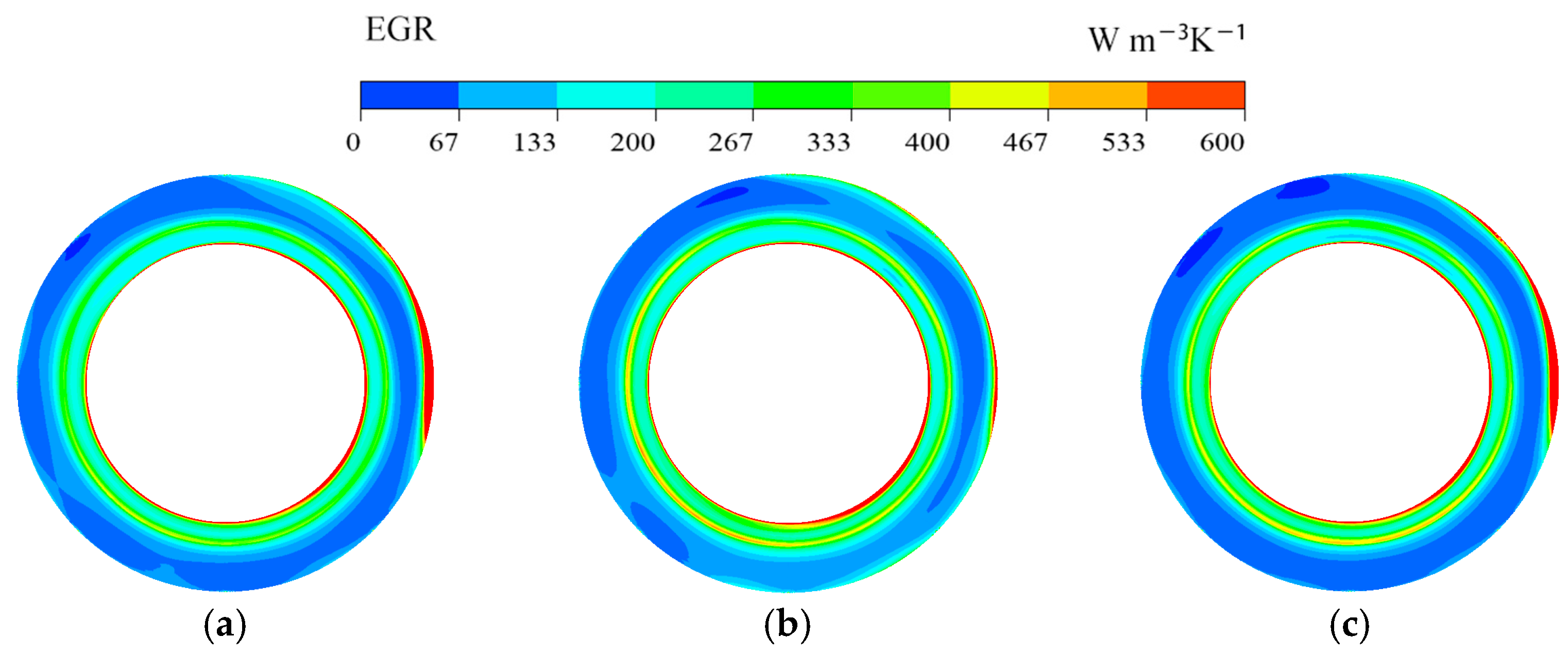
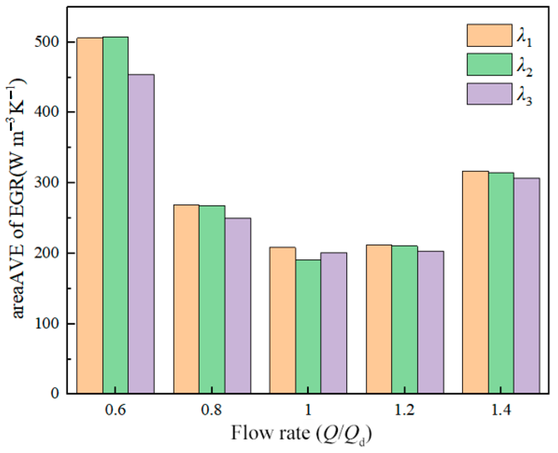
• The energy loss in the inducer mainly occurs at the rim, trailing edge, and outlet near the wall. The entropy generation rate at the trailing edge increases with the increase of the flow rate, resulting in more energy loss. The energy loss at the inducer outlet decreases as the flow rate increases. When the flow rate reaches 1.2Q_d, the entropy generation rate drops sharply.
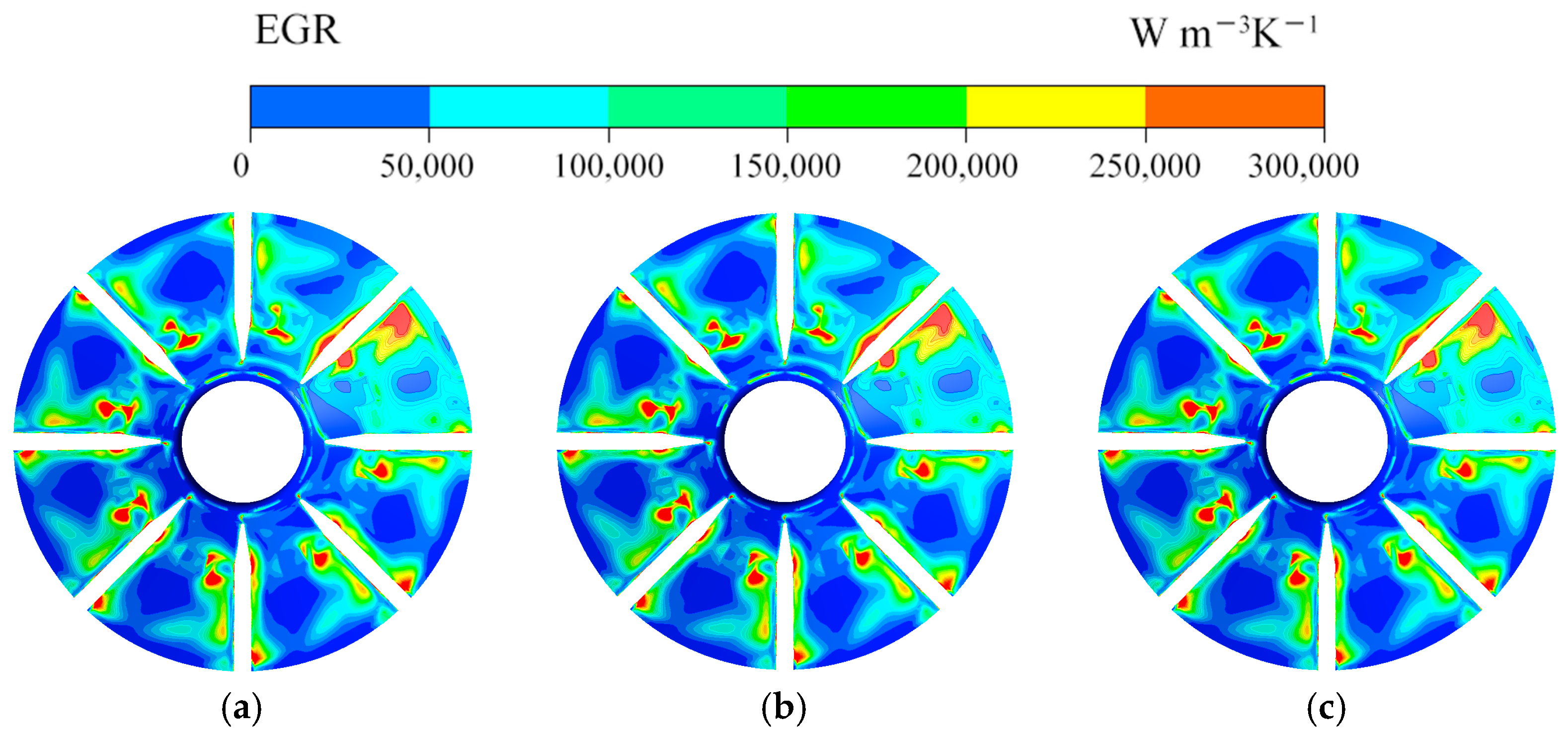
• The energy loss at the interface between the inducer and the impeller, as well as in the impeller, at a 0.6Q_d flow rate is significantly larger than at other flow rates. The entropy generation rate in the impeller decreases first and then increases with the increase of flow rate, and the entropy generation rate of the impeller gradually decreases with the increase of the axial distance, except for at a flow rate of 0.6Q_d.

References

- Gao, Q.; Ye, J.; Wang, B.; Zhao, J. Investigation of Unsteady Pressure Pulsation and Internal Flow in a Centrifugal Pump under Low Flow Rate. Int. J. Fluid Mach. Syst. 2019, 12, 189–199. [Google Scholar] [CrossRef]
- Zhang, Z.; Chen, H.; Yin, J.; Ma, Z.; Gu, Q.; Lu, J.; Liu, H. Unsteady flow characteristics in centrifugal pump based on proper orthogonal decomposition method. Phys. Fluids 2021, 33, 075122. [Google Scholar] [CrossRef]
- Zhang, H.; Dong, W.; Chen, D. Numerical analysis of the flow mechanism and axial force characteristics of the cavity in a centrifugal pump with a front inducer. J. Vibroeng. 2020, 22, 1210–1227. [Google Scholar] [CrossRef]
- Zhang, X.-Y.; Jiang, C.-X.; Lv, S.; Wang, X.; Yu, T.; Jian, J.; Shuai, Z.-J.; Li, W.-Y. Clocking effect of outlet RGVs on hydrodynamic characteristics in a centrifugal pump with an inlet inducer by CFD method. Eng. Appl. Comp. Fluid 2021, 15, 222–235. [Google Scholar] [CrossRef]
- Mihalic, T.; Kondic, Z.; Medic, S.; Kondic, V. Experimental and Numerical Investigation of Centrifugal Vortex Pump Operating Benefits for Energy Efficient Systems. Teh. Vjesn. 2020, 27, 1519–1523. [Google Scholar] [CrossRef]
- Shigemitsu, T.; Ogawa, Y.; Nakaishi, E. PIV Measurement of Internal Flow in Mini Centrifugal Pump. Int. J. Fluid Mach. Syst. 2019, 12, 251–260. [Google Scholar] [CrossRef]
- Shen, Z.; Chu, W.; Yan, S.; Chen, X.; Guo, Z.; Zhong, Y. Study of the performance and internal flow in centrifugal pump with grooved volute casing. Mod. Phys. Lett. B 2020, 34, 2050268. [Google Scholar] [CrossRef]
- Wang, L.-K.; Lu, J.-L.; Liao, W.-L.; Guo, P.-C.; Feng, J.-J.; Luo, X.-Q.; Wang, W. Numerical investigation of the effect of T-shaped blade on the energy performance improvement of a semi-open centrifugal pump. J. Hydrodyn. 2021, 33, 736–746. [Google Scholar] [CrossRef]
- Wang, C.N.; Yang, F.C.; Nguyen, V.T.T.; Vo, N.T.M. CFD Analysis and Optimum Design for a Centrifugal Pump Using an Effectively Artificial Intelligent Algorithm. Micromachines 2022, 13, 1208. [Google Scholar] [CrossRef] [PubMed]
- Nguyen, V.T.T.; Vo, T.M.N. Centrifugal Pump Design: An Optimization. Eurasia Proc. Sci. Technol. Eng. Math. 2022, 17, 136–151. [Google Scholar] [CrossRef]
- Jia, X.-Q.; Zhu, Z.-C.; Yu, X.-L.; Zhang, Y.-L. Internal unsteady flow characteristics of centrifugal pump based on entropy generation rate and vibration energy. Proc. Inst. Mech. Eng. Part E J. Process Mech. Eng. 2019, 233, 456–473. [Google Scholar] [CrossRef]
- Qian, B.; Chen, J.-P.; Wu, P.; Wu, D.-Z.; Yan, P.; Li, S.-Y. Investigation on inner flow quality assessment of centrifugal pump based on Euler head and entropy production analysis. In Proceedings of the 29th IAHR Symposium on Hydraulic Machinery and Systems (IAHR), Kyoto, Japan, 17–21 September 2018. [Google Scholar]
- Zhao, X.; Luo, Y.; Wang, Z.; Xiao, Y.; Avellan, F. Unsteady Flow Numerical Simulations on Internal Energy Dissipation for a Low-Head Centrifugal Pump at Part-Load Operating Conditions. Energies 2019, 12, 2013. [Google Scholar] [CrossRef]
- Yang, B.; Li, B.; Chen, H.; Liu, Z. Entropy production analysis for the clocking effect between inducer and impeller in a high-speed centrifugal pump. Proc. Inst. Mech. Eng. Part C J. Mech. Eng. Sci. 2019, 233, 5302–5315. [Google Scholar] [CrossRef]
- Guan, H.; Jiang, W.; Wang, Y.; Hou, G.; Zhu, X.; Tian, H.; Deng, H. Effect of vaned diffuser clocking position on hydraulic performance and pressure pulsation of centrifugal pump. Proc. Inst. Mech. Eng. Part A J. Power Energy 2021, 235, 687–699. [Google Scholar] [CrossRef]
- Yuan, Z.; Zhang, Y.; Wang, C.; Lu, B. Study on characteristics of vortex structures and irreversible losses in the centrifugal pump. Proc. Inst. Mech. Eng. Part A J. Power Energy 2021, 235, 1080–1093. [Google Scholar] [CrossRef]