Article

Distribution Characteristics of Wind Speed Relative Volatility and Its Influence on Output Power

1
School of Mechanical Engineering, Hunan University of Science and Technology, Xiangtan 411201, China
2
College of Wind Energy Engineering, Hunan Electrical Collage of Technology, Xiangtan 411201, China
*
Author to whom correspondence should be addressed.
J. Mar. Sci. Eng. 2023, 11(5), 967; https://doi.org/10.3390/jmse11050967
Submission received: 22 March 2023 / Revised: 23 April 2023 / Accepted: 24 April 2023 / Published: 1 May 2023
(This article belongs to the Special Issue Advances in Offshore Wind)

Abstract

:
The stochastic fluctuations of wind speed and wind power curve modeling are complex tasks due to fluctuations in the difference between actual and theoretical power output, leading to a reduction in the accuracy of wind-power curve models. To address this issue, this paper proposes a normal distribution-modeling method based on relative volatility, which extracts the wind-speed variation patterns from the onsite SCADA (Supervisory Control And Data Acquisition) data, analyzes the correlation between wind-speed relative volatility and power relative volatility, and establishes a wind-power volatility-curve model to provide a basis for evaluating the efficiency of wind turbines. First, the definitions of relative volatility and probability vectors are provided, and a probability vector volatility-assessment function is designed to calculate the volatility-assessment index of the probability vector. Then, the relative volatility and probability vectors of wind speed are modeled, and features extracted from the onsite SCADA data, and characteristic parameters such as mean, standard deviation, and confidence interval of wind-speed relative volatility are statistically analyzed, as well as the wide-window coefficient, volatility-assessment index, attribute features (volatility center and volatility boundary), normal distribution features (mean and standard deviation) of the probability vectors of wind-speed relative volatility with different periods. The visualization descriptions of six typical probability vector distributions show that there is a correlation between the volatility assessment index of the probability vector based on relative volatility and the standard deviation of its distribution. Finally, the correlation between wind-speed relative volatility and power relative volatility is analyzed: in the maximum wind-energy tracking area, the derivative of power is linearly related to the derivative of wind speed, while in the constant power area, the derivative of the wind-energy utilization coefficient is linearly related to the derivative of wind speed. The conclusions obtained in this paper will provide a method reference for data processing to mine the parameter variation patterns and interrelationships of wind farm SCADA data and provide a basis for evaluating the power generation efficiency of wind turbines.

1. Introduction

Wind energy is widely used as a renewable and clean energy source [1]. As energy conversion equipment, wind generators are mainly composed of wind turbines, generators (including devices), towers, speed-limiting safety mechanisms, and energy storage devices. The blades of the wind wheel rotate with the wind power, converting the wind energy into mechanical work, which drives the rotor to rotate and generate electrical energy. Therefore, analyzing the random fluctuations of wind speed is crucial to ensuring the safe operation, power generation efficiency, and operating cost of wind turbines.
The random fluctuation of wind speed [2] has always attracted the attention of researchers. In terms of the wind-speed probability model, Carta et al. [3] reviewed the probability density function of wind speed and analyzed the flexibility and practicality of probabilistic models in describing various wind conditions. Eduard et al. used the combination of primitive Weibull, gamma, and Gaussian distribution functions to generate two- and three-component mixed probability distribution functions to simulate wind-speed characteristics, which are more accurate than the commonly used Gaussian wind-speed Weibull [4,5] distribution model. Chen et al. [6] found that, unlike the characteristics of wind-power fluctuations, wind-speed fluctuations cannot be described by a normal distribution, and the probability distribution of wind-speed fluctuations has a thicker tail. As wind-speed fluctuations can significantly impact the values of relevant parameters such as impeller speed, gearbox speed, generator speed [7], pitch [8,9], and yaw system [10,11,12], their randomness must be considered. Liu et al. [13] found that the mean wind speed and standard deviation had a certain correlation with the characteristic parameters of pitch operation, and the wind speed had a greater influence on the characteristic parameters of pitch distance operation. Xing et al. [14] carried out the online state assessment of wind turbines by considering the fluctuation rate of wind speed and determined the division of the operating state level of the unit by analyzing the volatility trajectory of the historical data index parameters of the normal state unit. Wind speed is often utilized as an important input parameter in parameter relationship models such as the relationship between wind speed and power, wind speed and speed, etc. Zhang et al. [15] proposed a SCADA parameter relationship model with wind speed as the main input parameter, which was used for the identification of wind-turbine operating conditions. Cheng et al. [16] used the “wind speed-power” polynomial model to evaluate the overall performance of the wind turbine, used Gaussian process regression to fit the “wind speed-component performance parameters” benchmark relationship, and evaluated the performance of the components according to the degree of deviation from the benchmark. Most of the above studies focus on probabilistic modeling of wind-speed values, though there are few studies involving relative volatility.
Simultaneously, wind-power curve modeling can describe the output power of wind turbines under different wind speeds, and researchers have proposed many practical methods for modeling wind-power curves. In terms of statistical modeling, wind-power curve models are established by analyzing a large amount of measured data. For example, Wang et al. [17] proposed a heteroscedastic spline regression model (HSRM) and robust spline regression model (RSRM) to obtain more accurate power curves. Praanjal et al. [18] proposed a method based on local regression, which reconstructs the yaw-power relationship under the environmental variable conditions of the effective neighborhood. This method does not require knowledge of the physical model of wind turbines but requires a large amount of measured data, data processing, and analysis capabilities. In terms of probability modeling, the uncertainty and noise of wind speed and power data are considered to establish a probabilistic power-curve model. Wenting et al. [19] proposed a high-precision wind-power curve-modeling method based on wind-speed vectors. They used complementary ensemble empirical mode decomposition with adaptive noise (CEEMDAN) to decompose and reconstruct high-noise data and improved the transformer network with two convolutional layers and a multihead attention mechanism to develop a wind-speed vector–wind-power curve model. This method can provide more accurate prediction results but requires higher mathematical knowledge and data processing capabilities. In terms of deep learning-based modeling, data-driven wind-speed power models are established using deep-learning algorithms such as convolutional neural networks and recurrent neural networks. Yun et al. [20] proposed a new data-driven deep-learning method, mELM-CA-CNN, based on multiple extreme learning machines (ELM), channel attention (CA), convolutional neural network (CNN), and Huber loss (HL) to establish wind-turbine power curves, and obtained the most accurate wind turbine power curves on four wind-speed datasets, demonstrating the superiority of the proposed deep-learning method. This model can learn more data features and improve prediction accuracy but requires more data and computing resources. In addition, intelligent energy management controllers [21,22] are used for smart DC microgrids to ensure the smooth output power and service continuity of wind turbines. Focused on the fast and reliable supply of consumers after a blackout, a novel restoration strategy based on the A * Algorithm is presented by Fotis et al. [23]. Vita et al. [24] suggest a restoration technique to improve distribution-system resilience following a blackout, using distributed generation for the restoration of important loads. In this paper, by converting the wind speed and power in SCADA data into dimensionless relative volatility, the non-normal distribution of wind speed is converted into an approximate normal distribution of the relative volatility of wind speed to facilitate the extraction of distribution characteristics. By introducing relative volatility, a linear relationship between the derivatives of wind speed, power, and wind energy-utilization coefficient was discovered.
The relationship between the output power p of the wind turbine and the wind speed v is:
p = 1 2 ρ A C p v 3
In Equation (1), ρ is the air density and A is the sweeping area for wind-turbine blades. C p is the wind-energy utilization coefficient, which characterizes the total efficiency of the energy-conversion process. The power-output curve of the wind turbine determines the mapping relationship between the wind speed and the corresponding output power of the fan, and in general, the power curve has four operating zones, as shown in Figure 1. The v c u t i n is the cut wind speed, v r is the rated wind speed, v c u t o u t is the cut-out wind speed, and p r is the rated output power. Zone I : When v   <   v c u t i n , p = 0 , representing the pending area. Zone I I : When v c u t i n < v   < v r , p reaches its maximum wind energy capture power, reflecting the maximum wind energy tracking zone. Zone I I I : When v r < v   < v c u t o u t , p = p r indicating the constant power zone; Zone I V : When v > v c u t o u t , wind turbine braking shutdown, p = 0 , it is in the no-output power-feedback control state, signifying the shutdown protection zone. The fluctuation of wind speed directly impacts the other parameter values, which in turn affects the safe operation, power generation efficiency, and operating costs of the wind turbine, given the inherent parameters of the wind turbine in this study, with cut into the wind speed v c u t i n is 3.5 m/s, and wind speed at rated power v r is 11 m/s, and cut out the wind speed v c u t o u t is 25 m/s.
The random volatility of wind speed and the modeling of the wind-power curve is a complex task. The difficulty lies in the fluctuation of the error between the actual output power and the theoretical output power at corresponding wind speeds recorded in SCADA data, which results in a decrease in the accuracy of the wind-power curve model. In this paper, we address this issue by transforming the wind speed and power records in SCADA data into nondimensional relative volatility and propose a normal distribution modeling method based on relative volatility. We extract the wind-speed variation pattern from the field SCADA data, analyze the correlation between the relative volatility of wind speed and power, and establish a wind-power volatility curve model to provide a basis for evaluating the efficiency of wind-turbine units. The content of this paper is arranged as follows: In Part II, we introduce the definitions of relative volatility and probability vector and design a volatility evaluation index for the probability vector. In Part III, we model and extract features of the relative volatility and probability vector of wind speed, and statistically analyze various feature parameters such as mean, standard deviation, and the confidence interval of the relative volatility of wind speed in different operating regions, as well as the wide-window coefficient, volatility-evaluation index, attribute features (volatility center and volatility boundary), normal distribution features (mean and standard deviation) of the probability vector of wind speed in different periods. We also provide visual descriptions of six typical probability vector distributions. In Part IV, we analyze the correlation between the relative volatility of wind speed and power, derive the formulae for the relationship among the relative volatility of wind speed, the relative volatility of power, and the wind energy utilization coefficient, and construct a relative volatility-curve model for wind power using field data. Finally, we summarize the main conclusions of this paper.
The purpose of this study is to extract the wind-speed variation pattern from onsite SCADA data, analyze the correlation between the relative volatility of wind speed and power, establish a wind-power volatility-curve model, and provide a basis for evaluating the performance of wind turbines. Novelty and advantages of the method in this paper: by converting the wind speed and power in SCADA data into dimensionless relative volatility, the non-normal distribution of wind speed is converted into an approximate normal distribution of the relative volatility of wind speed to facilitate the extraction of distribution characteristics. By introducing relative volatility, a linear relationship between the derivatives of wind speed, power, and wind energy utilization coefficient was discovered.

2. Relative Volatility and Probability Vectors

2.1. Relative Volatility

Let the data sequence of the SCADA parameter be { x ( t ) } , and the relevant definitions are as follows:
Definition 1. 
The parameter relative volatility is defined as:
r x , k = x k x k 1 x k 1 = x k x k 1 1 x k 1 0
In Equation (2), x is a parameter of the SCADA data x t , r x , k is the relative volatility of k time parameters and reacts the instantaneous process of the k moment of parameter change, changing in two dimensions: trend and magnitude.
In terms of parameter trends: when r x , k > 0, in an uptrend; when r x , k < 0, in a downtrend; when r k = 0, keeping it smooth.
On the parameter change range M:| r x , k | ≥ 0, the magnitude of the parameter change.
The relative volatility of SCADA parameters has the following characteristics:
(1)
Relative volatility quantifies the degree of change in a parameter’s time series, where the current moment’s volatility is related to the previous moment’s parameter value. The time series characteristics are evident;
(2)
By converting the dimensionless physical variables into dimensionless volatility, the issue of requiring physical significance to describe parameter-change laws is overcome;
(3)
The volatility of all parameters can be compared, which is conducive to the selection of key parameters and the mining of the relevant laws between parameter volatility.
Definition 2. 
{ x ( t ) }  satisfies the conditions for smooth discrete functions, and its derivative is defined as:
d x d t = lim m k 1 = 1 x k x k 1 1 = x k x k 1
In Equation (3), m k 1 is information density, k is moment.
Substituting Equation (2) into Equation (3):
d x d t = r x , k × x k 1

2.2. Probability Vectors

Definition 3. 
Given that a parameter fluctuates within the period q, a vector consisting of the probability of relative volatility of a parameter  r t  is a relative-volatility probability vector, that is denoted as  r x - P V , where  x  refers to parameters in general.
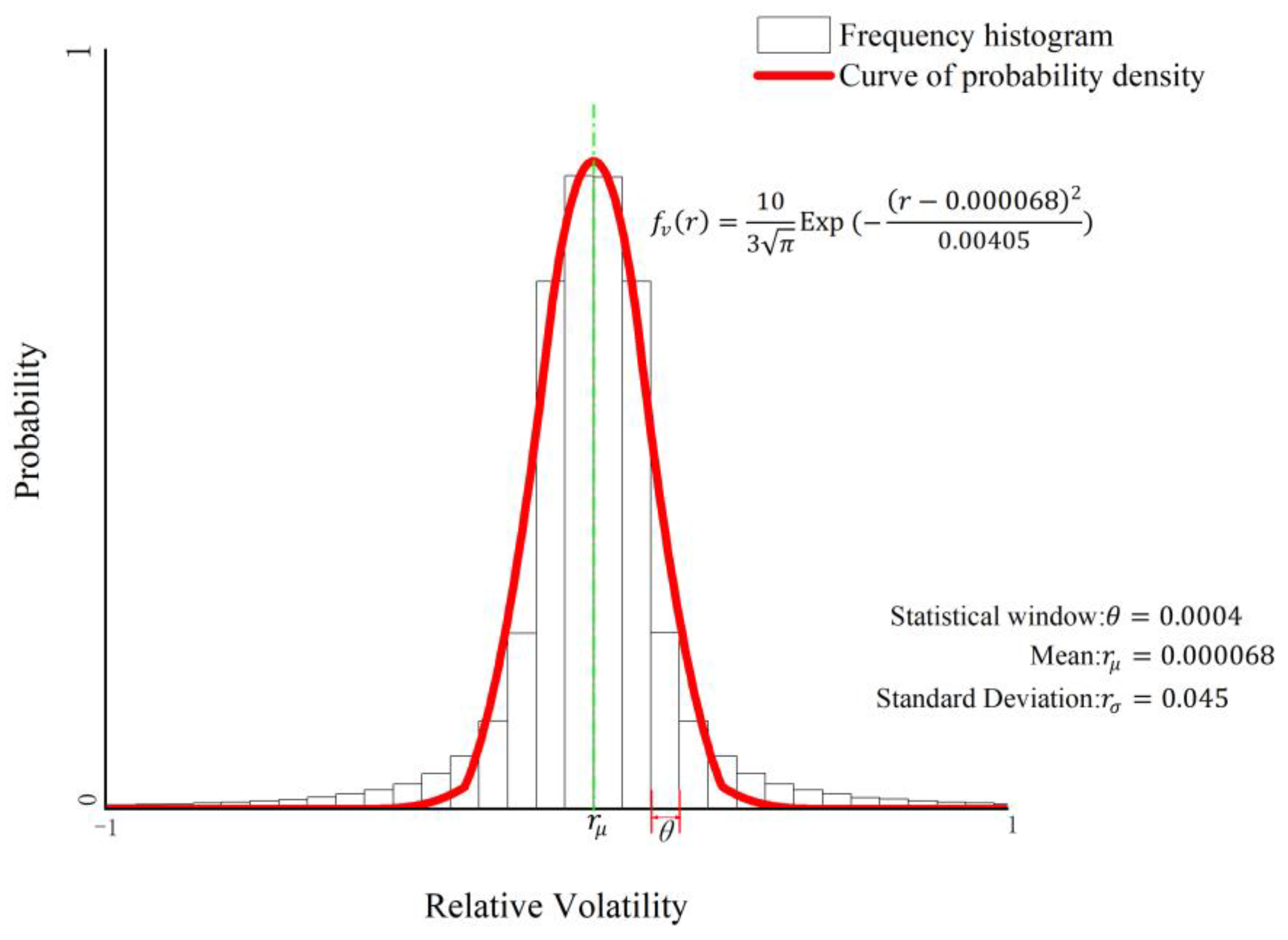
In this paper, the probability vector r v - P V is obtained by statistically calculating the relative fluctuation of wind speed at wind farms throughout the year, which is approximately the commonly used normal distribution, with a mean of the relative volatility of 0.000068, a standard deviation of 0.045, and a statistical wide-window factor of 0.00043478. The probability-vector distribution is shown in Figure 2.
In Figure 2, the interval (−1, 0) indicates the frequency of downward volatility in wind speed, and the interval (0, 1) indicates the frequency of wind speed in the upward volatility. The difference from the statistical distribution of wind speed [1] is the statistical distribution of wind speed is a statistic of instantaneous values, whereas relative volatility is the change in the wind speed value relative to the previous state; f v r μ shows that the main trend of the time series period fluctuating in the vicinity of the wind speed r μ plays a decisive role in the accumulation of quantitative changes. In addition, the r μ is the probability corresponding to the apex.
Generally, the probability vector r x - P V length is assumed to be N. To describe the volatility of the ratio change, the correlation qualities of the center and shift of the ratio fluctuation are given below.
Nature 1. (Center Vector and Vector Center): 
There is always a maximum probability  P m a x n  on  r x - P V  which is the center vector, and its corresponding vector is subscripted as the center of that vector which is indicated by C, C = n (The main cause of the change in status plays a decisive role).
Nature 2. (Vector Offset): 
On  r x - P V , if  p n > 0 The distance between  p n  and the maximum probability  P m a x c  is called the vector offset and is denoted by  l n , where  l n = n C .   C  is a special case of vector offset when  l n = 0  (accumulation of quantitative change states).
The relative position of the vector center C   a n d   N 2 noted by L :
L = C N 2
W = W _ r W _ l + 1
In Equation (5), when L > 0 , the main trend is in an upward state. When L < 0 , the main trend is in a downward state with a fluctuation range of [ 2 C 1 N 1 , 2 C + 1 N 1 ). When L = 0 , the main trend is in a plateau state with a ratio interval of [ 1 N , 1 N ). Each fluctuation offset l n on r x - P V is associated with the center C with the same fluctuation range [ 2 n 1 N 1 , 2 n + 1 N 1 ).
The above r x - P V is a statistical composition of the ratio assuming that θ is known. In fact, a different θ means different intervals of statistical domain values with different construction r x - P V . In order to minimize the error and not affect the subsequent prediction results, it is necessary to find the optimal θ value.
θ Value optimization: N telescopic method
According to the law of large numbers and the central limit theorem, in a normal state, parameter changes are in line with a normal distribution. The basic idea of finding the optimal θ value is: For a θ given initial θ 0 and relative volatility data set R , determine its initial vector size N . Construct the current θ corresponding r x - P V , and fit the normal distribution function of r x - P V . Construct a new vector of the same size by fitting the normal distribution function, then generate r x - P V . Calculate the Euclidean distance d i s t of and r x - P V , and record the current θ , d i s t value. Repeat the previous process by scaling to change N . Update the θ value until the end of the cycle with the smallest d i s t value. Then, the θ value of minimum d i s t is output. The objective of finding the optimum is achieved with the following objective function:
m i n d i s t r x _ P V , r x _ P V = i = 1 M a t h . f l o o r 2 θ p i p i 2
In Equation (7): p i   is the probability   o n r x - P V , p i   is the probability on   r x _ P V .

2.3. r x _ P V Volatility Assessment Indicators

In the stable state of the parameter variable, the ratio frequency statistics of the wind turbine SCADA data conform to the normal distribution characteristics and are relatively easy to identify, however, when it is in an abnormal operating state or there is a potential risk of parameter fluctuations, the implied state value can be evaluated by the distribution characteristics of the ratio vector n _ P V (that is with fluctuation offset), and the P V fluctuation influence factor and fluctuation-evaluation function are introduced below. The n _ P V vector is P t = p t , 1 , p t , 2 , , p t , C , , p t , N , N is the vector size, and its fluctuation influence factor is:
δ r i = 1 2 π σ 1 e r i r C 2 2 σ 2
Among them, according to the normal distribution on C t 2.58 σ , C t + 2.58 σ , the area of the horizontal axis interval is 99.730020%, which is within the error control range, so σ L θ 10.16 ( L N ) . Each vector of P V corresponds to a fluctuation influence factor δ r i . It can be seen from Equation (6) that under the same probability conditions, when the fluctuation factor is zero, the greater the offset with the distance, the greater the impact on the state change. When the offset reaches or exceeds 2.58 σ , its effect approaches 1 infinitely, therefore, the fluctuation influence factor takes a range of values δ [ 0,1 ) .
The r x _ P V volatility assessment indicators:
Γ t r x _ P V = i = 1 N p t , i M a t h . a b s ( i C t ) N 2 + δ r i 2
From Equations (8) and (9), it can be seen that r x - P V . Wave is the sum of the evaluations of each offset vector. Each offset vector consists of the value squared by the sum who’s each degree of offset M a t h . a b s ( i C t ) N and volatility factor δ r i multiplied the probability p t , i of the vector. On the ratio vector, any range of ratio domain values implies different fluctuation values and the larger Γ p v , t , the greater the fluctuation and the greater the risk. The risk implied by the volatility domain value interval [ 2 C 1 N 1 , 2 C + 1 N 1 ) of the central vector p C is composed of two parts: the p C risk Γ c within the interval and the 1 p C risk r c ~ outside the interval. In general, it is considered Γ c = 0 , as there is zero risk, and the risk outside the interval is divided equally into each of the other intervals. Therefore, Γ c ~ = Γ t P t , C t . Vector offset is the risk relative to the center vector Γ n Γ c ~ , calculated using the offset and probability values.

3. Wind Velocity and Feature Analysis

3.1. Feature Analysis of r v

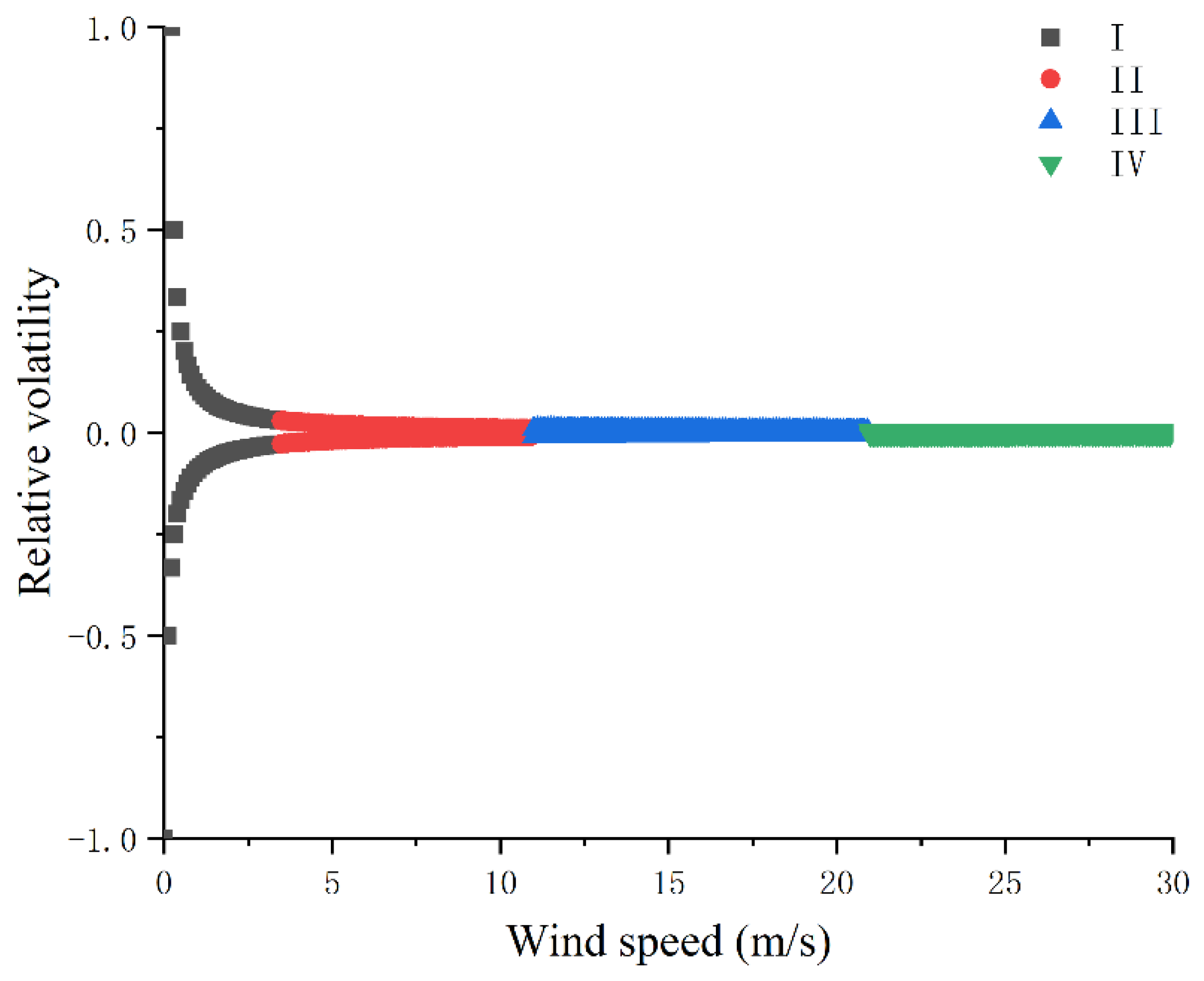
Assuming an average variation in wind speed, the curve of the relative wave rate of wind speed in each operating zone of the turbine is plotted against the average speed of the wind under ideal conditions according to the definition of relative volatility rate as follows:
The four different zones are represented by I, II, III, and IV. Zone I : when v   < v c u t i n , p = 0 , representing the pending area. Zone I I : when v c u t i n < v   <   v r , p reaches its maximum wind energy capture power, reflecting the maximum wind energy tracking zone. Zone I I I : when v r < v   <   v c u t o u t , p = p r , indicating the constant power zone. Zone I V : when v > v c u t o u t , wind turbine braking shutdown, p = 0 , it is in the no-output power feedback control state, signifying the shutdown protection zone.
As can be seen from Figure 3, under the premise of the average speed change ( v = a , a is a constant ) , the relative volatility gradually becomes smaller as the wind speed gradually increases, while in the I zone, the relative volatility varies more, and in the II, III, IV regions, the relative volatility varies less, and when a approaches zero, r v tends to zero:
r v = lim a 0 ( v k v k 1 1 ) = 0
The upper and lower bounds of the relative volatility of wind speed r v in each operating area are discussed below.
Zone I ( 0 v < v c u t i n ), when v t 1 v c u t i n , v t 0 , at this time, the lower bound of r t is 1 , since v t 1 0 , no upper bounds, r v 1 .
Zone II ( v c u t i n v < v r ), when v t v r , v t 1 v c u t i n , the upper bound r v : v r v c u t i n 1 ; when v t v c u t i n , v t 1 v r , r v is the lower bound: v c u t i n v r 1 , that is v c u t i n v r 1 < r v < v r v c u t i n 1 .
Zone III ( v r v < v c u t o u t ). The same goes for it: v r v c u t o u t 1 < r v < v c u t o u t v r 1 .
Zone VI ( v c u t o u t v ). The same goes for it: r v > 1 .
Combined with the above:
r v 1      0 v < v c u t i n v c u t i n v r 1 < r v < v r v c u t i n 1    v c u t i n v < v r v r v c u t o u t 1 < r v < v c u t o u t v r 1 v r v < v c u t o u t r v > 1        v c u t o u t v
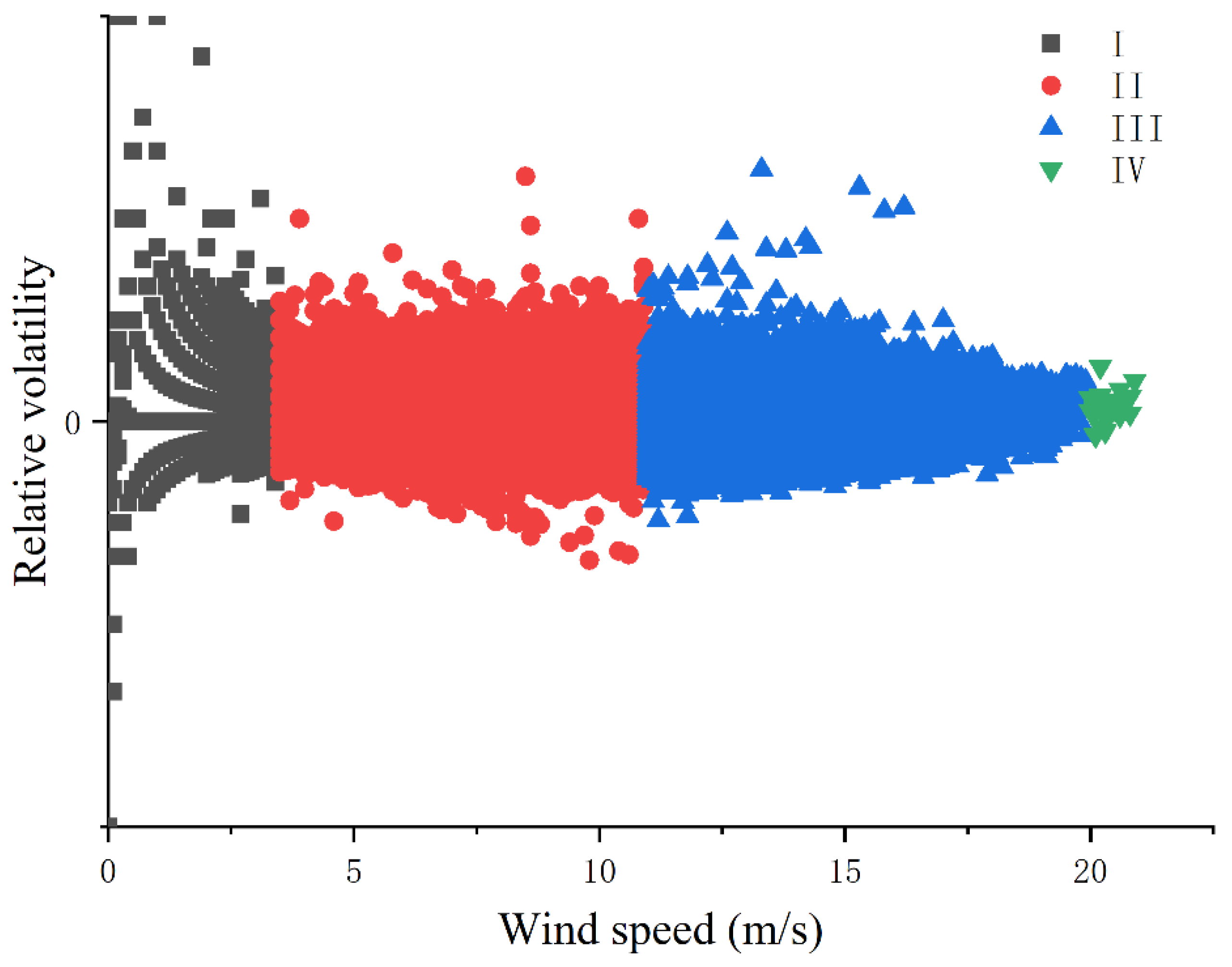
The statistics of the wind speed relative volatility data for 2 MW wind turbines in this model show that with the rise of wind speed, its r v change range tends to be smaller, and the relative volatility data in the IV operation area is less, and the relative volatility of wind speed throughout the year is relatively stable, with the value of zone I: r v is between −0.5 and 0.75, the value of zone II and III: r v is between −0.25 and 0.25, and the relative volatility of zone IV is close to zero. The statistical results are basically consistent with those shown in Figure 2 above, and also meet the theoretical value range of the relative volatility of wind speed in Equation (11), as shown in Figure 4.
The previous analysis is the analysis of the range of relative fluctuation in wind speed across four working areas. Combined with the law of nature, the change in wind speed is cyclical, and the difference in the relative volatility change of each quarter and month is analyzed. Statistics show that the mean relative fluctuations and standard deviations vary from month to month and the results are shown in Table 1.
As can be seen from Table 1, the relative volatility of the wind speed at the wind farm from July to October is low, all below 0.025, while the fluctuation in the wind speed from November and December to June is relatively high, with January being the highest, indicating that the variation in wind speed is most pronounced in January. Over the 12 months, the mean relative volatility changed from 0.023236–0.028769, and the standard deviation of relative volatility changed from 0.033648–0.041289.
Then, according to the normal distribution with an interval area of 99.730020% on the horizontal axis of μ 2.58 σ , μ + 2.58 σ , the confidence interval can be calculated for each operating area and for different months, as shown in Table 2.
In Table 2, the relative volatility of wind speed is 99.730020% under the condition of confidence level, and the confidence width and narrowness of each wind-speed power zone and each month range between 0.000358–0.020732, generally was narrow. Specifically, Zone I has a relatively high annual confidence width and narrowness, with each month above 0.012500; Zones II and III have relatively stable annual confidence width and narrowness, both fluctuating around 0.01. Meanwhile, the annual confidence width and narrowness of Zone IV exhibit significant changes, with the highest in August (0.020732) and the lowest in December (0.000358). The statistical description of this table shows that the sample size of wind speed in Zone I is relatively small throughout the year; The sample size in Zones II and III is large; the distribution of high wind-speed samples in Zone IV is uneven by month, with fewer samples in August and more in December, and the variation of high wind speed in Zone IV fluctuated greatly.

3.2. Feature Analysis of r v _ P V

This section performs feature analysis on r v _ P V , where the monthly time series is used as the data period and the optimal statistical-window parameter value is θ = 0.043478 (That is, r v _ P V length N = 46). For each month of the year, there are 12 structures r v _ P V for the relative volatility of onsite SCADA wind speed. The corresponding fluctuation-evaluation indicators, attribute characteristics, distribution characteristics, and other characteristic values are counted and presented in Table 3.
In the 12 months of the year, the fluctuation centers of 12 r v _ P V are 23, and the expected value of the fitted distribution is −0.02, and the standard deviation ranges 0.008544–0.023314. The range of the fluctuation-evaluation index values is between 1.802787 and 6.025606. The fluctuation-evaluation index values of the 3rd, 4th, 7th, 9th, 10th and other 5 months are about 1.8, with a small fluctuation interval (= W _ r W _ f + 1), and a small characteristic value of the standard deviation of the fitted normal distribution, indicating a relatively concentrated relative volatility of wind speed. The fluctuation-evaluation index values in the 2nd, 5th, 6th, and 12th months all exceeded 5.0, indicating that the relative volatility distribution of wind speed is dispersed, and its fluctuation range was large, indicating a significant change in wind-speed range. At the same time, it can be seen that the trend of the characteristic value of the fluctuation-evaluation index has a certain correlation with the standard deviation σ (or coefficient of variation σ μ ) of the r v _ P V distribution.
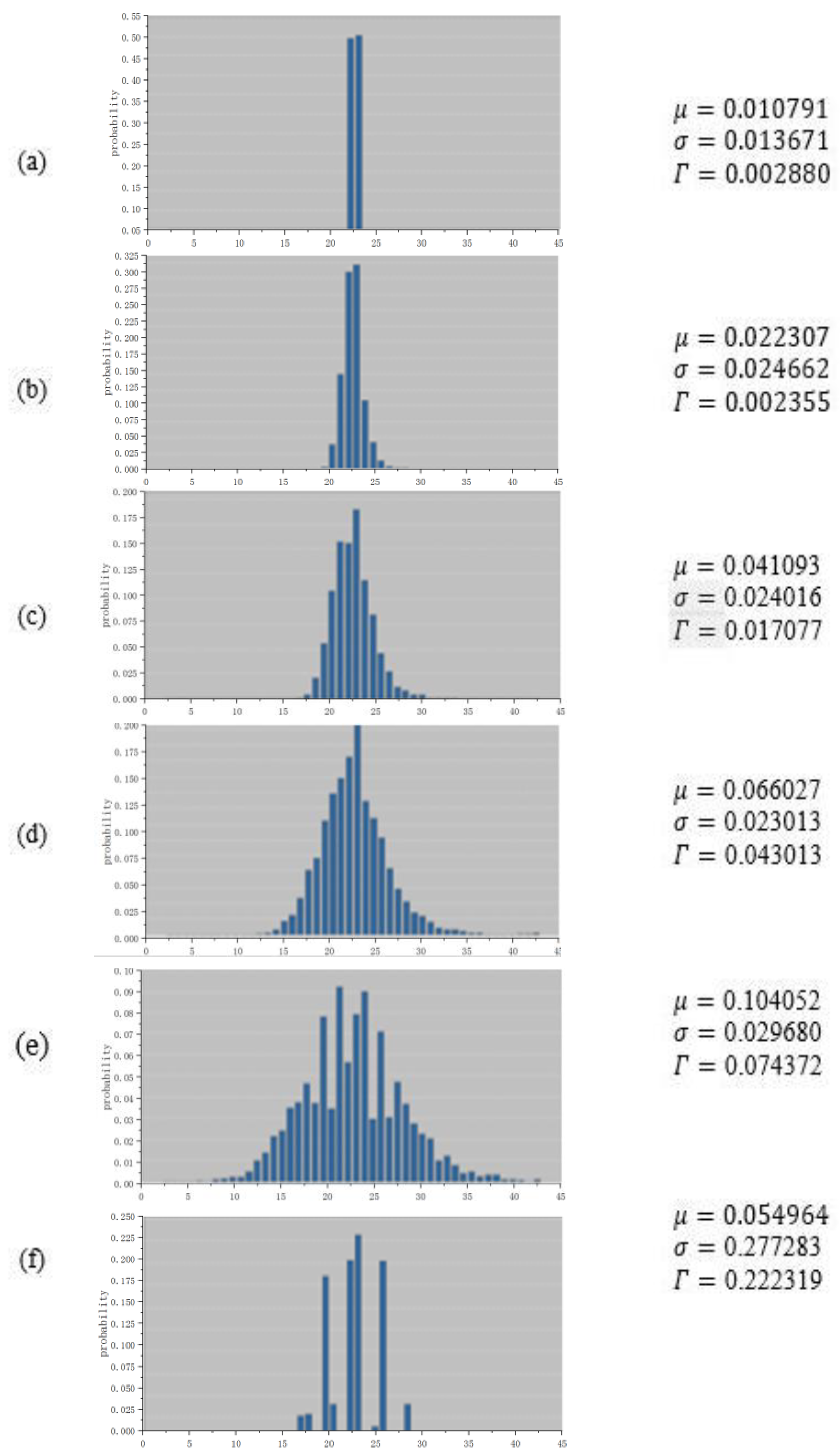
The previous is based on each month as the time-series period, and the following is the r v _ P V distribution model of six typical states with a period of 1 h.
In Figure 5, class (a) r v _ P V : the bars representing the relative volatility probability are sparse and concentrated, typically 1–2. The fluctuation interval is small ( W = 2 ) and the peak value is prominent ( f μ = 0.503611 , σ = 0.013671 ). The wind speed remains relatively constant or changes minimally at a steady pace. Class (b) r v _ P V : there are more than three bars that represent the relative volatility probability, the fluctuation interval is small ( W = 10 ), the distribution is more concentrated, the peak value is obvious ( f μ = 0.321667 , σ = 0.024662 ), and changes in wind speed can be observed. Class (c) r v _ P V : the distribution of bars representing the relative volatility probability has a flat trend, with a small fluctuation interval ( W = 19 ) and a distinct peak ( f μ = 0.18972 , σ = 0.024016 ), and a significant change in wind speed can be observed. Class (d) r v _ P V : the distribution shape of the bar box representing the relative volatility probability is flat and the fluctuation range exceeds half of the horizontal axis ( W = 30 ). There is a peak ( f μ = 0.133056 , σ = 0.023013 ) and the wind speed changes greatly. Class (e) r v _ P V : the distribution representing the relative volatility has multiple peaks, the volatility interval value is larger ( W = 38 ), the value of the volatility assessment index increases, and the difference between the probability distribution and the normal distribution is obvious. Class (f) r v _ P V : the distribution representing relative volatility has multiple peaks, the volatility interval value is large, and there is no obvious feature of normal distribution.

4. Correlation Analysis of Wind Velocity r v and Wind Turbines Power Output r p

4.1. The v-p Relative Volatility Correlation Analysis

According to Equation (2), the relative fluctuation of the output power is calculated as follows:
r p , k = p k p k 1 p k 1 p k 1 0
Substitute Equation (1) into the above equation:
r p , t = C p k C p k 1 × ( v k v k 1 ) 3 1
Among them, according to Equation (2):
C p k C p k 1 = r C p , k + 1
v k v k 1 = r v , k + 1
Substituting Equations (14) and (15) into Equation (13) yields:
r p , k = r C p , k + 1 r v , k + 1 3 1
Equation (16) represents the general relationship between power and wind speed, as well as the relative volatility of the wind-energy utilization coefficient, denoted by r C p , k and r v , k , respectively. It is evident that there is relative volatility of wind speed. It can be seen that the relative volatility r p , k of the output power is a high-order function of the relative volatility of the wind-energy utilization coefficient r C p , k and the relative volatility of wind speed r v , k . In the effective working area of wind-turbine operation, the output power is controlled by controlling the wind speed and wind-energy utilization coefficient, and the relationship between output power, wind speed, and wind-energy utilization coefficient is discussed in the effective working area (Zone II and Zone III) below.
In Zone II, that is v c u t i n v < v r , C p , is the maximum wind energy utilization coefficient and a fixed value, v , is variable.
Equation (1) is available for derivation:
d p = 3 2 ρ A C p v 2 d v
Use Equation (1) to divide both sides by the above formula:
d p p = 3 d v v
Substituting Equation (3) into Equation (18) yields:
r p , k p k 1 p k d t = 3 × r v , k v k 1 v k d t
Simplify the above formula:
r p , k = 3 r v , k 1 2 r v , k
In Zone III, when v r v < v c u t _ o u t , p is rated output power and v   a n d   C p are variable.
Equation (1) is for total derivation:
d p = 1 2 ρ A v 3 d C p + 3 2 ρ A C p v 2 d v
Since d p = 0 :
1 2 ρ A v 3 d C p = 3 2 ρ A C p v 2 d v
Transforms are available:
d C p C p = 3 d v v
Similarly, substitute Equation (3) into Equation (23):
r C p , k C p k 1 C p k d t = 3 × r v , k v k 1 v k d t
Simplify the above equation:
r C p , k = 3 r v , k 4 r v , k + 1

4.2. Relationship Curve of r v and r p , r C p

Combined with the operational principle of wind turbines, this section emphasizes the correlation between the relative fluctuations of wind speed and output power in Zones II and III of wind-turbine operation.
In Zone II, the wind turbine’s maximum power output coincides with the maximum wind-energy tracking zone. The relative volatility curve of output power generated by wind turbines under different relative fluctuations of wind speeds is represented by v - p relative volatility, as shown in Figure 6.
In this zone, the maximum wind-energy utilization coefficient C p is the maximum, and the output power is a nonlinear third-order function of wind speed, and after converting to the relative volatility of parameters, the relative volatility of output power is related to the relative volatility of wind speed.
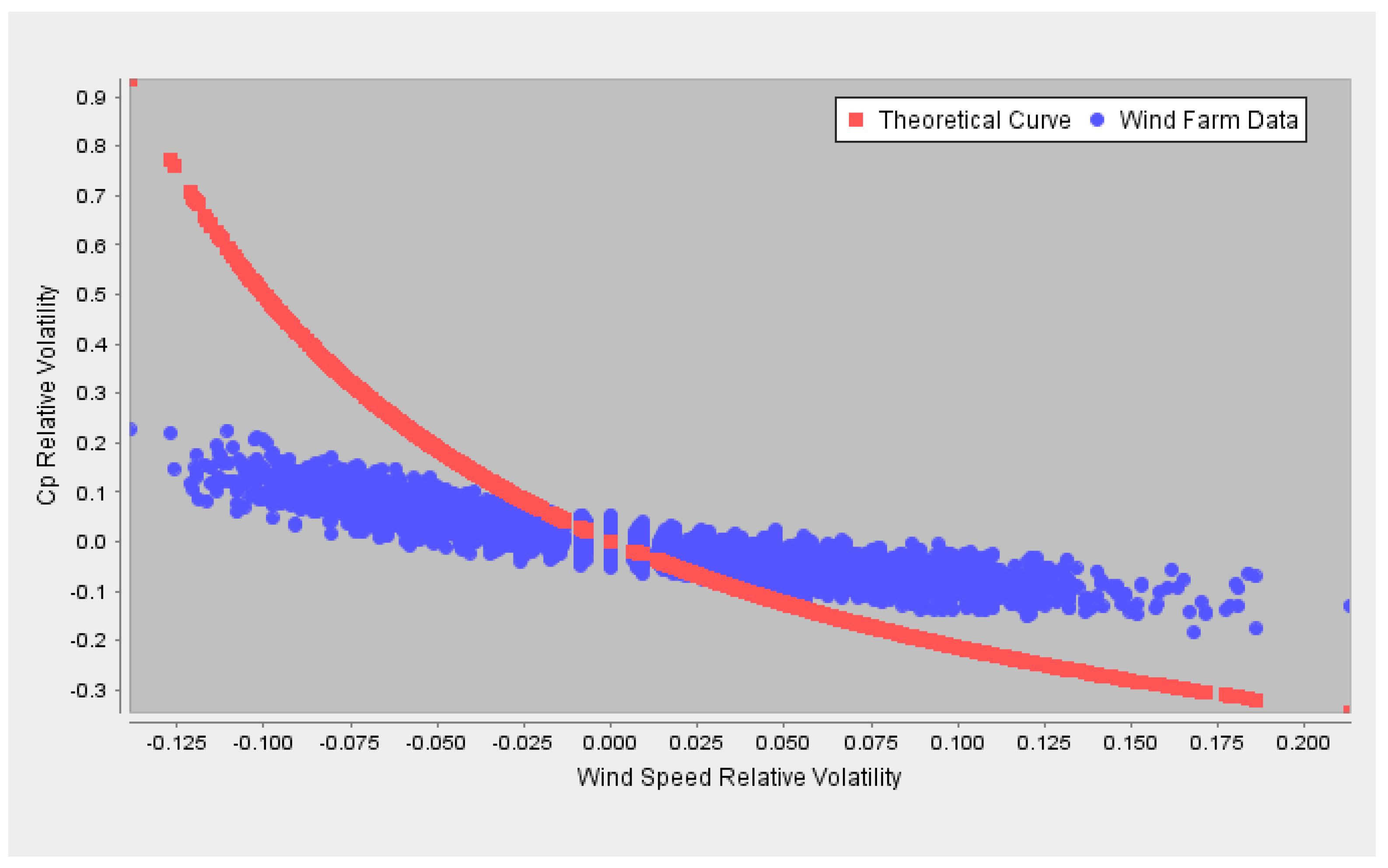
In Zone III, Figure 7 compares and analyzes the change range and trend of the relative volatility of wind-speed relative volatility and wind-energy utilization coefficient of ideal volatility and onsite statistical value. It can be observed that the relationship of r v and r C p is inversely proportional for r v [ 0.25,025 ] . As r v increase, r C p continues to decrease. In the range where r v is close to zero, the ideal value of r C p and the statistical value are nearly the same. However, with the increase of the r v absolute value, the difference between the two values increases significantly. Nonetheless, the overall trend remains consistent.

5. Discussion

The purpose of this study is to extract the wind-speed variation pattern from onsite SCADA data, analyze the correlation between relative volatility of wind speed and power, establish a wind-power volatility curve model, and provide a basis for evaluating the performance of wind turbines. The novelty and advantages of the method in this paper are that by converting the wind speed and power in SCADA data into dimensionless relative volatility, the non-normal distribution of wind speed is converted into an approximate normal distribution of the relative volatility of wind speed to facilitate the extraction of distribution characteristics. By introducing relative volatility, a linear relationship between the derivatives of wind speed, power, and wind-energy utilization coefficient was discovered.
Relative volatility is a dimensionless variable that represents the change in SCADA data parameters. Future research can explore the following directions:
  • Improvements in modeling methods based on relative fluctuation rate: current wind power curve modeling methods are mostly based on statistical methods, however, these methods have limited modeling capabilities for complex wind fields and working environments. Future research can explore new methods based on machine learning, deep learning, and other methods for the wind power relative fluctuation rate curve modeling, to improve modeling accuracy and applicability;
  • Consideration of related factors: the magnitude and distribution characteristics of the relative fluctuation rate are related to multiple factors, such as wind field environment, turbine type, and turbine operation status. Future research can explore how to consider the impact of these factors on the relative fluctuation rate and incorporate them into modeling to improve the accuracy of wind-power curve modeling;
  • Indepth application research: in addition to wind-power curve modeling itself, the relative fluctuation rate can also play an important role in power forecasting for wind farms, turbine health monitoring, and other applications. This work can help in the prevention of a possible blackout due to the mismatch between the production and the consumption. Future research can explore how to apply the relative fluctuation rate to more practical application scenarios to improve the economic and reliable performance of wind farms.

6. Conclusions

This paper investigated the fluctuation patterns of onsite wind-speed and wind-turbine power-output parameters using SCADA data from a wind farm, which provides valuable insights for SCADA data mining. The main findings of this study are presented below.
  • Utilizing SCADA data and wind turbine runtime sequence rules, this study defined the relative volatility r x and its probability model r x - P V , to quantify the degree and trend of the data and converted the physical meaning parameters’ degree of change and trend into dimensionless relative volatility. Unlike the partial normal distribution of traditional wind speed, r x - P V exhibited obvious normal distribution characteristics, and its feature values could be extracted by fitting the normal distribution function. Additionally, the defined r x - P V volatility evaluation index can evaluate the relative volatility distribution characteristics of parameters in a certain time-series period, which provided a theoretical basis for an indepth analysis of the change law of wind speed and the wind-speed model;
  • The statistical analysis of wind speed’s relative volatility distribution characteristics revealed significant variations in the relative volatility of different wind speed operating areas in a year. Based on the SCADA data of the wind farm, the relative volatility of Zone I fell between −0.5 and 0.75, while for Zone II and III, it ranged between −0.25 and 0.25. Zone IV exhibited fewer high wind-speed data, and its relative volatility was close to zero. The relative volatility distribution performance of different months of the year also differed: three, four, seven, nine. The relative volatility of the wind speed in 10 and 5 months was relatively concentrated, and the wind-speed change was relatively stable; The relative volatility distribution of wind speed in the 2nd, 5th, 6th, and 12th months was scattered, and the fluctuation range was large, indicating that the wind-speed change range was large. Additionally, through the six typical-distribution statistics of the small period (1 h), it was found that the wind-speed fluctuation-evaluation index and the distribution standard deviation show obvious positive proportional relationship. This means that the larger the standard deviation, the larger the eigenvalues of the evaluation index, and the more dispersed the relative volatility distribution of wind speed. Conversely, the smaller the eigenvalues of the evaluation index, the more concentrated the relative volatility distribution of wind speed;
  • The relative fluctuation of the correlation between wind speed and power output was analyzed, and the relationship between wind speed and power output was derived mathematically. There was a relationship d p p = 3 d v v in Zone II. There was a relationship d C p C p = 3 d v v in Zone III, and the relative volatility of power and the relative volatility of the wind energy utilization coefficient could be expressed as a function of the relative volatility of the wind speed. By counting the relative volatility of the wind speed and output-power data of the onsite SCADA and calculating the fluctuation-evaluation index values respectively, it was found that the two had similar change trends;
  • The magnitude and distribution characteristics of the relative fluctuation rate were related to multiple factors, such as wind field environment, turbine type, and turbine operation status. The influence of the above factors was not considered in this article. Future research can explore how to consider the impact of these factors on the relative fluctuation rate and incorporate them into modeling to improve the accuracy of wind-power curve modeling.

Author Contributions

Conceptualization, writing—review & editing: S.Q. Data Curation, methodology: D.L. All authors have read and agreed to the published version of the manuscript.

Funding

The authors disclosed receipt of the following financial support for the research, authorship, and publication of this article: The work described in this paper is funded by the Natural Science Foundation of China (Grant No. 51475160), the Natural Science Foundation of Hunan Province of China (Grant No. 2018JJ5010).

Institutional Review Board Statement

The study did not involve humans and animals. The study did not require ethical approval.

Informed Consent Statement

The study did not involve humans.

Data Availability Statement

You can contact the author via email to obtain data that supports the report results.

Conflicts of Interest

The authors declare that there is no potential conflict of interest with respect to the research, authorship, and/or publication of this article.

Abbreviations

The abbreviation list in this article.
Symbol NameDescription
p Output power
ρ Air density
A Wind turbine blade sweep area
C p Wind energy utilization coefficient, it is a function of pitch angle and blade tip speed ratio
v c u t i n Cut into the wind speed
v r Rated wind speed
v c u t o u t Cut out the wind speed
p r Rated output power
{ x ( t ) } Data series of SCADA parameter
k Time series, k [ 0,1 , 2,3 , 4 , , k , ]
r x , k Relative volatility, x refers to parameters in general, k refers the kth moment
r x _ P V Probability vector of Relative volatility
r v , k Relative volatility of wind speed
r p , k The relative volatility of the output power
N Vector length of r x - P V
θ Statistical window width factor for constructing r x - P V
C Vector center of r x - P V
L Vector offset of r x - P V
W Fluctuating width of r x - P V
W _ l Fluctuation left border of r x - P V
W _ r Fluctuation right border r x - P V
Γ Volatility assessment indicators of r x - P V

References

  1. Hossain, J.; Mahmud, A. Large Scale Renewable Power Generation: Advances in Technologies for Generation, Transmission and Storage; Springer: Berlin/Heidelberg, Germany, 2014. [Google Scholar]
  2. Hosseini, S.H.; Tang, C.Y.; Jiang, J.N. Calibration of a Wind Farm Wind Speed Model with Incomplete Wind Data. IEEE Trans. Sustain. Energy 2014, 5, 343–350. [Google Scholar] [CrossRef]
  3. Carta, J.A.; Ramirez, P.; Velazquez, S. A review of wind speed probability distributions used in wind energy analysis: Case studies in the Canary Islands. Renew. Sustain. Energy Rev. 2009, 13, 933–955. [Google Scholar] [CrossRef]
  4. Khamees, A.K.; Abdelaziz, A.Y.; Ali, Z.M.; Alharthi, M.M.; Ghoneim, S.S.; Eskaros, M.R.; Attia, M.A. Mixture probability distribution functions using novel metaheuristic method in wind speed modeling. Ain Shams Eng. J. 2022, 13, 101613. [Google Scholar] [CrossRef]
  5. Sumair, M.; Aized, T.; Bhutta, M.M.A.; Siddiqui, F.A.; Tehreem, L.; Chaudhry, A. Method of Four Moments Mixture-A new approach for parametric estimation of Weibull Probability Distribution for wind potential estimation applications. Renew. Energy 2022, 191, 291–304. [Google Scholar] [CrossRef]
  6. Chen, H.; Anfinsen, S.N.; Birkelund, Y.; Yuan, F. Probability distributions for wind speed volatility characteristics: A case study of Northern Norway. Energy Rep. 2021, 7, 248–255. [Google Scholar] [CrossRef]
  7. Song, D.; Yan, J.; Zeng, H.; Deng, X.; Yang, J.; Qu, X.; Rizk-Allah, R.M.; Snášel, V.; Joo, Y.H. Topological Optimization of an Offshore-Wind-Farm Power Collection System Based on a Hybrid Optimization Methodology. J. Mar. Sci. Eng. 2023, 11, 279. [Google Scholar] [CrossRef]
  8. Colombo, L.; Corradini, M.L.; Ippoliti, G.; Orlando, G. Pitch angle control of a wind turbine operating above the rated wind speed: A sliding mode control approach. ISA Trans. 2020, 96, 95–102. [Google Scholar] [CrossRef] [PubMed]
  9. Oliveira, T.D.; Tofaneli, L.A.; Santos, A.L.B. Combined effects of pitch angle, rotational speed and site wind distribution in small HAWT performance. J. Braz. Soc. Mech. Sci. Eng. 2020, 42, 425. [Google Scholar] [CrossRef]
  10. Song, D.; Li, Z.; Deng, X.; Dong, M.; Huang, L.; Yang, J.; Su, M.; Joo, Y. Deep optimization of model predictive control performance for wind turbine yaw system based on intelligent fuzzy deduction. Expert Syst. Appl. 2023, 221, 119705. [Google Scholar] [CrossRef]
  11. Morshedizadeh, M.; Rodgers, M.; Doucette, A.; Schlanbusch, P. A Case Study of Wind Turbine Rotor Over-Speed Fault Diagnosis Using Combination of SCADA Data, Vibration Analyses and Field Inspection. Eng. Fail. Anal. 2023, 146, 107056. [Google Scholar] [CrossRef]
  12. Morrison, R.; Liu, X.; Lin, Z. Anomaly detection in wind turbine SCADA data for power curve cleaning. Renew. Energy 2022, 184, 473–486. [Google Scholar] [CrossRef]
  13. Liu, D.; Zhang, F.; Dai, J.; Xiao, X.; Wen, Z. Study of the pitch behaviour of large-scale wind turbines based on statistic evaluation. IET Renew. Power Gener. 2021, 15, 2315–2324. [Google Scholar] [CrossRef]
  14. Xing, Y.; Gu, Y.J.; Ma, L. Wind Turbine Status Assessment Considering Wind Speed Fluctuations. Process Autom. Instrum. 2019, 40, 28–32. [Google Scholar] [CrossRef]
  15. Zhang, F.; Liu, D.S.; Dai, J.C.; Wang, C.; Shen, X.B. An operating condition recognition method of wind turbine based on SCADA parameter relations. Jixie Gongcheng Xuebao/J. Mech. Eng. 2019, 55, 1–9. [Google Scholar] [CrossRef]
  16. Cheng, S.Y.; Liu, H.; Zeng, T.S.; Chen, H.S.; Wang, Z.; Zhu, X.N. Component importance analysis of wind turbine based on SCADA parameter relations. Renew. Energy Resour. 2021, 39, 1335–1341. [Google Scholar]
  17. Wang, Y.; Hu, Q.; Srinivasan, D.; Wang, Z. Wind Power Curve Modeling and Wind Power Forecasting with Inconsistent Data. IEEE Trans. Sustain. Energy 2018, 10, 16–25. [Google Scholar] [CrossRef]
  18. Nasery, P.; Ezzat, A.A. Yaw-adjusted wind power curve modeling: A local regression approach. Renew. Energy 2023, 202, 1368–1376. [Google Scholar] [CrossRef]
  19. Zha, W.; Jin, Y.; Sun, Y.; Li, Y. A wind speed vector-wind power curve modeling method based on data denoising algorithm and the improved Transformer. Electr. Power Syst. Res. 2023, 214, 108838. [Google Scholar] [CrossRef]
  20. Wang, Y.; Duan, X.; Zou, R.; Zhang, F.; Li, Y.; Hu, Q. A novel data-driven deep learning approach for wind turbine power curve modeling. Energy 2023, 270, 126908. [Google Scholar] [CrossRef]
  21. Soliman, M.S.; Belkhier, Y.; Ullah, N.; Achour, A.; Alharbi, Y.M.; Al Alahmadi, A.A.; Abeida, H.; Khraisat, Y.S.H. Supervisory energy management of a hybrid battery/PV/tidal/wind sources integrated in DC-microgrid energy storage system. Energy Rep. 2021, 7, 7728–7740. [Google Scholar] [CrossRef]
  22. Al Alahmadi, A.A.; Belkhier, Y.; Ullah, N.; Abeida, H.; Soliman, M.S.; Khraisat YS, H.; Alharbi, Y.M. Hybrid wind/PV/battery energy management-based intelligent non-integer control for smart DC-microgrid of smart university. IEEE Access 2021, 9, 98948–98961. [Google Scholar] [CrossRef]
  23. Fotis, G.; Vita, V.; Maris, T. Risks in the European Transmission System and a Novel Restoration Strategy for a Power System after a Major Blackout. Appl. Sci. 2023, 13, 83. [Google Scholar] [CrossRef]
  24. Vita, V.; Fotis, G.; Pavlatos, C.; Mladenov, V. A New Restoration Strategy in Microgrids after a Blackout with Priority in Critical Loads. Sustainability 2023, 15, 1974. [Google Scholar] [CrossRef]
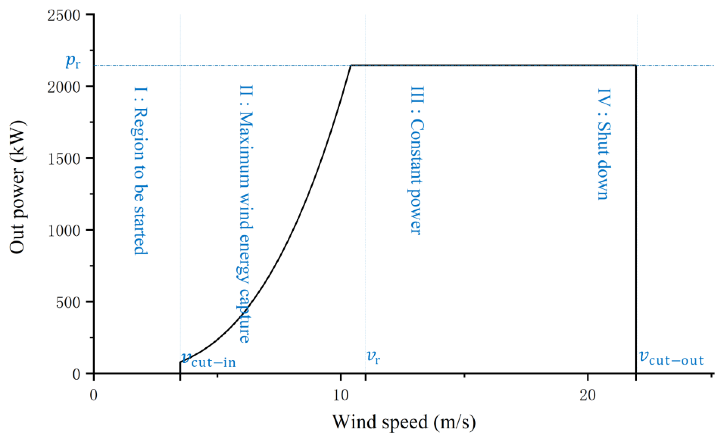
Figure 1. Operation status of the wind turbine.
Jmse 11 00967 g001
Figure 2. Probability distribution of the wind speed relative volatility.
Jmse 11 00967 g002
Figure 3. Scatter Chart about the relative volatility of wind speed that changes at a constant speed.
Jmse 11 00967 g003
Figure 4. Scatter Chart of r v from SCADA data.
Jmse 11 00967 g004
Figure 5. Six typical r v _ P V .
Jmse 11 00967 g005
Figure 6. Output power relative volatility curve.
Jmse 11 00967 g006
Figure 7. C p relative volatility curve in Zone III.
Jmse 11 00967 g007
Table 1. Statistics on relative volatility of wind speed over 12 months.
Relative Volatility of Wind SpeedMonth
ItemArea123456789101112
MeanI−0.001550−0.001710−0.001852−0.001577−0.001418−0.001909−0.001786−0.001681−0.000944−0.001361−0.001652−0.001678
II−0.0002610.0000910.0004220.0003310.0001920.0003690.0008070.0007310.0009050.0007820.0005360.000487
III0.0058620.0048850.0067280.0043370.0034260.0053640.0065760.0057090.0064070.0063860.0046830.005331
IV0.0370680.0194730.0138320.0103620.0120360.0126220.0116140.0135100.0106210.0257970.0147510.006319
Whole0.0003950.000179−0.0000840.0002490.0004710.000016−0.000336−0.0004440.000116−0.0000160.0002330.000190
Standard
Deviation
I0.0514770.0568400.0572750.0593650.0604110.0606750.0560410.0557700.0492860.0522400.0526060.052234
II0.0398370.0382280.0378680.0379820.0429490.0355210.0340710.0343550.0340620.0359070.0393740.038026
III0.0475080.0427030.0431230.0450440.0437790.0419400.0398070.0445060.0435960.0413530.0466600.041932
IV0.0331300.0382830.0377500.0497810.0457690.0398870.0434110.0633870.0488290.0317120.0465250.008325
Whole0.0442670.0449570.0465980.0457290.0473200.0452690.0459500.0473750.0417800.0435700.0445600.043274
Table 2. The 12-month confidence interval for wind speed relative volatility.
Month of YearConfidence Interval of Relative Volatility of Wind Speed
IIIIIIIV
1(−0.008388, 0.005286)(−0.004356, 0.003833)(0.000039, 0.011686)(0.034236, 0.039900)
2(−0.010046, 0.006625)(−0.003679, 0.003862)(0.000180, 0.009590)(0.015692, 0.023254)
3(−0.010316, 0.006612)(−0.003278, 0.004122)(0.001931, 0.011527)(0.010155, 0.017509)
4(−0.010671, 0.007515)(−0.003391, 0.004053)(−0.000898, 0.009572)(0.003968, 0.016756)
5(−0.010834, 0.007998)(−0.004566, 0.004952)(−0.001518, 0.008371)(0.006632, 0.017441)
6(−0.011407, 0.007589)(−0.002886, 0.003625)(0.000827, 0.009903)(0.008518, 0.016728)
7(−0.009889, 0.006316)(−0.002188, 0.003802)(0.002488, 0.010664)(0.006752, 0.016477)
8(−0.009707, 0.006343)(−0.002314, 0.003776)(0.000599, 0.010820)(0.003144, 0.023876)
9(−0.007211, 0.005323)(−0.002088, 0.003898)(0.001503, 0.011311)(0.004470, 0.016773)
10(−0.008403, 0.005679)(−0.002544, 0.004109)(0.001974, 0.010798)(0.023203, 0.028392)
11(−0.008793, 0.005487)(−0.003464, 0.004536)(−0.000933, 0.010301)(0.009167, 0.020336)
12(−0.008718, 0.005361)(−0.003243, 0.004219)(0.000795, 0.009868)(0.006141, 0.006499)
Table 3. Year r v  _ P V Statistics Table (In 2021, the cycle q = 1 month).
Month of Year Γ Attribute   Features   of   r v _ P V Distribution   Features   of   r v _ P V
N C W _ l W _ r μ σ σ / μ
r v , 1 _ P V 4.2669614623345−0.0209210.0233141.114382
r v , 2 _ P V 5.05757146231929−0.0213700.0200810.939711
r v , 3 _ P V 1.81501146232223−0.0216800.0085640.395008
r v , 4 _ P V 1.80278746232223−0.0216950.0085600.394555
r v , 5 _ P V 5.85897446232043−0.0215860.0170010.787612
r v , 6 _ P V 5.24901646232225−0.0216230.0119450.552391
r v , 7 _ P V 1.82290946232223−0.0216540.0085580.395228
r v , 8 _ P V 4.68109646231145−0.0210850.0223781.061353
r v , 9 _ P V 1.83181046232223−0.0216440.0085610.395558
r v , 10 _ P V 1.80464746232223−0.0216590.0085440.394478
r v , 11 _ P V 4.90498046232224−0.0216340.0114790.530598
r v , 12 _ P V 6.02560646232124−0.0215690.0136480.632747
Disclaimer/Publisher’s Note: The statements, opinions and data contained in all publications are solely those of the individual author(s) and contributor(s) and not of MDPI and/or the editor(s). MDPI and/or the editor(s) disclaim responsibility for any injury to people or property resulting from any ideas, methods, instructions or products referred to in the content.