Abstract
Combination prediction models have gained great development in the area of information science, and are widely applied in engineering fields. The underwater glider (UG) is a new type of unmanned vehicle used in ocean observation for the advantages of long endurance, low noise, etc. However, due to its lower speed relative to the ocean current, the surfacing positioning point (SPP) of an UG often drifts greatly away from the preset waypoint. Therefore, this paper proposes a new combination model for predicting the SPP at different time scales. First, the kinematic model and working flow of the Petrel-L glider is analyzed. Then, this paper introduces the principles of a newly proposed combination model which integrates single prediction models with optimal weight. Afterwards, to make an accurate prediction, ocean current data are interpolated and averaged according to the diving depth of UGs as an external influencing factor. Meanwhile, with sea trial data collected in the northern South China Sea by Petrel-L, which had a total range of 4230.5 km, SPPs are predicted using single prediction models at different time scales, and the combination weights are derived with a novel simulated annealing optimized Frank–Wolfe method. Finally, the evaluated results demonstrate that the MAE and MSE are 966 m and 969 m, which proves that the single models achieved good performance under specified situations, and the combination model performed better at full scale because it integrates the advantages of the single models. Furthermore, the predicted SPPs will be helpful in the dead reckoning of the UG, and the proposed new combination method could extend into other fields for prediction.
1. Introduction
The ocean, spanning over 70% of the earth’s surface area, contains rich dynamic processes and mineral resources waiting to be explored. The underwater glider (UG) is a new type of unmanned underwater vehicle first proposed by Henry Stommel in 1989, which can carry various kinds of sensors to measure different ocean phenomena, such as mesoscale eddies, internal waves, hurricanes, etc. [1,2,3,4]. However, due to the relatively low speed of the underwater glider compared with the ocean current, its working trajectory underwater is greatly affected, resulting in a large deviation from the preset surfacing positioning point (SPP). To acquire high-quality data, it is indispensable to predict the SPP at different time scales to plan the observation path accurately. Furthermore, formation control also has higher requirements for the accuracy of SPPs.
A great deal of research has focused on predicting the position or trajectory of automated vehicles. The dynamic and kinematic models, fused with information from multiple sensors, are commonly used to estimate the position of aircraft [5,6]. Xie et al. [7] predicted vehicle trajectory by integrating physics- and maneuver-based approaches using multiple interactive models. Quan et al. [8] adopted the long short-term memory method to forecast ship trajectory with historical data. Lin et al. [9] proposed a novel approach for plan–path prediction based on the relative motion between positions by mining historical flight trajectories. Peng et al. [10] presented an improved particle swarm optimization algorithm applied to a long short-term memory neural network for the prediction of ship motion attitude. Xiao et al. [11] developed a vehicle positioning approach by employing a support vector machine for regression (SVR) to achieve accurate and reliable vehicle position and trajectory prediction based on the GPS receiver and an on-board diagnostics reader. Gao et al. [12] put forward a trajectory prediction method for cyclist based on the dynamic Bayesian network and long short-term memory model at unsignalized intersections. Ngo et al. [13,14] combined the training data from an onboard sensor and the wave parameter forecasts from the WAVEWATCH III model. They adopted regression models to predict wave glider speed to be used in various path planning applications. Furthermore, hybrid approaches for position or location prediction have also been applied to control moving robots. Anitha et al. [15] combined two techniques, a particle swarm optimization algorithm (PSO) and a feed-forward back propagation Neural Network (FFBNN), to predict the location of moving vehicles. Shen et al. [16] presented a hybrid forecasting model for the velocity of a robotic fish with wind and wave data. Havyarimana et al. [17] introduced a novel approach that aggregates the advantages of both a fuzzy inference system and sparse random Gaussian models to predict the position of vehicles.
Although the above studies have already made great progress in the application of prediction, most of them are only suited to predictions at equal temporal intervals. They cannot reflect the changing trend of position or trajectory at different time scales. UGs are driven by buoyancy and have weak maneuverability while working within a strong ocean current. Furthermore, UGs cannot be positioned underwater because of their lack of acoustic devices or inertial sensors, which results in the uncertainty of SPP within one profile. Therefore, the development of a novel method for SPP prediction with various time scales is essential for local or global path planning of UGs. Meanwhile, the long-term prediction of SPPs is also contributing to mission planning and decision making, and short-term prediction is useful for time-limited tasks.
This paper proposes a new combination model to predict the SPP of UGs at different time scales. To predict the SPP more accurately, the ocean current data downloaded from HYCOM (Hybrid Coordinate Ocean Model) [18] is also considered an influential factor. At the same time, the ocean current is also interpolated by the IDW (Inverse Distance Weight) method in order to be close to the SPP of the UG. Then the sea trial data collected in the northern South China Sea (NSCS) are divided into various sizes according to their time scales. Afterwards, the real distance and the real heading, from which the SPP is deduced, are predicted by three types of models. Meanwhile, the combination weights are derived with the Frank–Wolfe method according to the prediction results of single models. Finally, indexes are introduced to assess the prediction results, demonstrating that the data acquired at different time scales show various performances corresponding to different prediction models. In contrast, the combination model is superior to other models at different time scales because it integrates the advantages of single models. The contributions of this paper are as follows: (1) the ocean current data extracted from HYCOM are adaptively interpolated and averaged firstly according to the working depth of UGs for more accurate prediction, which is called oceanic depth-averaged current (ODAC); (2) three types of single models are used to predict SPPs under different sizes of sea trial data; (3) a novel combination method, simulated annealing optimized Frank–Wolfe method (SAFW) is proposed to calculate the optimal weight of single models, which could integrate the advantages of different single models and achieve a better effect; and (4) the proposed combination model is verified by sea trial data and evaluated with various indexes, which could also be extended to other fields for prediction.
2. Petrel-L Underwater Glider
2.1. Configuration and Working Flow of Petrel-L
The Petrel-L underwater glider developed by Tianjin University, China, as shown in Figure 1a, comprises a pressure hull, a pair of wings, buoyancy engine, satellite antenna, front nose, etc. [19,20]. The technical specifications of Petrel-L are described in Table 1.
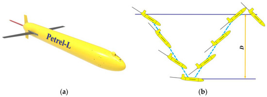
Figure 1.
The Petrel-L underwater glider and its working flow. (a) The Petrel-L underwater glider developed by Tianjin University, China. (b) The working flow of the Petrel-L underwater glider.

Table 1.
Technical specifications of Petrel-L.
When the Petrel-L starts working, it fixes itself by GPS and transmits the data to the base station via satellite. Then the oil is pumped from the external bladder into the inner oil box to adjust the buoyancy to dive. The wings will convert the vertical motion into forwarding motion within one profile period. The Petrel-L can adjust its heading and attitude underwater based on the pressure sensor and digital compass. When it reaches the preset depth D, the battery pack will move back, and the oil will be pumped back to the external bladder to achieve positive buoyancy for ascending. Afterwards, the Petrel-L climbs to the sea surface and moves the battery pack forward to obtain a better attitude for sending the data to and receiving commands from the base station via satellite. The working flow of Petrel-L is illustrated in Figure 1b.
2.2. Kinematic Model of Petrel-L
To comprehensively understand the motion of Petrel-L, a kinematic model is established, as shown in Figure 2. The kinematic parameters are crucial to the dead reckoning underwater and thus analyzed in detail. The relationship between the angular velocity and attitude of Petrel-L is described as follows:
where is the yaw angle, is pitch angle, is roll angle, and , , and denote the angular velocity corresponding to three attitude angles, respectively.
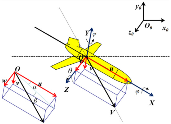
Figure 2.
The kinematic model of Petrel-L underwater glider.
Furthermore, the velocities of Petrel-L along the X, Y, Z axes in the geographic coordinate system are utilized to describe the following movement:
where u, v, and w are the velocity components along the axes in the body coordinate system.
Furthermore, the angle of attack α and the side slip angle β are deduced separately as follows:
3. Prediction Models
3.1. Regression Models
Regression is a technique used to model and analyze the relationship between UG control parameters and output parameters. Five regression models are utilized in our study, including linear regression, lasso regression, ridge regression, elastic net, and polynomial regression [21,22,23].
Linear regression (LR) attempts to model the relationship between dependent variables and independent variables using a linear approach. To reduce the influence of collinearity between the predicted variables, lasso regression (LAR) and ridge regression (RR) are proposed with L1-norm and L2-norm of linear regression. Furthermore, elastic net (EN) is a method that integrates the features of LAR and RR, which combines L1-norm and L2-norm as its penalty term. Polynomial regression (PR) is a special case of LR, which models a curvilinear relationship between two types of variables. However, PR is suited to deal with nonlinear and separable data and could achieve better parameters with prior knowledge, leading to overfitting.
3.2. Classical Machine Learning Models
Six classical machine learning models are also introduced in the study. The support vector regression (SVR) proposed by Harris in 1997 is an important branch of support vector machine (SVM) [24], which is commonly used in many areas [25,26,27]. The schematic of the SVR is shown in Figure 3a. The Gauss function is taken as the kernel function, which has better performance in large and small data sizes and fewer parameters than the polynomial kernel function. The back propagation neural network (BPNN) is the most rudimentary neural network, and its outputs and errors adopt forward propagation and back propagation, respectively [28]. The structure of BPNN is shown in Figure 3b, which contains three types of layers: the input layer, hidden layer, and output layer. K-nearest neighbor regression (KNNR) is a non-parametric statistical method for regression, and the input contains k closest training samples from feature space [29].
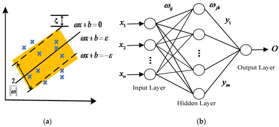
Figure 3.
The schematic of machine learning models. (a) The schematic of SVR [30]. (b) The structure of BPNN [31].
To address the problems of slow computation speed and low accuracy, the genetic algorithm (GA) and particle swarm optimization (PSO) are adopted to optimize the initialization for SVR and BPNN [30,31].
3.3. Tree-Based Models
In addition to the above prediction methods, tree-based models are also used for prediction, which also belong to machine learning. A decision tree (DT) is a kind of tree structure in which each internal node represents a judgment on an attribute. The random forest (RF) algorithm is an ensemble technique that combines multiple decision trees [32]. The structure of the RF is shown in Figure 4a. Furthermore, the advantages of the RF are that they are less sensitive to the outliers in the dataset and do not require much parameter tuning. Bagging (BG) is also an ensemble meta-algorithm, which can improve the stability and accuracy of machine learning algorithms [33]. In our study, we integrate bagging into DT methods to reduce the variance of DTs. A gradient boosting tree (GDBT) is an algorithm to classify or regress the data using an additive model such as the linear combination of basis, which can reduce the residual generated in the training process [34]. Adaptive boosting (Ada-Boost) uses the difference between the real value and predicted value of the previous learner to train the next learner, the point of which is to train the weak classifier iteratively and calculate their weight. The configuration of Ada-Boost is shown in Figure 4b. Extreme gradient boosting (XGBT) comes from the framework of gradient boosting [35].
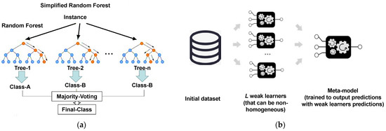
Figure 4.
The schematic of machine learning models. (a) The structure of RF [32]. (b) The configuration of Ada-Boost.
3.4. Simulated Annealing Optimized Frank–Wolfe Combination Model
The combination model is widely used in various fields, such as civil engineering, energy engineering, time series prediction, etc. [36,37,38]. To integrate the advantages of various models, the weight of single models should be calculated according to the prediction error. Then the sum of the square of the prediction error of a combination model is defined as the objective function to obtain the optimal weight for combination.
Supposing there are n single prediction models, define as Yit (i = 1,2, …n, t = 1,2, … N), Yt is tth observation value, then the common form of the combination model is
where ωi is the weight of the ith single prediction model, and ; et is the prediction error of the combination model.
Define the prediction error of the ith model as , then
So, the sum of the square of the prediction error of the combination model is
where .
Let
where E is prediction error information matrix and expressed as
Therefore, the mathematical programming model of optimal weight is determined as
where , denotes n dimensional matrix.
To solve the optimal weight of the combination model, the Frank–Wolfe method is introduced because it is suitable to solve the nonlinear problem in this study. Furthermore, to avoid falling into a local optimum while searching, the simulated annealing algorithm was used to optimize the Frank–Wolfe method. Pseudo-code of the SAFW algorithm to calculate the weight is shown in Algorithm 1.
| Algorithm 1: SAFW algorithm |
| Input: historical data → from glider flash 1: Divide the data into train set and test set 2: Import train data into single prediction model Yit (i = 1,2, …n, t = 1,2, …N) |
| 3: Test the data with the evaluation index (MSE and MAE) 4: Output eit → the prediction error of ith model, eit = eMAE + eMSE |
| 5: Calculate the error information matrix E |
| 6: Define initial weight and allowance error |
| 7: Solve Equation (10), and obtain the optimal solution U(k) |
| 8: if , 9: then stop the calculation and output W(k) |
| 10: else Start from W(k), and call SA for search; |
| 11: Add the variable to W(k) for search, then W(k+1) = + W(k) |
| 12: if f(W(k+1)) < f(W(k)) 13: then W = W(k) |
| 14: else Calculate the accepting possibility p = exp(−Δf/(kT)) |
| 15: Reach the iteration times, then |
| 16: Substitute in to , Output: λk |
| Return minimal prediction error J |
4. Experimental Results and Discussion
The experimental framework is shown in Figure 5 for a more specific description. The ocean current data imported from HYCOM is processed to meet the requirement first, which, together with the input parameters (preset heading, preset depth, preset buoyancy, preset pitch) of the sea trial data, are taken as the input train data sets. The output parameters (real heading, real distance) are taken as the output train data. Meanwhile, the average running period is about 4–5 h over one profile, so the data sets are divided into 50, 100, 200, and 300 groups corresponding to the time scales of 10, 20, 40, and 60 days. Afterwards, the data are trained by three types of prediction models, and 30 profiles are utilized for evaluation. Then the best methods are selected for distance and heading prediction with different data sizes, and all of them are integrated for a balanced and complete prediction of SPP.
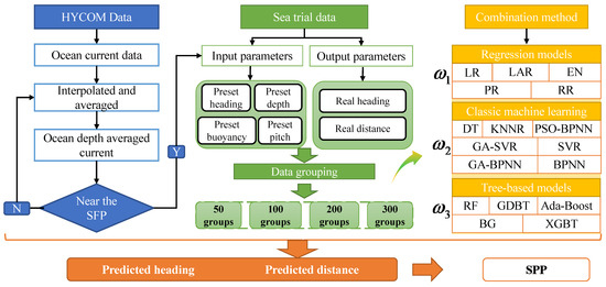
Figure 5.
The experimental framework of SPP prediction.
4.1. Data of Oceanic Depth-Averaged Current
To make the prediction more comprehensive and reliable, the ocean current data are downloaded from HYCOM in APDRC (Asia-Pacific Data Research Center). The data are updated every 24 h, and the resolution is 1/12°, which is lower than the average distance traveled by the UG during one profile. Therefore, the data should be processed to be close to the SPP of the UG. Figure 6 shows the sample data of eastward current velocity and northward current velocity in the sea trial area.
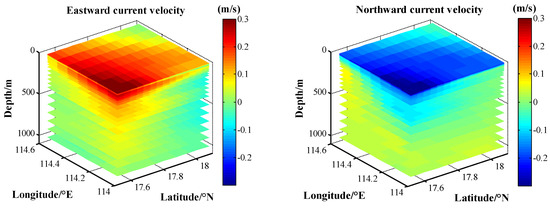
Figure 6.
The ocean current velocity in the sea trial area. (The sample data on 1 May 2019 were downloaded for website: http://apdrc.soest.hawaii.edu/las/v6/dataset?catitem=11458).
To guarantee ocean current data close to the ambient environment of the SPP, the IDW method is utilized to interpolate the downloaded data [39]. The IDW is widely used in various GIS analyses and adopts the distance weighted average of all local neighboring data points as the interpolated point. Furthermore, this method combines the advantages of both the Tyson polygon proximity method and the trend surface analysis method, thus having a better performance than other interpolation methods.
The IDW takes the distance between the sample point and the interpolation point as the weight, and the contribution of weight and distance is reversed. Consequently, the closer the interpolation point is, the greater the weight given to the sample point. The mathematical formula can be expressed as:
where Z is the estimated value of the interpolation point, Zi is the ith actual value, n is the number of samples involved in the interpolation, Di is the distance between interpolation point and the ith sample point, and m is the power of distance, which affects the interpolation results significantly. Generally, the default value of m is set to 2, considering the two-dimensional interpolating problem.
According to the working flow of Petrel-L, the single-layered ocean current cannot reflect the full impact of the environment. The oceanic depth-averaged current (ODAC) is adopted as a comprehensive ocean current related to the working depth of the UG, as shown below:
where d is the layer number of the ocean current, N is the maximum layer number corresponding to the actual working depth of the UG during one profile, UC is eastward ocean current velocity, and VC is northward ocean current velocity.
4.2. Sea Trial Data
The sea trials were conducted from 27 July 2019 to 23 April 2020. During the experiment, Petrel-L was equipped with a Glider Payload CTD sensor to acquire the salinity and temperature parameters in the interest areas. The deployment and recovery information of the UG is listed in Table 2. The sea trials lasted for 271 days without fault, 1051 profiles were acquired in total, and the total range was 4230.5 km. Here, the biofouling affection for the UG is ignored to simplify the data training process. The uncertainty of glider assembly and GPS are also ignored. Profiles 78–436 are selected as the research data, the initial parameters of the profiles are identical, which could avoid unnecessary influences from other sources. The sea trial areas of Petrel-L (CHC15) in the NSCS are shown in Figure 7, which shows the preset path and actual trajectory. The in-situ deployment and recovery pictures are also displayed by inset (1) and (2), respectively, in the left upper corner.
Table 2.
The deployment and recovery information of the UG.
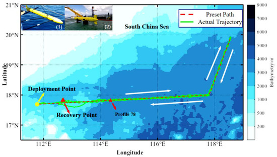
Figure 7.
The sea trial areas of the Petrel-L underwater glider (CHC15) in the NSCS. The yellow circle denotes the deployment point, and the red triangle denotes the recovery point. The red pentagram is Profile 78, which is selected as the start point of our data for the initial parameters that have been set as identical since then. The white arrows indicate the sailing direction of Petrel-L.
4.3. Data Analysis and Verification
According to the actual working parameters and information listed in Table 3, and part of the experiment data listed in Table 4, the SPP can be deduced from the distance and the heading relative to O and the last SPP. The real distance and heading data are shown in Figure 8. Taking the schematic shown in Figure 9 as a case study, the calculation formulae are given by:
where Olon and Olat are the longitude and latitude of the last SPP, respectively, L is the distance during one profile, and H is the heading of O.
Table 3.
The working parameters and information of the UG.
Table 4.
Part of the experimental data.
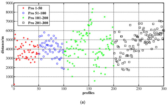
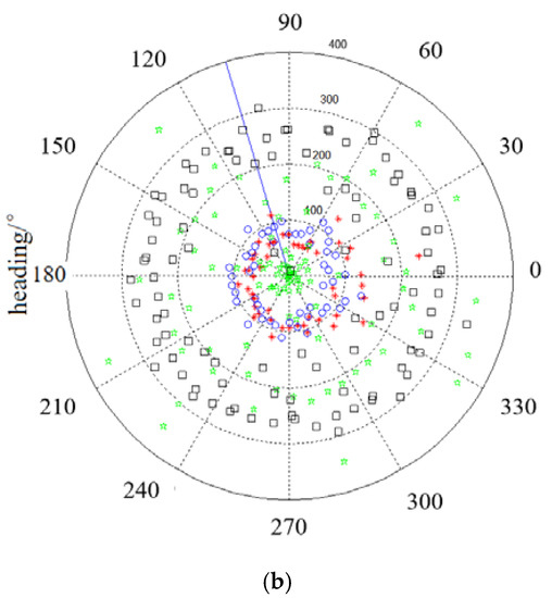
Figure 8.
The real distance and heading data required in the sea trial. (a) The distribution profile distance of the UG. (b) The distribution profile heading of the UG.
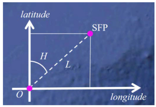
Figure 9.
The calculation schematic of the SPP.
We divided the data into four groups as 50, 100, 200, and 300 profiles after the data analysis and preprocessing. Due to sensor positioning errors and data drift, we preprocessed the original data. Abnormal data were raised and missing data were filled in. Each group corresponds to different time scales. Fifty profiles are roughly equivalent to 10-day data, 100 profiles to 20-day data, and so on. Afterwards, three kinds of prediction models were applied to each group of data for training, and 30 profiles were adopted as the test data. The results are shown in Figure 10, Figure 11, Figure 12 and Figure 13.
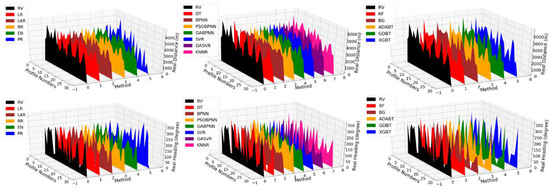
Figure 10.
Real distance and heading prediction with regression model (left), classical machine learning model (middle), and tree-based model (right) for 50 groups of data.
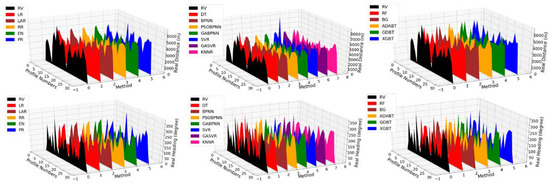
Figure 11.
Real distance and heading prediction with regression model (left), classical machine learning model (middle), and tree-based model (right) for 100 groups of data.
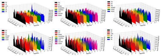
Figure 12.
Real distance and heading prediction with regression model (left), classical machine learning model (middle), and tree-based model (right) for 200 groups of data.
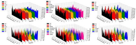
Figure 13.
Real distance and heading prediction with regression model (left), classical machine learning model (middle), and tree-based model (right) for 300 groups of data.
As shown in Figure 10, the predicted distance shows no dramatic change. Because the size of the 50-profile group data is relatively small, the regression model performs a little better than the other two models. Furthermore, for the real heading prediction, the LR, RR, LAR, and EN models take on more stable trends than the others. In Figure 11, when the data size grows to 100, the classical machine learning model shows relatively better performance in the heading prediction. However, there are some abnormal points in both the regression model and the tree-based model. Similarly, abnormal points appear in the regression model and machine learning model for distance prediction, and the tree-based model shows better prediction than them. Furthermore, Figure 12 and Figure 13 reveal that the classical machine learning model and tree-based model have a distinct advantage in predicting either heading or distance when the number of the data groups is over 200.
To make a specific evaluation of the prediction models, the MAE (mean absolute error), MSE (mean square error), and R2 (R-squared) are introduced as assessment indexes. The calculation formulae are shown as follows, respectively:
where yi is the real value, is the predicted value, and is the average value of all the real values. The evaluation results of the three models are shown in Figure 14 and Table 5 and Table 6.
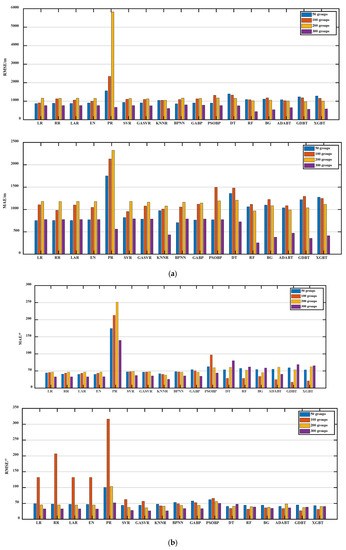
Figure 14.
Prediction error of real distance and heading prediction with three kinds of models. (a) Prediction error of real distance. (b) Prediction error and correlation of real heading.
Table 5.
Evaluation results of real heading with three types of methods.
Table 6.
Evaluation results of real distance with three types of methods.
As shown in Figure 14, Table 6 and Table 7, when the number of data groups is 50, the performance of the three models in distance prediction is not ideal. Among the regression models, LR, RR, and LAR perform better, and their MAE and MSE are comparable. EN and LAR perform well in heading prediction, and the MAE, MSE, and correlation coefficient of EN are 40.28 m, 47.05 m, and 0.76, respectively.
Table 7.
Weights of selected prediction models at different time scales.
When the data size increases to 100, the RF behaves better in distance prediction, and the GABPNN does well in heading prediction. Their prediction errors are smaller and take on a strong correlation when compared to the other models. As the number of data groups exceeds 200, the advantages of classical machine learning and tree-based model predictions become obvious gradually, and the prediction error decreases correspondingly. The GASVR outperforms the others in distance prediction, and the predicted correlation coefficients are 0.72 and 0.80, corresponding to 200 and 300 groups of data, respectively. Meanwhile, the BAG achieves better heading prediction results, with correlation coefficients of 0.63 and 0.72, corresponding to 200 and 300 groups of data, respectively. In addition, the PR does not perform well in the distance and heading prediction, especially when the amount of data groups is 100 and 200. According to its mathematical principle, the PR is suited to predictions with few variables, which is not suited to the multi-input single-output problem.
With the single models that predicted well at specified time scales, the combination model is derived based on the prediction error of selected single models. We adopted the simulated annealing optimized Frank–Wolfe method to calculate the weight of selected models. The detailed results are listed in Table 7, and the final prediction model for the SPP is expressed in Equation (12).
Additionally, the evaluation results of the real data with a combination model are shown in Figure 15 and Table 8. The MAEs and MSEs show a considerable level compared with the selected optimal single prediction models in distance and heading. Furthermore, the correlation coefficients of the combination model are better than the single prediction models, and it is higher in heading prediction than distance.
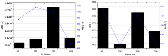
Figure 15.
Prediction error of real distance and heading prediction with proposed models.
Table 8.
Evaluation results of the combination model.
Overall, the experimental results indicated that the three types of single prediction models could show their advantages at different time scales with different data sizes. The regression model is more suited to short term prediction, achieving better results with less training data. As for a long-term prediction, the classical machine learning model is superior to the other models with data accumulation because its essence is suited to a large data size. Furthermore, the tree-based model can integrate the advantages of multiple models to a certain extent and perform well. Consequently, the weights of selected single models were calculated according to their prediction errors and integrated into them as a new combination model. After that, the prediction results of the combination model demonstrated that it has a balanced performance for distance and heading prediction at different time scales and outperforms other single models, because it integrated the advantages of single models with optimal weight.
5. Conclusions
In this paper, a new combination model was proposed to predict the SPP at different time scales. To make the prediction more accurate, the ocean current data are introduced as an ambient influence factor. Furthermore, the ocean current data are also interpolated and averaged to be closer to the ambient environment of the SPP. To make the analysis closer to reality, the sea trial data are then grouped into four sizes according to the different time scales of 10, 20, 40, and 60 days. Afterward, seventeen prediction models are categorized into regression models, classical machine learning models, and tree-based models for SPP prediction with different data sizes. The regression model is suited to dealing with linear problems and the machine learning model is good at processing big data problems. Finally, the prediction results reveal that the regression model is more suited to short-term predictions, whose MSE and RMSE are 751.40 m and 872.98 m in distance prediction, acquiring better results with small data sizes. Furthermore, when the number of data groups increases, the classical machine learning model performs better than other models. Similarly, the tree-based model also performs well, because it can integrate the strengths of multiple models to a certain degree in the long-term prediction. Furthermore, the combined weight is calculated based on the prediction error of three types of prediction models adopted by the simulated annealing optimized Frank–Wolfe method. Then various prediction models are combined with optimal weight to construct a new model for the SPP prediction of the UG, whose MSE and RMSE are 254.36 m and 445.02 m in distance. The combination prediction model shows high accuracy and balanced performance at different prediction time scales.
Further work will focus on the prediction of the underwater position of the UG with the predicted SPP. By considering target detection and the low cost of the UG, we will carry out the study of accurate dead reckoning of the UG without the inertial sensors. After that, a swarm control algorithm will be studied for the applications of multiple UGs, such as in ocean phenomenon reconstruction or regional marine environment detection.
Author Contributions
Conceptualization, R.Z. and S.Y.; methodology, D.X.; software, R.Z.; validation, Y.W., S.Y. and R.Z.; formal analysis, R.Z.; investigation, D.X.; resources, X.W.; data curation, Y.W.; writing—original draft preparation, R.Z.; writing—review and editing, D.X.; visualization, S.Y.; supervision, W.N.; project administration, W.N.; funding acquisition, W.N.. All authors have read and agreed to the published version of the manuscript.
Funding
This research was jointly funded by the National Key R&D Program of China; the National Natural Science Foundation of China (Grant No. 51721003); the Laoshan Laboratory Science and Technology Innovation Project (Grant No. LSKJ202200200); the Aoshan Talent Cultivation Program (Grant No. 2017ASTCP-OE01) of the Pilot National Laboratory for Marine Science and Technology (Qingdao); and the natural Science Foundation of Tianjin City (Grant No. 19JCQNJC03700).
Institutional Review Board Statement
Not applicable.
Informed Consent Statement
Not applicable.
Data Availability Statement
Not applicable.
Acknowledgments
The authors also would like to express their sincere thanks to L. Ma and J. Chen for their help in revising the grammar.
Conflicts of Interest
The authors declare no conflict of interest.
References
- Henry, S. The Slocum mission. Oceanography 1989, 2, 22–25. [Google Scholar]
- Zhang, R.; Yang, S.; Wang, Y.; Wang, S.; Gao, Z.; Luo, C. Three-dimensional regional oceanic element field reconstruction with multiple underwater gliders in the Northern South China Sea. Appl. Ocean Res. 2020, 105, 102405. [Google Scholar] [CrossRef]
- Ma, W.; Wang, Y.; Yang, S.; Wang, S.; Xue, Z. Observation of internal solitary waves using an underwater glider in the northern South China Sea. J. Coastal Res. 2018, 5, 1188–1195. [Google Scholar] [CrossRef]
- Dong, J.; Domingues, R.; Goni, G.; Halliwell, G.; Kim, H.-S.; Lee, S.-K.; Mehari, M.; Bringas, F.; Morell, J.; Pomales, L. Impact of assimilating underwater glider data on hurricane Gonzalo (2014) forecast. Weather Forecast. 2017, 32, 1143–1159. [Google Scholar] [CrossRef]
- Wu, D.; Zhao, Y.; Capozzi, B. Fundamental surface trajectory models for air traffic automation. In Proceedings of the Conference on 10th AIAA Aviation Technology, Integration, & Operations, Fort Worth, TX, USA, 13–15 September 2010. [Google Scholar]
- Best, G.; Fitch, R. Bayesian intention inference for trajectory prediction with an unknown goal destination. In Proceedings of the Conference on Intelligent Robots and Systems (IROS), Hamburg, Germany, 28 September–2 October 2015. [Google Scholar]
- Xie, G.; Gao, H.; Qian, L.; Huang, B.; Li, K.; Wang, J. Vehicle trajectory prediction by integrating physics- and maneuver-based approaches using interactive multiple models. IEEE Trans. Ind. Electron. 2018, 7, 5999–6008. [Google Scholar] [CrossRef]
- Quan, B.; Yang, B.; Hu, K.; Guo, C.; Qin, L. Prediction model of ship trajectory based on LSTM. Comput. Sci. 2018, 0z2, 126–131. [Google Scholar]
- Lin, Y.; Zhang, J.; Liu, H. An algorithm for trajectory prediction of flight plan based on relative motion between positions. Front. Inform. Techol. Electron. Eng. 2018, 7, 905–916. [Google Scholar] [CrossRef]
- Peng, X.; Zhang, B.; Zhou, H. An improved particle swarm optimization algorithm applied to long short-term memory neural network for ship motion attitude prediction. Trans. Inst. Meas. Control 2019, 15, 4462–4471. [Google Scholar] [CrossRef]
- Xiao, Z.; Li, P.; Havyarimana, V.; Hassana, G.M.; Wang, D.; Li, K. GOI: A novel design for vehicle positioning and trajectory prediction under urban environments. IEEE Sens. J. 2018, 18, 5586–5594. [Google Scholar] [CrossRef]
- Gao, H.; Su, H.; Cai, Y.; Wu, R.; Hao, Z.; Xu, Y.; Wu, W.; Wang, J.; Li, Z.; Kan, Z. Trajectory prediction of cyclist based on dynamic bayesian network and Long Short-Term Memory model at unsignalized intersections. Sci. China Inf. Sci. 2021, 64, 172207. [Google Scholar] [CrossRef]
- Ngo, P.; Al-Sabban, W.; Thomas, J.; Anderson, W.; Das, J.; Smith, R.N. An analysis of regression models for predicting the speed of a wave glider autonomous surface vehicle. In Proceedings of the Australasian Conference on Robotics and Automation, Sydney, NSW, Australia, 2–4 December 2013. [Google Scholar]
- Ngo, P.; Das, J.; Ogle, J.; Thomas, J.; Anderson, W.; Smith, R.N. Predicting the speed of a wave glider autonomous surface vehicle from wave model data. In Proceedings of the Conference on Intelligent Robots and Systems (IROS 2014), Chicago, IL, USA, 14–18 September 2014; pp. 2250–2256. [Google Scholar]
- Anitha, E.B.; Duraiswamy, K. A new hybrid approach for prediction of moving vehicle location using particle swarm optimization and neural network. J. Theor. Appl. Inform. Technol. 2014, 3, 791–800. [Google Scholar]
- Shen, X.; Zheng, Y.; Zhang, R. A hybrid forecasting model for the velocity of hybrid robotic fish based on back-propagation neural network with genetic algorithm optimization. IEEE Access 2020, 8, 111731–111741. [Google Scholar] [CrossRef]
- Havyarimana, V.; Hanyurwimfura, D.; Nsengiyumva, P.; Xiao, Z. A novel hybrid approach based-SRG model for vehicle position prediction in multi-GPS outage conditions. Inform. Fusion 2017, 41, 1–8. [Google Scholar] [CrossRef]
- Chassignet, E.P.; Hurlburt, H.E.; Smedstad, O.M.; Halliwell, G.R.; Hogan, P.J.; Wallcraft, A.J.; Baraille, R.; Bleck, R. The HYCOM (HYbrid Coordinate Ocean Model) data assimilative system. J. Marine Syst. 2007, 65, 60–83. [Google Scholar] [CrossRef]
- Yang, M.; Wang, Y.; Wang, S.; Yang, S.; Song, Y.; Zhang, L. Motion parameter optimization for gliding strategy analysis of underwater gliders. Ocean Eng. 2019, 191, 106502. [Google Scholar] [CrossRef]
- Wang, Y.; Yang, S. Glider. In Encyclopedia of Ocean Engineering; Cui, W., Fu, S., Hu, Z., Eds.; Springer: Singapore, 2019; pp. 1–12. [Google Scholar]
- Hoerl, A.E.; Robert, W.K. Ridge regression: Biased estimation for nonorthogonal problems. Technometrics 1970, 1, 55–67. [Google Scholar] [CrossRef]
- Tibshirani, R. Regression shrinkage and selection via the lasso. J. R. Stat. Soc. Ser. B. 1996, 1, 267–288. [Google Scholar] [CrossRef]
- Zou, H.; Trevor, H. Regularization and variable selection via the elastic net. J. R. Stat. Soc. Ser. B 2005, 2, 301–320. [Google Scholar] [CrossRef]
- Zhu, M.; Hahn, A.; Wen, Y.-Q.; Sun, W.-Q. Optimized Support vector regression algorithm-based modeling of ship dynamics. Appl. Ocean Res. 2019, 90, 101842. [Google Scholar] [CrossRef]
- Deng, H.; Liu, Y.; Li, P.; Zhang, S. Whole flow field performance prediction by impeller parameters of centrifugal pumps using support vector regression. Adv. Eng. Softw. 2017, 114, 258–267. [Google Scholar] [CrossRef]
- Zhang, H.; Wu, Q.; Li, F. Application of online multitask learning based on least squares support vector regression in the financial market. Appl. Soft. Comput. 2022, 121, 108754. [Google Scholar] [CrossRef]
- MMR Tabari, H.R.Z. Sanayei. Prediction of the intermediate block displacement of the dam crest using artificial neural network and support vector regression models. Soft. Comput. 2019, 29, 9629–9645. [Google Scholar] [CrossRef]
- Rumelhart, D.E.; Hinton, G.E.; Williams, R.J. Learning representations by back-propagating errors. Nature 1986, 6088, 533–536. [Google Scholar] [CrossRef]
- Jiang, L.; Xue, H.; Li, R.; Wu, J. A KNN composite-based piezoelectric helix for ultrasonic transcutaneous energy harvesting. Appl. Phys. Lett. 2022, 23, 120. [Google Scholar] [CrossRef]
- Khan, S.; Grudniewski, P.; Muhammad, Y.S.; Sobey, A.J. The benefits of co-evolutionary Genetic Algorithms in voyage optimisation. Ocean Eng. 2022, 245, 110261. [Google Scholar] [CrossRef]
- Li, G.; Chou, W. Path planning for mobile robot using self-Adaptive learning particle swarm optimization. Sci. China Inf. Sci. 2018, 5, 52204. [Google Scholar] [CrossRef]
- Regier, P.; Duggan, M.; Myers-Pigg, A.; Ward, N. Effects of random forest modeling decisions on biogeochemical time series predictions. Limnol. Oceanog. Methods 2022, 21, 40–52. [Google Scholar] [CrossRef]
- Abramowicz, K.; Sara, S.; Strandberg, J. Nonparametric bagging clustering methods to identify latent structures from a sequence of dependent categorical data. Comput. Stat. Data Anal. 2023, 177, 107583. [Google Scholar] [CrossRef]
- Su, S.; Li, W.; Garg, A.; Gao, L. An adaptive boosting charging strategy optimization based on thermoelectric-aging model, surrogates and multi-objective optimization. Appl. Energ. 2022, 312, 118795. [Google Scholar] [CrossRef]
- Chen, T.; Carlos, G. Xgboost: A scalable tree boosting system. In Proceedings of the 22nd ACM SIGKDD International Conference on Knowledge Discovery and Data Mining, San Francisco, CA, USA, 13 August 2017; pp. 785–794. [Google Scholar]
- Ren, Q.; Li, M.; Song, L.; Liu, H. An optimized combination prediction model for concrete dam deformation considering quantitative evaluation and hysteresis correction. Adv. Eng. Inform. 2020, 46, 101154. [Google Scholar] [CrossRef]
- Yin, J.; Zou, Z.; Feng, X. On-line prediction of ship roll motion during maneuvering using sequential learning RBF neural networks. Ocean Eng. 2013, 61, 139–147. [Google Scholar] [CrossRef]
- Oezger, M. Significant wave height forecasting using wavelet fuzzy logic approach. Ocean Eng. 2010, 37, 1443–1451. [Google Scholar] [CrossRef]
- Lu, G.; Wong, D. An adaptive inverse-distance weighting spatial interpolation technique. Comput. Geosci. 2008, 9, 1044–1055. [Google Scholar] [CrossRef]


Disclaimer/Publisher’s Note: The statements, opinions and data contained in all publications are solely those of the individual author(s) and contributor(s) and not of MDPI and/or the editor(s). MDPI and/or the editor(s) disclaim responsibility for any injury to people or property resulting from any ideas, methods, instructions or products referred to in the content. |
© 2023 by the authors. Licensee MDPI, Basel, Switzerland. This article is an open access article distributed under the terms and conditions of the Creative Commons Attribution (CC BY) license (https://creativecommons.org/licenses/by/4.0/).