Abstract
The Brazil–Malvinas Confluence (BMC) is one of the most complex oceanic areas in the Earth’s oceans and the prediction of high frequency structures tends to fail. The authors studied the BMC using Multiscale Ultrahigh Resolution (MUR) imagery for the Sea Surface Temperature (SST) to address why the predictions are not as good as expected. The studies were carried out by means of two approaches. The first approach is the non-linear fitting of a harmonic model keeping the frequencies as parameters pixel by pixel. The second approach is from fractal geometry. The three first q-order Rényi dimensions were computed. At the same time, an inverse fractal interpolation was carried out to compute the contraction factor. Both of them are related to the chaotic behavior of nature. This work has three relevant contributions. The correlation between the harmonic models and the SST data is quite poor in general, implying the low harmonicity, and low harmonic predictability, of the pixel-by-pixel time series. It is verified that the quasi-annual and quasi-semiannual waves have periods of about 420 and 210 days, respectively. The second one is the confirmation of the high complexity of the BMC area because the three Rényi dimensions are equal. This has the strong finding of the monofractality of the dynamic of the SST in the BMC. Finally, the contraction factor, one of the parameters of the fractal interpolation, is relatively high, implying the presence of highly complex internal structures in the SST temporal evolution.
1. Introduction
The Brazil–Malvinas Confluence Zone (BMC) is a high hydrodynamic high energetic region just off the coast of Argentina and Uruguay, in front of the mouth of Rio de la Plata, where the warm poleward Brazil Current and the cold equatorward Malvinas Current meet (Figure 1). Although the location of the BMC oscillates in latitudinal direction with an annual periodicity, the confluence occurs between 35 and 45 degrees south latitude and 50 to 70 degrees west longitude [1,2].
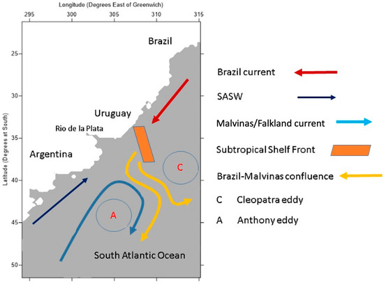
Figure 1.
Location of the area under study with a scheme of the relevant currents.
The Brazil Current is a warm poleward current of subtropical water. When the Atlantic South Equatorial Current meets the South America continent (around 10° S–15° S), it splits in two branches near Cabo de São Roque [2]. One flows northward, the North Brazil Current, through the Lesser Antilles and getting in the Caribbean Sea, and the other flows poleward along the Brazil coast. This last branch divides in two more at about 22° S. One of them flows eastward to establish the South Atlantic Gyre and the other one flows poleward along the South American continental shelf. This last can have temperatures between 18 and 28 °C, decreasing poleward [1,3,4].
The poleward Brazil Current, the South Atlantic Current, the Benguela Current, and the South Equatorial Current constitute the South Atlantic subtropical gyre. The separation of the Brazil Current from the coast is observed at about 38° S, then the southern boundary of the South Atlantic subtropical gyre is established. This area also oscillates in latitude and depending on how intense the Malvinas Current is; higher intensity, lower latitude [5,6,7,8].
The Malvinas or Falkland Current is a branch of the Antarctic Circumpolar Current, or West Wind Drift, after flowing through the Drake Passage. It flows equatorward along the Argentinian coasts, carrying cold subantarctic water. The Malvinas Current is not a surface current like the Brazil Current, but extends all the way to the sea floor. It is usual to find temperatures of about 6 °C [2]. The Brazil current and the Malvinas and the Sub-Antarctic Shelf Water (SASW) Current meet in the Argentinian Sea, in front of Rio de la Plata, in the Brazil–Malvinas Confluence, giving that area a mild climatic condition [9].
The surface flow, deduced from the Sea Surface Temperature (SST) imagery, is very complex and a more complete view comes from artificial satellites. The Brazil Current meets the Malvinas Current at about 38° S. An eddy at depth, named Anthony, occurs. Then, the Brazil Current splits in two branches. One gets redirected equatorward and it creates an anticyclonic eddy, Cleopatra. The other one deflects 45° eastward. On the other hand, when the Malvinas Current meets the Brazil Current, it is redirected poleward, joining again to the Antarctic Circumpolar Current [3,4,10,11].
The temperature in the BMC presents high gradients and the meanders, eddies, and filaments exist in different temporal and spatial scales [11,12,13,14]. The eddies are extremely energetic, leading to strong mixing as happens in Cleopatra and Anthony.
The BMC has been studied by means of classical oceanographic surveys [3,4], by GeoSat altimetry data [5], and by satellite sea surface imagery [13,15]. There are well-known global models and local inverse models [3,4], all of them based on experimental data. However, from the point of view of dynamical systems, the only reference known by the authors is [16]. These authors applied the Fisher–Shannon formalism to compute the Shannon Entropy as a measure of the order-disorder of the whole dynamic system of the BMC.
Now, the authors use three years and nine months (January 2016 to August 2019) of daily SST Multiscale Ultrahigh Resolution imagery assuming the SST as a tracer of the dynamic of the upper layer of the ocean. The first study is about the harmonicity of the time series in each point of the domain. The spatial distributions of the amplitude, phase lag, and frequency of the annual and semiannual waves are analyzed. A first important result is that it is more correct to talk about quasi-annual and quasi-semiannual waves because their periods are close to 420 and 210 days, respectively. Considering the time series of SST of each pixel as the result of a dynamical system to give way to the Fractal Geometry, the second study consists of computing the three firsts order Rényi following [17,18,19,20,21]. A second important result is that most of the area has a high fractal dimension, according to the results of [16]. The now very important result is that the three Rényi dimensions are equal, being monofractal. Finally, the computation of the parameters of a fractal linear interpolation model led to a relatively high contraction parameter. All the results are in agreement with the conclusions of [16].
The organization of the work is as follows. Section 2 is devoted to the description of the datasets and to an outline of the non-linear quasi-harmonic interpolation, fractal interpolation, and fractals dimensions. Results are presented in Section 3. Finally, the discussion and conclusions are drawn in Section 4.
2. Dataset and Numerical Methods
2.1. Data
The Multiscale Ultrahigh Resolution (MUR) imagery is produced by the National Aeronautics and Space Administration at the Jet Propulsion Laboratory. MUR is a global SST analysis field produced daily on a 0.01°·0.01° grid with an equatorial spatial resolution of 1.1132 km. MUR joins the products of multiple satellite mission datasets at different resolutions over multiple different time scales. The method used to combine the different spatial and temporal resolutions satellite imagery is the multiresolution variational analysis based on a specified wavelet basis. MUR takes the SST imagery of the Aqua/MODIS, Aqua/AMSR-E, CORIOLIS/WINDSAT, Terra/MODIS, NOAA-19/AVHRR-3, and GCOM-W1/AMSR2 missions and sensors together in in situ datasets [22]. For the purposes of this work, the authors used the daily Level 4 MUR imagery between the coordinates [294° W, 20° S]–[315° W, 51° S] and spanning since 1 January 2016 to 31 August 2019, with a total of 1419 SST fields and more than 280,000 points with SST ocean data.
As an example, the mean SST field and the standard error in its estimation are shown in Figure 2a,b, respectively. Following Figure 2a and comparing it with Figure 1, the Brazil Current is easily guessed as a warm yellow tongue running parallel to the coast and poleward. Close to the coast, about 33° S, the Subtropical Shelf Front is guessed by the sudden change of color. The darkest areas correspond to the eastward meanders after the encounter of the equatorward Malvinas and Sub-Antarctic Surface Water (SASW) with the Brazil Current just at the south of the mouth of the Rio de la Plata with about 6 °C. The location of Cleopatra (see Figure 1) is easily guessed. Anthony is not seen because it mainly happens at depth.

Figure 2.
(a) Mean SST in degrees Celsius degrees; (b) error in the estimation of the SST in degrees Celsius. The higher errors are concentrated near the mouth of Rio de la Plata.
The error in the estimation of the mean temperature (Figure 2b) shows close to zero values with points with anomalous higher values that will be explained further. Basically, the points with highest values are in the area of confluence of currents and where the water escapes eastward.
It could be said that there are some inconsistences in where the location of Cleopatra or the confluence are. In this sense, it has been reported a North–South and East–West seasonal displacement of the confluence area and of all related structures [23]. Therefore, Figure 2a shows the average SST field, and the average location for the studied time span of the Brazil–Malvinas Confluence.
2.2. Numerical Techniques
2.2.1. Nonlinear Fit Quasi-Harmonic Model
Every time series of the SST of each pixel was submitted to a nonlinear Levenberg–Marquardt least squares on the theoretical model:
where is the mean value in Celsius degrees, the first component (subindex 1) is the annual and the second one (subindex 2) is the semiannual. The cosine and sine amplitudes of both are also in degrees Celsius degrees. Frequencies are written in radians/day. The amplitude and phase of each component are recovered, respectively, by
A nonlinear least square fit is used because frequencies will be parameters to fit. There are not too many needs for considering a frequency varying quasi-annual component, but because the climatic exogenous bearings used to have periods around six month long, the semiannual component must be considered, and its frequency is considered a parameter to fit too. The nonlinear fit is very sensitive to the initial estimation. The best choices have to be in the range of the time series data for the mean temperature, the half range and a quarter of the range for the cosine and sine amplitudes, respectively, and 2π/365 or 180 for the frequencies of the annual and semiannual components.
2.2.2. Iterated Function System: Fractal Interpolation
A fractal set can be submitted to geometrical transformations [24,25]. An affine transformation to perform translation, stretching, and rotation on a given set [26,27,28]. The special case of two-dimensional affine transform is written in terms of:
For the purposes of the Iterated Function System at the time to be applied on discrete sequences, the coefficient b is set to zero. Therefore,
eliminating the rotation from the model of Equation (3). Equation (4) is an affine map that is called a shear transformation because horizontal lines are stretching by a factor of a and vertical lines by a factor of d, named the contraction factor for the map [25].
Equation (4) is constrained for the following two conditions on the end points of a N long data sequence:
The Direct Approach: Fractal Construction
A fractal set can easily be built by using the Iterated Function System as follows. Once the coefficients {a,c,d,e,f} have been fixed, the affine map of Equation (3) is applied on the coordinates of the attractor. A new set of coordinates is then obtained and the affine map of Equation (3) is applied again and again on all the new points. Thus, the affine map is iterated and the fractal is built [26,27,28].
If several attractors and several affine maps are defined, it is possible to build up really complex fractal sets in a very easy way as happens with the Barnsley’s fern. This consists of four affine maps on four attractors. More iterations, more complexity.
The inverse approach: fractal interpolation function
In linear fractal interpolation, a set of interpolation points is interpolated by means of a continuous single valued function that passes through the interpolation points [26,27,28]. Here, the idea is to build up an affine transform to find the coefficients for Equation (2) such that when iterated, it reproduces the data sequence to be modeled [26,27,28].
Following [26], the least square estimators of the set of parameters [a,c,d,e,f] are:
for each interpolating interval [i − 1, i] inside the whole length of the series [0, M]. The contraction coefficient, d, is computed as follows. First, compute the weight for the numeral n inside the interval with order F (Final) and I (Initial).
Then, compute the functions An and Bn for each numeral:
Finally,
With the same constraints of Equation (5).
If there are several intervals in the same time series, then a number of contraction factors will be obtained and by the Theorem of Collage [27,28], the value of the contraction factor will be the average of all the contraction factors.
However, the inverse approach in linear fractal interpolation can be carried out if the discrete data to be modeled are self-affine or self-similar or piece-wise self-affine [29].
2.2.3. Fractal Dimensions
Following [24,25], a fractal is an object with a dimension different from its topological one. A point is zero dimensional, the infinite line is one dimensional, a surface is two dimensional, etc. However, there are objects with non-integer dimension such as the Cantor set, the Sierpinski triangle, a snowflake, etc. The parameter to express how an object fills the space arises from the halfway point of the Geometric Theory of the Measure and the Fractal Geometry and it is named fractal dimension. The most intuitive way is for the case of two and three dimensions. The space where the object is it is covered by a ε-blanket, say squares/cubes of sides ε long. The squares/cubes, partially or fully occupied by the object, are counted and the dimension is computed as [24,25]:
This is known as box-counting dimension, box dimension, Minkowski dimension, packing dimension, and most of the time coincides with the Hausdorff dimension [24,25].
A different problem is when measuring the strangeness of strange attractors. These occur in dynamical systems and their outputs are a time series. The dimension of the attractor will be a measure of its strangeness. In [30,31], it was demonstrated that a pure harmonic time series is the result of a zero-dimensional attractor working with time series from superconducting gravimeters, relating it with the dynamic on a line around the attractor and that this idea was not followed by ocean tides.
Refs. [17,18,19,20] derived an expression for the computation of the strangeness of an attractor in dynamical systems changing the number of squares/cubes for the number of correlated orbits. Ref. [21] gave the way to compute dimensions using orbits. The correlation integral is approached by:
where N is the number of orbits once the embedding dimension, m, has been fixed, xi is the i-thm orbit and θ(·) is the step or Heaviside function. Equation (10) is the discrete version of the correlation integral
The dimension is computed as
However, for a general computation of all possible dimensions:
grouped under the name of order-q Rényi dimensions or order-q dynamical entropies [32,33]. When Dq is independent of the value of q, the object is called monofractal, otherwise, it will be multifractal.
When q = 0, it is named fractal dimension or Hausdorff dimension; when q = 1, it is called information dimension; and when q = 2, it is the correlation dimension. The fractal dimension is read as above. The information dimension is read as a measure of the fractal dimension of an unknown probability distribution. At the same time, it is a way to characterize the growth rate of the Shannon entropy, in connection to [16]. The correlation dimension is what determines the dimension of fractal object. Following [31], the attractor is super-attractive if the correlation dimension is zero, attractive if its value is between zero and one, indifferent if it is equal to unity and repulsive if it is greater than one.
A comment is necessary on the embedding dimension and the delay. Following [24], the embedding dimension is, roughly speaking, the length of orbits, or the length of a piece of orbit. The value of the embedding dimension must be related to the periods in the time series. If a daily time series has periods of one year and six months in, a good choice can be orbits of length 30 or 60, never greater than one third of the shorter period. This criterion is similar to that used in power spectral analysis for the maximum number of frequency bands. Concerning the delay, this is the number of data points, the difference in time, between two successive orbits. For the purposes of this work, the delay is 30 days, so the orbits do not share data. In this case, this choice does not present problems because of the proportionality of the periods of the two considered harmonic components.
3. Results and Discussion
3.1. Nonlinear Fit Quasi-Harmonic Model
The coefficient of determination from the application of the non-linear fitting of Equation (1) on the SST of each pixel (Figure 3) presents low values, lower than 0.75, where the confluence is located in front of mouth of the Rio de la Plata. Comparing Figure 3 with Figure 1, the poleward path of the Brazil Current is easily guessed and the eastward paths of the Brazil–Malvinas confluence as well. The circular area of lower coefficient of determination leads us to think that Cleopatra has moved, but it is the area where the Malvinas and Brazil currents meet and the important contribution from the Rio de la Plata pushes them eastward [8,9].

Figure 3.
Coefficient of determination of the nonlinear fit (Equation (14)).
Now the spatial structure of the mean SST field becomes clearer (Figure 2a,b). The points with higher errors in the estimation of the mean value (Figure 2b) correspond to the lower values in the coefficient of determination, just in front of the mouth of the Rio de la Plata.
The spatial distributions of the amplitude, frequency, and phase lag of the annual component are presented in Figure 4 together with their respective errors in the estimation. The anomalous values in Figure 4 and Figure 5 are artifacts due to the high sensitivity of the non-linear regression to the errors. The paths of the Brazil and Malvinas currents amplitude of the annual component (Figure 4a) are easily guessed by the 10–12 °C strips. The areas with negative values mean a change in the sign of the phase lag. Those places with very high values of the annual amplitude correspond to places with low determination coefficient. The errors in the estimation of the amplitude of the annual component (Figure 4b) are close to zero.
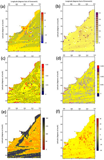
Figure 4.
Spatial distribution of the (a) amplitude of the annual component in degrees Celsius; (b) error in the estimation in degrees Celsius; (c) frequency from the nonlinear least squares fit in rad/day; (d) error in the estimation of the frequency; (e) phase lag in degrees; (f) error in the estimation of the phase in degrees.
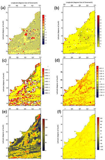
Figure 5.
Spatial distribution of the (a) amplitude of the semiannual component in degrees Celsius; (b) error in the estimation in degrees Celsius; (c) frequency from the nonlinear least squares fit in rad/day; (d) error in the estimation of the frequency; (e) phase lag in degrees; (f) error in the estimation of the phase in degrees.
The frequency of the annual wave (0.0172 rad/s) is well kept in the area of study (Figure 4c). However, it seems that it could be more correct talking about a quasi-annual wave or component because the period of about 415 days is the most frequent. The error in the estimation of the frequency is close to zero except in front of the mouth of Rio de la Plata and where Cleopatra is located (see Figure 1).
The spatial distribution of the phase lag (Figure 4e) is similar to the amplitude (Figure 4a) with strips of close to zero phase lag in the paths of the Brazil and Malvinas Currents and rest of the area under study with a phase lag of about 120°, always referring to the time of the first image. The error in the estimation (Figure 4f) is close to zero except in the same places pointed out before, just in from of the mouth of Rio de la Plata.
The semiannual component presents a quite homogeneous value in its amplitude (Figure 5a). However, at the area in front of the mouth of Rio de la Plata, where all the currents meet, the amplitude increases notably but the determination coefficient is close to zero, hence it is meaningless. The error in the estimation is uniform and close to zero (Figure 5b).
Now the main problem on the semiannual wave is its frequency (Figure 5c). The semiannual wave has a frequency of 0.0349 rad/s. The path of the Brazil Current presents a period of about 210 days and there are many points with unreasonable values of fitted frequencies. The errors in its estimation (Figure 5d) are very high. The spatial pattern of the phase lag of the semiannual wave (Figure 5e) follows the scheme of the circulation (Figure 1). Cleopatra is easily guessed. Its error in the estimation is close to zero (Figure 5f). The number of points with anomalous values is higher than with the annual component.
3.2. Fractal Dimensions
Following [17,18,19,20,21], the fractal dimensions Dq, with q = 0, q = 1, and q = 2, or Rényi dimensions, for the embedding dimensions of m = 30 and m = 60, are presented in Figure 6.
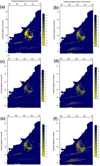
Figure 6.
Fractal or Hausdorff dimensions: (a) for embedding dimension of 30; (b) for embedding dimension of 60; (c) information dimension for the embedding dimension of 30; (d) as (c) but for the embedding dimension of 60; (e) correlation dimension for the embedding dimension of 30; (f) as (e) but for the embedding dimension of 60.
It is remarkable that the spatial distribution and the values of the three fractal dimensions (Dq, q = 0, 1, 2) are practically equal. This means that the area has the behavior of a monofractal [22,23]. Where the Brazil and Malvinas Currents meet, in from of the mouth of Rio de la Plata, has a dimension close to 1 and the rest a dimension close to 2.
3.3. Linear Fractal Interpolation
The fractal measures must finish with the application of the inverse modeling for the Fractal Interpolation Function. Following [26,27,28,29], the contraction factor is presented in Figure 7. Its value is quite constant in all the areas under study keeping the structure of the pattern of circulation of Figure 1. Higher value, higher contraction, higher variability, and higher errors, as can be seen from the comparison of Figure 2, Figure 3, Figure 4, Figure 5, Figure 6 and Figure 7.
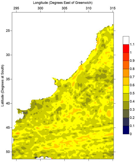
Figure 7.
Contraction coefficient from the linear fractal interpolation.
4. Conclusions
The area of the Brazil Current and Malvinas Current meet is very complex with many meanders, eddies and filaments. Following [25], it is affected by the annual component and the influence of the climate acts on the semiannual.
A quasi-harmonic model of two waves to compute the mean SST field, the amplitudes, frequencies, and phase lags of the annual and semiannual waves (Equation (14)) was fitted on the 1419 data time series of each one of the 400,000 pixels of ocean SST. The first important result is that it is more convenient to talk about of quasi-annual and quasi-semiannual components. The mean periods are about 420 and 210 days, respectively. The mean SST, amplitude, frequency, and phase lag fields follow the general scheme of surface circulation of the area. The most sensitive parameter is the frequency of the semiannual component. It presents high errors in estimation, errors that are propagated and that affect the rest of the parameters of the model of Equation (14). This is in accordance with [25] concerning the annual wave.
The second important contribution comes from assuming that each one of the time series of each pixel is the result of a dynamical system to give way to the Geometrical Theory of Measures. In [16], the Fisher–Shannon information and the Shannon entropy were computed and leading to reinforce the idea of the high complexity of the area. Now, the authors have computed the three firsts order Rényi dimensions [32] following [17,18,19,20]. According to [16], the dimension of the area in front of the mouth of Rio de la Plata is close to 1 and the rest of the field has a dimension close to 2, confirming the high complexity. However, the first very important contribution is that the three first Rényi dimensions are almost equal. This means that the whole area under study is a monofractal [22,23] because it seems to be only one model with a single type of output and not with multiple outputs. In other words, the SST time series are not multifractals, there are not multiple time scales in following progressive rescaling or self-similarity. Finally, the fourth conclusion comes from the computation of the fractal interpolation function on each time series. The contraction factor is quite homogeneous in the domain, reinforcing the idea of monofractality.
Author Contributions
Conceptualization, J.J.A. and J.M.V.; methodology, J.J.A. and E.B.; software, J.J.A., J.M.V. and E.B.; validation, J.J.A., J.M.V. and E.B.; formal analysis, J.J.A. and J.M.V.; investigation, J.J.A., J.M.V. and E.B.; resources, J.J.A., J.M.V. and E.B.; data curation, J.J.A., J.M.V. and E.B.; writing—original draft preparation, J.J.A.; writing—review and editing, J.J.A.; visualization, J.J.A., J.M.V. and E.B.; supervision, J.J.A.; project administration, J.M.V.; funding acquisition, J.J.A. and J.M.V. All authors have read and agreed to the published version of the manuscript.
Funding
This research has received funding from RNM160 and Interrreg-ATLAZUL (0755_ATLAZUL_6_E, POCTEP).
Data Availability Statement
Not applicable.
Conflicts of Interest
The authors declare no conflict of interest. The funders had no role in the design of the study; in the collection, analyses, or interpretation of data; in the writing of the manuscript; or in the decision to publish the results.
References
- Gordon, A.L. Brazil-Malvinas Confluence-1984. Deep Sea Research Part A. Oceanogr. Res. Pap. 1989, 36, 359363–361384. [Google Scholar] [CrossRef]
- Talley, L.D.; Pickard, G.L.; Emery, W.J.; Swift, J.H. Descriptive Physical Oceanography: An Introduction, 6th ed.; Academic Press: Burlington, MA, USA, 2011; p. 555. [Google Scholar]
- Orúe-Echevarría, D.; Pelegrí, J.L.; Machín, F.; Hernández, A.; Emelianov, M. Inverse Modeling the Brazil-Malvinas Confluence. J. Gephys. Res. Ocean 2019, 124, 527–554. [Google Scholar] [CrossRef]
- Orúe-Echevarría, D. The Brazil-Malvinas Confluence: From Local to Global Scales. Ph.D. Thesis, Universitat Politècnica de Catalunya, Barcelona, Spain, 2019. [Google Scholar]
- Chelton, D.B.; Schlax, M.G.; Witter, D.L.; Richman, J.G. Geosat altimeter observations of the sea surface circulation of the southern ocean. J. Geophys. Res. 1990, 95, 17887–17903. [Google Scholar] [CrossRef]
- Chelton, D.B.; Wentz, F.J. Global Microwave Satellite Observations of Sea Surface Temperature for Numerical Weather Prediction and Climate Research. Bull. Am. Meteorol. Soc. 2005, 86, 1097–1115. [Google Scholar] [CrossRef]
- Matano, R.P. On the separation of the Brazil Current from the coast. J. Phys. Oceanogr. 1993, 23, 79–90. [Google Scholar] [CrossRef]
- Piola, A.R.; Matano, R.; Palma, E.; Moller, O., Jr.; Campos, E. The influence of the Plata River discharge on the western South Atlantic shelf. Geophys. Res. Lett. 2005, 32, 1603–1606. [Google Scholar] [CrossRef]
- Piola, A.; Martinez, N.; Guerrero, R.; Jardón, F.; Palma, E.; Romero, S. Malvinas-slope water intrusions on the northern Patagonia continental shelf. Ocean Sci. 2010, 6, 345–359. [Google Scholar] [CrossRef]
- Stramma, L.; Ikeda, Y.; Peterson, R.G. Geostrophic transport in the Brazil Current region north of 20 °S. Deep-Sea Res. 1990, 37, 1875–1886. [Google Scholar] [CrossRef]
- Peterson, R.G.; Stramma, L. Upper-level circulation in the South Atlantic Ocean. Prog. Oceanogr. 1990, 26, 1–73. [Google Scholar] [CrossRef]
- Pilo, G.S.; Mata, M.M.; Azevedo, J.L.L. Eddy surface properties and propagation at Southern Hemisphere western boundary current systems. Ocean Sci. 2015, 11, 629–641. [Google Scholar] [CrossRef]
- Telesca, L.; Pierini, J.O.; Lovallo, M.; Santamaría-del-Angel, E. Spatio-temporal variability in the Brazil-Malvinas Confluence Zone (BMCZ), based on spectroradiometric MODIS-AQUA chlorophyll-a observations. Oceanologia 2018, 60, 76–85. [Google Scholar] [CrossRef]
- Mason, E.; Pascual, A.; Gaube, P.; Ruiz, S.; Pelegrí, J.; Delepoulle, A. Subregional characterization of mesoscale eddies across the Brazil-Malvinas Confluence. J. Geophys. Res. Ocean. 2017, 122, 3329–3357. [Google Scholar] [CrossRef]
- Piola, A.; Romero, S.; Zajaczkovski, U. Spacetime variability of the Plata plume inferred from ocean color. Cont. Shelf Res. 2008, 28, 1556–1567. [Google Scholar] [CrossRef]
- Pierini, J.O.; Lovallo, M.; Gómez, E.A.; Telesca, L. Fisher–Shannon analysis of the time variability of remotely sensed sea surface temperature at the Brazil-Malvinas Confluence. Oceanologia 2016, 58, 187–195. [Google Scholar] [CrossRef]
- Grassberger, P.; Procaccia, I. Characterization of Strange Attractors. Phys. Rev. Lett. 1983, 50, 346–349. [Google Scholar] [CrossRef]
- Grassberger, P.; Procaccia, I. Measuring the Strangeness of Strange Attractors. Phys. D Nonlinear Phenom. 1983, 9, 189–208. [Google Scholar] [CrossRef]
- Grassberger, P. Generalized Dimensions of Strange Attractors. Phys. Lett. A 1983, 97, 227–230. [Google Scholar] [CrossRef]
- Grassberger, P.; Procaccia, I. Dimensions and Entropies of Strange Attractors from a Fluctuating Dynamics Approach. Physica 1984, 13, 34–54. [Google Scholar] [CrossRef]
- Takens, F. Detecting Strange Attractors in Turbulence, Lecture Notes in Mathematics; Rand, D.A., Young, L.S., Eds.; Springer: Berlin/Heidelberg, Germany, 1981. [Google Scholar]
- Crosman, E.; Vázquez-Cuervo, J.; Chin, T.M. Evaluation of the Multi-Scale Ultra-High Resolution (MUR) Analysis of Lake Surface Temperature. Remote Sens. 2017, 9, 723. [Google Scholar] [CrossRef]
- Wainer, I.; Gent, P.; Goni, G. Annual Cycle of the Brazil-Malvinas confluence region in the National Center for Atmospheric Research Climate System Model. J. Geophys. Res. 2000, 105, 26167–26177. [Google Scholar] [CrossRef]
- Falconer, K. Techniques in Fractal Geometry; John Wiley and Sons: Hoboken, NJ, USA, 1997; ISBN 0-471-95724-0. [Google Scholar]
- Falconer, K. Fractal Geometry: Mathematical Foundations and Applications; John Wiley and Sons: Hoboken, NJ, USA, 2014; ISBN 111994239X. [Google Scholar]
- Mazel, D.S.; Hayes, M.H. Using Iterated Function System to Model Discrete Sequences. IEEE Trans. Signal Process. 1992, 40, 1724–1734. [Google Scholar] [CrossRef]
- Barnsley, M.F.; Ervin, V.; Hardin, D.; Lancaster, J. Solution of an inverse problem for fractals and other sets. Proc. Natl. Acad. Sci. USA 1986, 83, 1975–1977. [Google Scholar] [CrossRef] [PubMed]
- Barnsley, M.F.; Harrintong, A.N. The Calculus of Fractal Interpolation Functions. J. Approx. Theory 1989, 57, 14–34. [Google Scholar] [CrossRef]
- Rinaldo, R.; Zakhor, A. Inverse and Approximation Problem for Two Dimensional Fractal Sets. IEEE Trans. Signal Process. 1994, 3, 802–820. [Google Scholar] [CrossRef]
- Alonso, J. On the fractal dimension of Earth Tides and characterizations of gravity stations. Bull. D’inf. Des Marees Terr. 1998, 129, 9963–9973. [Google Scholar]
- Alonso, J.; Villares, P.; González, M.J.; Arias, M.; Marín, B. Ocean Tides and Fractal Geometry: Tidal Station Stability. Thalassas Int. J. Mar. Sci. 2005, 21, 9–16. [Google Scholar]
- Rényi, A. On the dimension and entropy of probability distributions. Acta Math. Acad. Sci. Hung. 1959, 10, 193–215. [Google Scholar] [CrossRef]
- Cover, T.M.; Thomas, J.A. Elements of Information Theory, 2nd ed.; Wiley: Hoboken, NJ, USA, 2012; ISBN 9781118585771. [Google Scholar]


Disclaimer/Publisher’s Note: The statements, opinions and data contained in all publications are solely those of the individual author(s) and contributor(s) and not of MDPI and/or the editor(s). MDPI and/or the editor(s) disclaim responsibility for any injury to people or property resulting from any ideas, methods, instructions or products referred to in the content. |
© 2023 by the authors. Licensee MDPI, Basel, Switzerland. This article is an open access article distributed under the terms and conditions of the Creative Commons Attribution (CC BY) license (https://creativecommons.org/licenses/by/4.0/).