A LSSVR Interactive Network for AUV Motion Control

Abstract

In view of the requirements on control precision of autonomous underwater vehicles (AUVs) in different operations, the improvement of AUV motion control accuracy is the focus of this paper. In regard to the unsatisfying robustness of traditional control methods, an interactive network based on Least Square Support Vector Regression (LSSVR) is therefore put forward. The network completed the identification of the strong nonlinear AUV dynamic characteristics based on the LSSVR theory and by virtue of the interactions between the offline and online modules, it achieved offline design and online optimization of the AUV control law. In addition to contrastive numerical simulations and sea trials with the classic S-plane method in AUV velocity and heading control, the LSSVR network was also tested in path following and long-range cruise. The precision and robustness and of the proposed network were verified by the high-accuracy control results of the aforesaid simulations and trials. The network can be of practical use in AUV control especially under unfamiliar water conditions with access to a limited number of control samples or little information of the operation site.

1. Introduction

Autonomous underwater vehicles are mostly powered by lithium batteries, and when equipped with apparatuses and devices, they can conduct continuous cruise and autonomous operations within a wide area. The advancements of numerical calculation [1], computer simulation [2], data mining [3,4], system identification [5], machine learning [6], intelligent control [7] and artificial intelligence technology [8] have brought significant breakthroughs to the domain of underwater vehicles. AUVs are becoming increasingly important in operations where equipment and divers have difficulties to complete, for example, dam detection [9], detection of wrecked ships or aircraft [10], undersea pipeline service [11], exploitation of submarine resources [12,13], submarine cable maintenance [14] and submarine three-dimensional terrain mapping [15], etc. For these reasons, AUVs have witnessed flourishing development in both military and civil fields [16,17]. However, the relatively small size, light weight, small inertia and vulnerability to external influence are all challenges to the maneuverability and motion control of AUVs. Maneuverability of high accuracy is the prime goal of AUV movement analysis and controller design.

With regard to the complex system featured with coupling effect and non-linearity [18], the AUV control accuracy needs to be specially considered in the controller design. In order to meet the motion control requirements in different operations, research and studies on control methods have been conducted over the past decades [19]. Ahn Jong Kap et al. [20] designed a nonlinear proportional–differential controller which was more adaptive and robust than existing linear controllers. The proportional part was responsible for the trimming angle control of the outer loop, while the proportional–differential part was responsible for the control of the inner loop. The genetic algorithm was adopted to regulate the gain parameters of each controller. The results of simulation experiments showed the satisfying performance on target depth tracking of the proposed proportional-differential controller. Bingul Zafer et al. [21] developed a new control architecture independent of model control rules to realize stable and precise trajectory tracking ability of AUVs in complicated water conditions. The intelligent-PID and PD feed-forward controller was combined for the purpose of good tracking accuracy. The contrastive simulation experiments with different interference were carried out with the PID controller. The results proved that the combination of intelligent-PID and PD feed-forward controller was able to improve the abilities of trajectory tracking and resistance to external interference. Zhilenkov Anton et al. [22] put forward an AUV fuzzy controller to solve parameter uncertainty. The step control, harmonic control and control under different external interference were studied. The fuzzy controller was compared with the PD controller in terms of control performance. The simulation results presented superior control accuracy of the fuzzy controller over the PD controller. Duan et al. [23] worked on a linear velocity observer and developed a tracking controller based on fuzzy observer in order to deal with the tracking of the desired trajectory of under-actuated AUVs. The results of simulation experiments proved that the linear velocity observer was applicable to the estimation of actual linear velocity and the underwater vehicle could well track the desired trajectory. Guerrero Jesus et al. [24] designed a general super-torsion algorithm controller with a time-delay estimator to cope with the tracking control of underwater vehicles subjected to external interference. The stability analysis and simulation experiments were carried out. The results verified the satisfying control accuracy of the proposed method. An optimal control strategy to robust state feedback of intelligent underwater vehicles was designed by Vadapalli Siddhartha et al. [25]. The controller was constructed based on semi-definite programming (SDP). The robustness of the proposed strategy was verified with considerations of uncertain hydrodynamic parameters. Chen et al. [26] studied an adaptive timing back-stepping method for three-dimension trajectory tracking control of under-actuated AUVs under undetermined model and external interference. The back-stepping method was used to deduce the virtual velocity guidance law. The adaptive timing control algorithm without model parameters was also derived. The effectiveness and superiority of the proposed method were verified in simulation experiments. Wen et al. [27] brought forward an adaptive dynamic event-trigger mechanism based on triggering errors to facilitate transmission. An auxiliary variable was introduced to simplify the AUV system. The simulation experiments proved the advantages of the proposed mechanism. An adaptive fuzzy nonlinear PID controller was developed [28] to counter the uncertain external interference imposed on underwater vehicles. Simulation experiments were conducted in contrast with the classic PID controller and adaptive fuzzy PID controller, the results of which proved the superiority of the proposed controller. Yan et al. [29] put forward a novel two-dimension trajectory tracking control method based on robust nonlinear model predictive control and a central pattern generator. The complete mathematical model of the underwater vehicle was established, and the robust nonlinear model prediction controller was designed. The stability and effectiveness of the controller was verified by Lyapunov theory and simulation experiments. A linear controller based on adaptive neural network was constructed [30]. A new input–output model of underwater vehicles was developed and a nonlinear saturated PID controller was designed. The model uncertainty was compensated by the combination of multi-layer neural network with adaptive robust control technology. The controller was analyzed by Lyapunov stability theory. Simulation experiments proved the controller to be effective in engineering practice. Munoz Filiberto et al. [31] focused on a method that improved the accuracy of four-degree-of-freedom AUV trajectory tracking operations with considerations of external interference. A dynamic neural network control system was designed including an adaptive neural network controller based on non-parameter identification and additional mass parameter estimation. The simulation experiments showed better control effect of the proposed dynamic neural network control system than the general feedback controllers in trajectory tracking. Mazare Mahmood et al. [32] focused on the distributed finite-time tracking of diversified multi-agent system with unknown external interference. A disturbance observer based on adaptive neural network was developed to estimate the external interference, and an adaptive dynamic sliding mode controller was put forward to improve the tracking quality. The proposed controller was analyzed by Lyapunov theory. The tracking errors converged in a finite time based on the time scale principle. Simulation experiments and comparative analysis were carried out on a large number of AUVs, the results of which had verified the effectiveness of the proposed controller. A saturated adaptive robust neural network control method based on reinforcement learning for under-actuated underwater vehicles was designed [33]. Since the method was independent from the dynamic results of the system, the controller was freed from massive calculations, thus the high computational efficiency. Lyapunov theory was used to analyze the stability of the proposed closed-loop system whose effectiveness was then verified in contrastive simulation experiments. Qin et al. [34] worked out a non-singular fast fuzzy terminal sliding mode method for fleet control based on interference estimation. An improved sliding mode surface was introduced in the controller. The fuzzy control rules were designed based on the deduction of Lyapunov energy function to eliminate the chattering problem. In order to improve the robustness and stability of the system, an interference estimator was developed to counter the unpredictable external interference. The effectiveness and feasibility of the method were proven in contrastive simulation experiments.

The aforesaid control methods have met the requirement on control accuracy to a certain extent and some have been applied in engineering practice. Some of these methods, however, are subject to a complex structure [35]. Some require demanding regulation of control parameters [36]. Many of them are highly dependent on the motion model, while the others rely on experience-based trial in parameter regulation instead of adaptive regulation [37]. These factors consume manpower and resources and bring about financial burdens in field trials.

Compared with the above methods, the classic S-plane method is more mature and effective in AUV control applications with higher control accuracy. By combining the PD structure with fuzzy logic, the classic S-plane method excels with a simple structure and few parameters requiring regulation, which has made it a commonly-used method for underwater vehicle control [38]. According to the control results from sea trials, the classic S-plane method provides an average overshoot of approximately 0.15 m/s in the velocity control and approximately 6° in the heading control. Such performance is capable of meeting the control requirements in general underwater operations, but falls short of the expectations in tasks that have high requirements on control accuracy [37], especially under unfamiliar water conditions.

In order to improve the control accuracy of AUVs in demanding operation tasks, a LSSVR interactive network composed of two modules is designed to improve the accuracy of AUV motion control by virtue of the outstanding ability of LSSVR in learning of small samples [39,40,41,42].

This article is structured as follows. The second section describes the underwater vehicle platform including the structure design, the propulsion system and the hardware architecture. The third section provides an introduction of the classic S-plane method. The fourth section focuses on the LSSVR interactive network. The fifth section explains the identification of AUV dynamic model based on LSSVR. The sixth section realizes the design and optimization of the controller based on the interactive network. The simulation experiments and sea trials are carried out in the seventh and eighth sections to verify the effectiveness of the proposed network.

2. AUV Platform

2.1. AUV Outline

As shown in Figure 1, the platform gives top priority to AUV fundamental motion control, followed by functions of path following and long-distance cruise [43,44], etc. The platform is driven by the propeller–rudder system.

The comprehensive platform weighs approximately 2.5 t, 5.2 m in length with a maximum diameter of 0.8 m. In a streamlined outline, it is made up of an inner shell and an outer shell. The control devices and batteries are placed in the inner shell, while the streamlined outer shell withstands the hydraulic resistance. Between the inner shell and outer shell, a number of ribs are designed for the placement of optical fiber compass, Doppler speedometer, depth meter and other instruments. A cross-shaped stabilizer is designed at the stern to improve the static stability of the AUV.

2.2. Propulsion System

As shown in Figure 2, a propeller and rudders for horizontal and vertical directions control are designed at the stern of the AUV. The propeller in front of the blades is expected to reduce the thrust damping effect. The stabilizing fins improve the static stability of the AUV. The horizontal rudder functions in heading control, while the vertical rudder realizes depth and pitch control.

2.3. Hardware Architecture

Systems of motion control, planning and navigation jointly constitute the hardware architecture. The PC 104 bus is responsible for the communications among these systems [45]. AUVs of different series have been tested based on this hardware architecture whose effectiveness has been verified in field trials. The navigation system is supported by high-precision data acquired from the inertial navigation system and GPS [46]. Based on the data from the sensors, the motion control system completes calculations and sends control instructions. Moreover, the hardware architecture functions together with optical fiber compass and Doppler velometer which collect data of attitude angle and speed. The depth data are acquired by the depthometer and the data are then digitized by the A/D card. The analog voltage commands are sent through the D/A card to drive the thruster.

3. S-Plane Controller

The S-plane controller is inspired by the fuzzy control theory and PD control structure. It is an effective control method in engineering by virtue of few parameters and simple structure [37].

The S-plane controller function [38] based on the mathematical model is

$$\{\begin{array}{l}\mathrm{O}=\frac{2.0}{1+\exp (-{\mathrm{k}}_{\mathrm{e}}\mathrm{e}-{\mathrm{k}}_{\stackrel{.}{\mathrm{e}}}\stackrel{.}{\mathrm{e}})}-1\\ {\mathrm{T}}_{\mathrm{c}}{=\mathrm{T}}_{\max }\mathrm{O}\end{array}$$

(1)

where $\mathrm{O}$ is the normalized output of control. $\exp \left(\right)$ means the exponential function. $\mathrm{e}$ is the normalized deviation and $\stackrel{.}{\mathrm{e}}$ is its variation rate. $e={({\mathrm{u}}_d-{\mathrm{u} \mathrm{y}}_d-{\mathrm{y} \mathrm{z}}_d-\mathrm{z} {\varphi }_d-\varphi { \mathsf{\theta }}_d-{\mathsf{\theta } \mathsf{\psi }}_d-\mathsf{\psi })}^T$, $\stackrel{.}{\mathrm{e}}={({\mathrm{a}}_{\mathrm{u}} \mathrm{v} \mathrm{w} \mathrm{p} \mathrm{q} \mathrm{r})}^T$. ${\mathrm{k}}_{\mathrm{e}}$ and ${\mathrm{k}}_{\stackrel{.}{\mathrm{e}}}$ are respectively the control parameters of $\mathrm{e}$ and $\stackrel{.}{\mathrm{e}}$. ${\mathrm{T}}_{\mathrm{c}}$ is the expected thrusting force (or torque) calculated by the control algorithm. ${\mathrm{T}}_{\max }$ is the maximum thrusting force (or torque) that the AUV can provide [38].

4. LSSVR Network

4.1. LSSVR

In view of linear regression problems, a sample set is provided as in Equation (2), where $T_V$ is the given sample set, $x_i\in R^n$, $y_i\in Y_V=R$ and $i=1,\dots ,l$.

$$T_V=\{(x_1,y_1),(x_2,y_2),\dots ,(x_l,y_l)\}\in {(R^n\times Y_V)}^l$$

(2)

The decision function to be fitted is defined in Equation (3), where $\mathit{w}$ is the weight vector in $R^n$ and $\overline{b}$ is the threshold.

$$y=d(x)=(\mathit{w}·x)+\overline{b}$$

(3)

Based on the principle of empirical risk minimization, insensitive loss function $\left|d(x_i)-y_i\right|\le \epsilon$ is selected. Additionally, in line with the maximum margin, penalty parameter $P$ and slack vectors $\varsigma ={({\varsigma }_1,\dots ,{\varsigma }_l)}^{\mathrm{T}}$, ${\varsigma }^{*}={({\varsigma }_1^{*},\dots ,{\varsigma }_l^{*})}^{\mathrm{T}}$ are introduced into the original optimization problem in Equations (4)–(6).

$$\underset{\mathit{w},\overline{b}}{\min }\hspace{1em}\hspace{1em}\hspace{1em}\frac{1}{2}{\Vert \mathit{w}\Vert }^2$$

(4)

$$\mathrm{s}.\mathrm{t}.\hspace{1em}\hspace{1em}\hspace{1em}(\mathit{w}·x_i)+\overline{b}-y_i\le \epsilon , i=1,\dots ,l$$

(5)

$$y_i-(\mathit{w}·x_i)-\overline{b}\le \epsilon , i=1,\dots ,l$$

(6)

At this point, the convex quadratic programming is equivalent to that in Equations (7)–(11).

$$\underset{\mathit{w},\overline{b},\varsigma ,{\varsigma }^{\ast }}{\min }\frac{1}{2}{\Vert \mathit{w}\Vert }^2+P{\displaystyle \sum _{i=1}^l({\varsigma }_i+{\varsigma }_i^{\ast })}$$

(7)

$$\mathrm{s}.\mathrm{t}.\hspace{1em}\hspace{1em}\hspace{1em}(\mathit{w}·x_i)+\overline{b}-y_i\le \epsilon +{\varsigma }_i, i=1,\dots ,l$$

(8)

$$y_i-(\mathit{w}·x_i)-\overline{b}\le \epsilon +{\varsigma }_i^{\ast }, i=1,\dots ,l$$

(9)

$${\varsigma }_i\ge 0, i=1,\dots ,l$$

(10)

$${\varsigma }_i^{\ast }\ge 0, i=1,\dots ,l$$

(11)

In practice, the sample sets are typically nonlinear, so the sample inputs need to be mapped to a high-dimensional feature space [47] where the linear regression is completed. First, the nonlinear mapping is introduced in Equation (12). $H$ means the Hilbert inner product space. In order to mitigate the computational burden, the quadratic programming is transformed into linear equations with the use of the LSSVR theory.

$$\Phi : \{\begin{array}{l}{R}^n\to H\\ x\to \mathrm{x}=\Phi (x)\end{array}$$

(12)

With the mapping $\mathrm{x}=\Phi (x)$, LSSVR aims at the decision function such as $y=({\mathit{w}}^{\prime }·\mathrm{x})+\overline{b}$ where ${\mathit{w}}^{\prime }$ is the weight vector in $H$. Therefore, the original optimization problem has become the convex quadratic programming in Equations (13) and (14).

$$\underset{{\mathit{w}}^{\prime },\overline{b},\varsigma }{\min }\hspace{1em}\hspace{1em}\hspace{1em}\frac{1}{2}{\Vert {\mathit{w}}^{\prime }\Vert }^2+\frac{1}{2}P{\displaystyle \sum _{i=1}^l{\varsigma }_i^2}$$

(13)

$$\mathrm{s}.\mathrm{t}.\hspace{1em}\hspace{1em}\hspace{1em}{y}_i-(({{\mathit{w}}^{\prime }}^{\mathrm{T}}·\Phi (x_i))+\overline{b})={\varsigma }_i, i=1,\dots ,l$$

(14)

Lagrange multiplier $a_i$ is introduced to build the Lagrange function in Equation (15).

$$L_g({\mathit{w}}^{\prime },\overline{b},{\varsigma }_i,a_i)=\frac{1}{2}{\Vert {\mathit{w}}^{\prime }\Vert }^2+\frac{1}{2}P{\displaystyle \sum _{i=1}^l{\varsigma }_i^2}-{\displaystyle \sum _{i=1}^l{a}_i[{\varsigma }_i+{{\mathit{w}}^{\prime }}^{\mathrm{T}}·\Phi (x_i)+\overline{b}-y_i]}$$

(15)

With ${\mathit{w}}^{\prime }$ and ${\varsigma }_i$ in the equilibrium conditions as in Equation (16) eliminated, Equation (17) is obtained.

$$\{\begin{array}{l}\partial L_g/\partial {\mathit{w}}^{\prime }=0\Rightarrow {\mathit{w}}^{\prime }={\displaystyle \sum _{i=1}^l{a}_i\Phi (x_i)}\\ \partial L_g/\partial \overline{b}=0 \Rightarrow {\displaystyle \sum _{i=1}^l{a}_i=0}\\ \partial L_g/\partial {\varsigma }_i=0\Rightarrow a_i=P{\varsigma }_i\\ \partial L_g/\partial a_i=0\Rightarrow y_i-{{\mathit{w}}^{\prime }}^{\mathrm{T}}·\Phi (x_i)-\overline{b}-{\varsigma }_i=0\end{array}$$

(16)

$$\left[\begin{array}{cc}0& e{1}^{\mathrm{T}}\\ e1& N+P^{-1}I\end{array}\right]·\left[\begin{array}{c}\overline{b}\\ \alpha \end{array}\right]=\left[\begin{array}{l}0\\ y\end{array}\right]$$

(17)

In Equation (17), $y={(y_1,\dots ,y_l)}^{\mathrm{T}}$, $e1={(1,\dots ,1)}^{\mathrm{T}}$, $\alpha ={(a_1,\dots ,a_l)}^{\mathrm{T}}$, $N_{ij}={(\Phi (x_i)·\Phi (x_j))}^{\mathrm{T}}$. When the matrix equation is solved, the decision function is obtained as in Equation (18). Since the mapping is demonstrated with inner product $(\Phi (x_i)·\Phi (x))$, kernel function [48] $K(x,x\prime )=(\Phi (x)·\Phi (x\prime ))$ should be selected to demonstrate the desired decision function.

$$y=d(x)={\displaystyle \sum _{i=1}^l{a}_i}(\Phi (x_i)·\Phi (x))+\overline{b}$$

(18)

4.2. LSSVR Interactive Network

Based on the excellent ability of support vector machine in learning of small samples and LSSVR simplification of quadratic programming, an AUV motion control method based on LSSVR interactive network is put forward for the purpose of offline design and online optimization of the control law. The network is designed as follows in Figure 3.

The interactive network is composed of the offline module and the online module. Each module includes an LSSVR identification unit and an LSSVR control unit.

The working principle of the LSSVR network is explained as follows. First, the offline identification unit identifies AUV’s dynamic characteristics. If the identification accuracy is met, the offline identification unit serves as the motion model which trains the offline control unit and realizes offline design of the control law. When the offline control unit produces satisfying control effect (with evaluation function), the offline control unit transfers the control law to the online control unit that carries out online control of the AUV. In the real context, the online identification unit identifies the AUV’s dynamic characteristics and then transmits the identification results to the offline identification unit. The control law is optimized online based on the offline module, which aims to improve the AUV’s online control accuracy.

It is noteworthy that in case of sensor malfunction or short-time failure in data acquisition in online control process, the online identification unit can function as a predictor AUV motion states in several points later and keep sending commands to the controlled objects to ensure the AUV’s online control accuracy.

Concerning velocity control in the horizontal surface, the inputs and outputs of each unit in the interactive network are defined as in

Table 1. Inputs and outputs of LSSVR modules for velocity control.

Unit	Inputs	Outputs
offline identification	thrust	velocity
	velocity
offline control	desired velocity	thrust
	prediction from identification unit
online identification	thrust	velocity
	velocity
online control	desired velocity	thrust
	velocity from sensors

.

5. LSSVR Dynamics Model Identification

5.1. LSSVR Batch Learning

With the focus on motion control in horizontal surface, the research object’s dynamic characteristics in surge direction and yaw dimension are identified [49,50,51,52]. The identification is carried out on the nonlinear relations between thrust voltage and velocity in surge direction $\{F_u,u\}$, as well as helm angle and heading angle $\{{\delta }_r,\psi \}$.

Each identification sample set contains 350 pieces of data, 300 for learning and 50 for evaluation. A total of 300 pieces of $\{F_u,u\}$ and $\{{\delta }_r,\psi \}$ are shown in Figure 4.

For the purpose of the evaluation of identification, root-mean-square-error (RMSE) in Equation (19) is used as the evaluation function. $l$ is the sample size, $y_i$ the $i$th output and ${\widehat{y}}_i$ the prediction of the $i$th output.

$$\min \sqrt{ \frac{1}{l}{\displaystyle \sum _{i=1}^l{(y_i-{\widehat{y}}_i)}^2}}$$

(19)

The evaluation of identification results is a process of searching the optimal parameter combination, namely $P$ and $\sigma$, in optimization problem solving. The grid search [50] and cross verification method are adopted to complete the optimization.

(a)

The range and search step of $P$ and $\sigma$ are determined. Since exponential increase has been proved to be effective in the formation of parameter set, the range and search step of $P$ and $\sigma$ are $P\in [2^{-9},2^9]$ and $Ste{p}_P=1.0$, $\sigma \in [2^{-5},2^5]$ and $Ste{p}_{\sigma }=0.4$.

(b)

A pair of ($P,\sigma$) is chosen for cross verification of the sample set. The sample set is equally divided into $D_s$ groups, one of which is reserved in advance and the rest are used for model training. When the decision function is obtained, the reserved group is used to evaluate the learning accuracy of the decision function. Such a process is repeated $D_s$ times to make sure all groups are evaluated.

(c)

Step (b) is repeated until all pairs of ($P,\sigma$) are covered. The pair that produces the minimum value of the evaluation function is the optimal parameter combination.

(d)

If the learning accuracy is not satisfying, a new grid plane should be designed centering ($\overline{P},\overline{\sigma }$). Parameter pairs with similar values should be selected for further learning in order to achieve better learning effects.

The evaluation of the identification accuracy is provided in Figure 5 and Figure 6. With the optimal pair (${\overline{P}}_1=173.8$ and ${\overline{\sigma }}_1=1.65$), the identification RMSE of the 50 groups $\{F_u,u\}$ is 0.005. With the optimal pair (${\overline{P}}_2=88.5$ and ${\overline{\sigma }}_2=1.26$), the identification RMSE of the 50 groups $\{{\delta }_r,\psi \}$ is 0.012.

The deviations from the evaluation samples have verified the competitive learning and generalization ability of the LSSVR identification module which is fully capable of serving as the AUV motion model to predict the AUV’s movement state and achieve controller design.

5.2. LSSVR Online Learning

The LSSVR online identification unit completes the identification of AUV’s dynamic characteristics by online learning. New data keep coming into the sample set during online learning, so the identification model can be optimized by online adjustment of the model parameters.

With the help of window function, a sample interval that circles over time is conceived. The sample size $l$ in the interval remains unchanged in accordance with the “first-in first-out” principle. The incoming of a piece of new data rules out the data at the very front. Although data in the interval keep updating, the dimension of the matrix remains due to the fixed sample size, which avoids the curse of dimensionality [53].

The sample set $\left\{x(t),y(t)\right\}$ changes with time where $x(t)=[x_t,x_{t+1},\dots ,x_{t+l-1}]$, $x_t\in R^n$, $y(t)={[y_t,y_{t+1},\dots ,y_{t+l-1}]}^{\mathrm{T}}$, $y_t\in R$. The kernel function matrix $N$, Lagrange multiplier matrix $\alpha$ and threshold value $\overline{b}$ are all related to $t$. With $A_{VR}=N+P^{-1}I$, Equation (17) now is changed into Equation (20).

$$\left[\begin{array}{cc}0& e{1}^{\mathrm{T}}\\ e1& A_{VR}(t)\end{array}\right]·\left[\begin{array}{c}\overline{b}(t)\\ \alpha (t)\end{array}\right]=\left[\begin{array}{c} 0\\ y(t)\end{array}\right]$$

(20)

Therefore, Equation (21) is obtained where $A_{VR}{(t)}^{-1}$ is the key to the decision function. At the moment of $t$, $N_t$ and $A_{VR}\left(t\right)$ are matrices of $l\times l$, as shown in Equations (22) and (23).

$$\{\begin{array}{l}\overline{b}(t)=\frac{e{1}^{\mathrm{T}}{A}_{VR}{(t)}^{-1}y(t)}{e{1}^{\mathrm{T}}{A}_{VR}{(t)}^{-1}e1}\\ \alpha (t)=A_{VR}{(t)}^{-1}[y(t)-e1\overline{b}(t)]\end{array}$$

(21)

$$N_t=\left[\begin{array}{ccc}K(x_i,x_t)& \cdots & K(x_{i+l-1},x_t)\\ ⋮& \ddots & ⋮\\ K(x_i,x_{t+l-1})& \cdots & K(x_{i+l-1},x_{t+l-1})\end{array}\right]$$

(22)

$$\begin{array}{ll}{A}_{VR}(t)& =\left[\begin{array}{ccc}K(x_i,x_t)+1/P& \cdots & K(x_{i+l-1},x_t)\\ ⋮& \ddots & ⋮\\ K(x_i,x_{t+l-1})& \cdots & K(x_{i+l-1},x_{t+l-1})+1/P\end{array}\right]\\ & =\left[\begin{array}{ll}{f}_{VR}(t)& F_{VR}{(t)}^{\mathrm{T}}\\ F_{VR}(t)& W_{VR}(t)\end{array}\right]\end{array}$$

(23)

$f_{VR}(t)$, $F_{VR}(t)$, $W_{VR}(t)$ are expressed in Equation (24).

$$\begin{array}{l}{f}_{VR}(t)=K(x_i,x_t)+1/P\\ F_{VR}(t)={[K(x_{i+1},x_t)+1/P,\dots ,K(x_{i+l-1},x_t)]}^{\mathrm{T}}\\ W_{VR}(t)=\left[\begin{array}{ccc}K(x_{i+1},x_{t+1})+1/P& \cdots & K(x_{i+l},x_{t+1})\\ ⋮& \ddots & ⋮\\ K(x_{i+1},x_{t+l})& \cdots & K(x_{i+l},x_{t+l})+1/P\end{array}\right]\end{array}$$

(24)

When a new element comes in at moment $t+1$ and the element at the very front is ruled out, Equations (25) and (26) are obtained. Equations (23) and (26) are accordingly changed into Equations (27) and (28).

$$N_{\mathrm{t}+1}=\left[\begin{array}{ccc}K(x_{i+1},x_{t+1})& \cdots & K(x_{i+l},x_{t+1})\\ ⋮& \ddots & ⋮\\ K(x_{i+1},x_{t+l})& \cdots & K(x_{i+l},x_{t+l})\end{array}\right]$$

(25)

$$\begin{array}{ll}{A}_{VR}(t+1)& =\left[\begin{array}{ccc}K(x_{i+1},x_{t+1})+1/P& \cdots & K(x_{i+l},x_{t+1})\\ ⋮& \ddots & ⋮\\ K(x_{i+1},x_{t+l})& \cdots & K(x_{i+l},x_{t+l})+1/P\end{array}\right]\\ & =\left[\begin{array}{ll}{W}_{VR}(t)& V_{VR}(t+1)\\ V_{VR}{(t+1)}^{\mathrm{T}}& vs(t+1)\end{array}\right]\end{array}$$

(26)

$$\begin{array}{ll}{A}_{VR}{(t)}^{-1}& ={\left[\begin{array}{cc}{f}_{VR}(t)& F_{VR}{(t)}^{\mathrm{T}}\\ F_{VR}(t)& W_{VR}(t)\end{array}\right]}^{-1}\\ & =\left[\begin{array}{cc}0& \mathbf{0}\\ \mathbf{0}& W_{VR}{(t)}^{-1}\end{array}\right]+{\mu }_2(t){\mu }_2{(t)}^{\mathrm{T}}{\gamma }_2(t)\end{array}$$

(27)

$$\begin{array}{ll}{A}_{VR}{(t+1)}^{-1}& ={\left[\begin{array}{cc}{W}_{VR}(t)& V_{VR}(t+1)\\ V_{VR}{(t+1)}^{\mathrm{T}}& vs(t+1)\end{array}\right]}^{-1}\\ & =\left[\begin{array}{ll}{W}_{VR}{(t)}^{-1}& \mathbf{0}\\ \mathbf{0}& 0\end{array}\right]+{\mu }_3(t+1){\mu }_3{(t+1)}^{\mathrm{T}}{\gamma }_3(t+1)\end{array}$$

(28)

$$\begin{array}{l}{\mu }_2(t)={(-1,F_{VR}{(t)}^{\mathrm{T}}{W}_{VR}{(t)}^{-1})}^{\mathrm{T}}\\ {\gamma }_2(t)=\frac{1}{f_{VR}(t)-F_{VR}{(t)}^{\mathrm{T}}{W}_{VR}{(t)}^{-1}{F}_{VR}(t)}\\ {\mu }_3(t+1)={(V_{VR}{(t+1)}^{\mathrm{T}}{W}_{VR}(t),-1)}^{\mathrm{T}}\\ {\gamma }_3(t+1)=\frac{1}{vs(t+1)-V_{VR}{(t+1)}^{\mathrm{T}}{W}_{VR}{(t)}^{-1}{V}_{VR}(t)}\end{array}$$

(29)

Elements in Equations (27) and (28) are defined in Equation (29). $f_{VR}(t)$ and $F_{VR}(t)$ are element and vector of the kernel function as the result of the elimination of the front element, while $vs(t+1)$ and $V_{VR}(t+1)$ are that as the result of the incoming of the new element. When rewritten, Equation (27) is replaced with Equation (30).

$$\begin{array}{l}{A}_{VR}{(t)}^{-1}=\left[\begin{array}{cc}0& \mathbf{0}\\ \mathbf{0}& W_{VR}{(t)}^{-1}\end{array}\right]\\ +\left[\begin{array}{cc}\frac{1}{{\gamma }_2(t)}& \frac{-A_{VR}{(t)}^{\mathrm{T}}{W}_{VR}{(t)}^{-1}}{{\gamma }_2(t)}\\ \frac{-W_{VR}{(t)}^{-1}{F}_{VR}(t)}{{\gamma }_2(t)}& \frac{W_{VR}{(t)}^{-1}{F}_{VR}(t)F_{VR}{(t)}^T{W}_{VR}{(t)}^{-1}}{{\gamma }_2(t)}\end{array}\right]\end{array}$$

(30)

With a given $A_{VR}{(t)}^{-1}$, $A_{VR}{(t+1)}^{-1}$ can be deduced based on Equation (28) by way of mathematical derivation.

In this way, online learning is sustained based on the previous calculation results, which enables the LSSVR online identification unit to identify the AUV’s dynamic characteristics synchronously.

6. Controller Design and Optimization

After the learning process, LSSVR identification unit acts as the AUV motion model and becomes involved in the offline design and online optimization of LSSVR control units by predicting AUV motion states in the coming control beats. Error $e$ and rate of error change $\stackrel{.}{e}$ are the inputs and $U={\displaystyle \sum a_i}K(x,x_i)$ is the output of LSSVR control units, with $K(x,x_i)=\exp (-\frac{{\Vert x-x_i\Vert }^2}{2{\sigma }^2})$. The sketch plot of LSSVR control unit is provided in Figure 7.

6.1. Controller Offline Design

The offline optimization process is shown in Figure 8. In each control beat, LSSVR offline identification unit produces output in correspondence to the inputs of LSSVR control unit in regard to each ($P,\sigma$).$e$ and $\stackrel{.}{e}$ between the said output and the desired value are the input to LSSVR control unit. They act on LSSVR identification unit in the following control beat. This process continues until LSSVR identification unit reaches stability with the output. With $e(t)$, the sequence formed with the control beats, the evaluation function ${\displaystyle {\int }_0^{t}t\left|e(t)\right|}dt$ is calculated based on the pair ($P,\sigma$). Particle swarm optimization (PSO) is adopted for the global optimization [54] of the control law. The pair ($P,\sigma$) showing the optimal optimization result determines the optimal control law.

6.2. Controller Online Optimization

LSSVR offline module is the premise of online optimization of the control unit. In AUV motion control practice, the AUV is subject to the control law offline designed. In the meantime, the LSSVR online identification unit learns the actual dynamic characteristics of the AUV based on the “window function” and transmits the online identification results to the offline identification unit in real time. At a start beat of $k$, the offline identification unit makes predictions on the AUV movement state $\widehat{y}(k+1)$, $\widehat{y}(k+2)$ and $\widehat{y}(k+3)$ (the consecutive three beats after out of the consideration of calculation workload). In view of the evaluation function ${\displaystyle {\int }_0^t\left|e(t)\right|}dt$, gradient descent is chosen for online optimization of the control law. The optimized control law is then transmitted to the LSSVR online control unit. The online optimization process is shown in Figure 9.

In gradient descent search, the new search direction in each iteration is determined by the negative gradient [55]. The value of the objective function decreases with the increasing iteration times. It proceeds as the steps below.

(a)

For the objective function $\underset{P,\sigma }{\min } J={\displaystyle {\int }_0^t\left|e(t)\right|}dt$, the initial value of ($\overline{P},\overline{\sigma }$) is set to be $c_k=$ (${\overline{P}}_k,{\overline{\sigma }}_k$), together with step ${\lambda }_s$ and permissible error ${\Theta }_{er}>0$, ${\Omega }_{er}>0$.

(b)

The negative gradient $g_m=-\nabla J(c_k)$ and its unit vector $g_I$ are calculated.

(c)

If $\Vert g_m\Vert \le {\Theta }_{er}$, the iteration terminates; otherwise, it continues.

(d)

Make $c_{k+1}=c_k+{\lambda }_s{g}_I$.

(e)

If $J(c_{k+1})-J(c_k)\le {\Omega }_{er}$, the optimized ($\overline{P},\overline{\sigma }$) is output; otherwise, the above steps are repeated until the conditions are satisfied.

7. Numerical Simulations and Analysis

To verify the effectiveness of the proposed network in AUV motion control, contrast numerical simulations were carried out on the control of AUV heading and velocity in surge direction in the horizontal plane.

The contrastive simulation experiments were carried out between the classic S-plane method and the LSSVR interactive network in AUV velocity control. The interference of currents was taken into consideration in order to test the network’s robustness to external disturbance. Figure 10 shows the velocity control results with water current of 0.25 m/s and flow direction of 15°. In the two simulations, the desired velocity was 1.5 m/s and 3.0 m/s, respectively.

As shown in Figure 10a with the desired velocity of 1.5 m/s, the classic S-plane method showed a maximum overshoot of approximately 0.20 m/s, with a significant oscillation from the 25–45 control beats. In contrast, the LSSVR network enabled the system to reach the stability state with barely overshoot or oscillation.

As shown in Figure 10b with the desired velocity of 3.0 m/s, the system based on the classic S-plane method witnessed frequent oscillations and a maximum overshoot of approximately 0.15 m/s from the 30–60 control beats. In addition, it took the system based on the S-plane method approximately 70 control beats to reach the stability state, while the system based on the LSSVR network reached the stability state within a shorter time of no more than 40 control beats.

The contrastive simulation experiments were also carried out between the two methods in AUV heading control. The external disturbance with a water current of 0.30 m/s and a flow direction of 25° was set in the simulations. Figure 11 shows the heading control results with the desired heading angles of 45° and 60°, respectively.

As shown in Figure 11a with the desired heading angle of 45°, the two control methods reached the stability state within almost the same time. The classic S-plane method showed a maximum overshoot of approximately 2.5°, while the LSSVR network enabled the system to reach the stability state with no overshoot.

With the desired heading angle of 60° as shown in Figure 11b, the system based on the S-plane method suffered a maximum overshoot of over 5° and reached stability at approximately the 60th control beat. It took over 60 control beats to reach the stability state. In contrast, the LSSVR network showed no overshoot or fluctuation and reached the stability state within a much shorter time of 30 control beats.

Despite a limited number of the control samples, the LSSVR network presented better performance than the classic S-plane method with the existence of water currents of different conditions. The simulation experiment results verified the higher control accuracy of the LSSVR network, especially under different water conditions.

8. Sea Trials and Analysis

The sea trials were carried out in a lough extending to the open seas with an average depth of 10 m, and the water current conditions are provided as shown in Figure 12. The trial site was subject to occasionally rapid surge. Since the control accuracy is the precondition for the other performances and due to the limited budget and trial duration, contrastive trials between the S-plane controller and the LSSVR network were carried out only in the velocity control and heading control. Then, the LSSVR network was tested in a path following and long-range cruise.

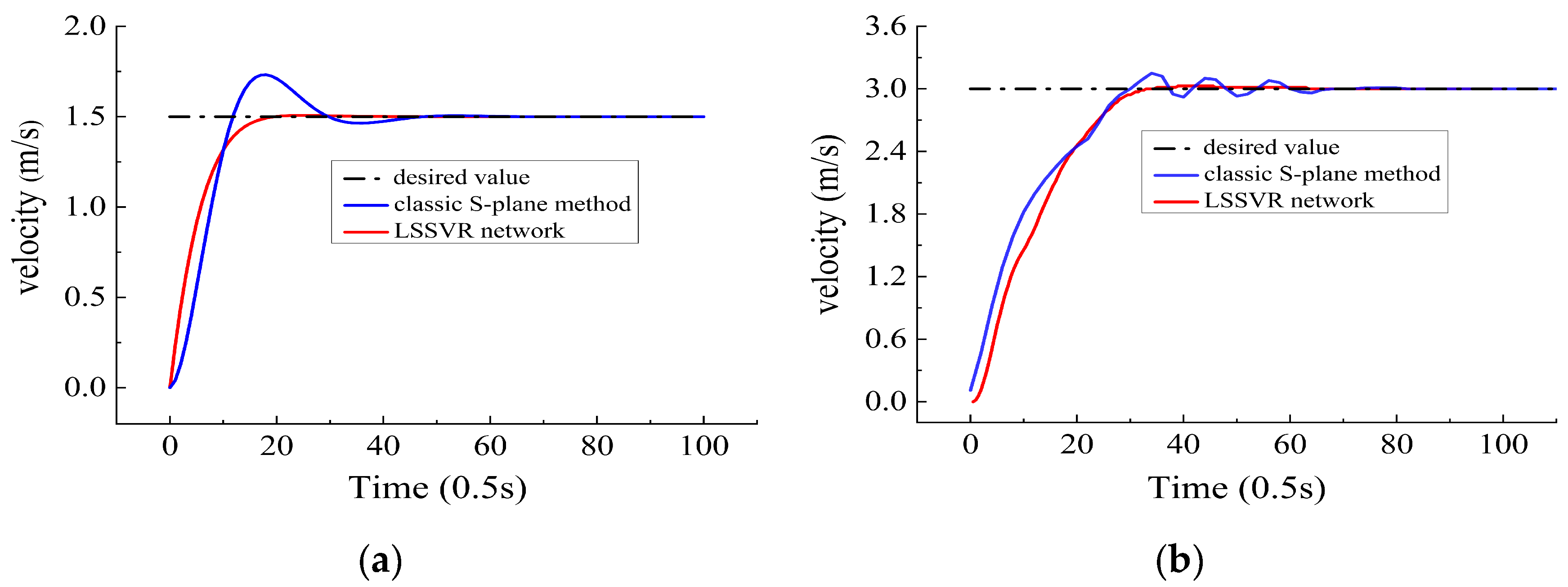
8.1. Contrast Trials on Velocity Control

In the velocity control trials based on the classic S-plane method and LSSVR network, the AUV was stationary at the water surface. With regard to the requirements on AUV engineering practice, the desired velocity was set to be 1.5 m/s in the horizontal plane. The control results based on the two different methods are shown in Figure 13a and Figure 14a, and the detailed data on the same scale unit ranging from 300 to 400 control beats during the control process are in Figure 13b and Figure 14b, respectively.

As shown in Figure 13a, the velocity control results based on classic S-plane method showed drastically frequent fluctuations and permissible overshoots. When put in a scale unit of 0.15 on the velocity axis, such deviations were more noticeable as shown in Figure 13b.

In Figure 14a, the system based on LSSVR interactive network presented better control results despite the frequent fluctuations as a result of the impact from the water currents during the sea trial. The system reached the stability state with a shorter time than that based on the classic S-plane method. Additionally, with the same scale unit in the detailed graph as shown in Figure 14b, the fluctuations and deviations were much milder than that caused by the classic S-plane method during the control period ranging from 300 to 400 beats.

8.2. Contrast Trials on Heading Control

In the heading control based on the classic S-plane method and LSSVR network, the AUV started with an initial heading angle of 120° and a desired heading angle of 90°. The trial results based on the two different methods are shown in Figure 15a and Figure 16a, respectively, and the detailed data in the same scale unit are in Figure 15b and Figure 16b, respectively.

As shown in Figure 15a, the heading control results based on classic S-plane method were subject to frequent and noticeable ups and downs around the desired value. Especially in the detailed results ranging from 300 to 400 control beats as shown in Figure 15b, the deviations were drastic with the maximum bias as high as 6° on the axis in a scale unit of 2 degrees.

In Figure 16a, in contrast, the system based on the LSSVR network was much more stable with subtle fluctuations. The smooth control curve well fitted the desired value. During the period ranging from 300 to 400 beats in Figure 16b, the curve almost stuck to the desired value with deviations of no more than 1°.

8.3. Analysis on Contrastive Trials

According to the control results of the sea trials with the classic S-plane method and the LSSVR network, evaluation indicators are introduced for comparison of the two control methods. The indicators include the maximum overshoot, standard deviation and arithmetic mean value. As shown in

Table 2. Evaluation indicators of control results based on two different methods.

	Velocity Control (1.5 m/s)		Heading Control (90°)
	Classic S-Plane	LSSVR Network	Classic S-Plane	LSSVR Network
maximum overshoot	0.150 m/s	0.057 m/s	6.097°	1.675°
standard deviation	0.087 m/s	0.023 m/s	1.233°	0.223°
arithmetic mean value	1.499 m/s	1.499 m/s	91.954°	90.186°

, the indicators and analysis focus on the control results ranging from the 300 to 400th control beats during the control period.

In the velocity control, the system based on the LSSVR network performed better with a smaller maximum overshoot and standard deviation. Moreover, the superiority and effectiveness of the LSSVR network can be seen in the heading control. Because of the water currents, the system based on the classic S-plane method suffered from violent fluctuations and showed a maximum overshoot of 6.097°. In contrast, the LSSVR network withstood the external disturbance, stabilizing the system with a standard deviation of 0.223° and an arithmetic mean value of 90.186°, which were considered of high accuracy in complex engineering contexts.

Based on the trial results, as a widely used method for AUV control, the classic S-plane method proved again its effectiveness with satisfactory performance in the sea trials, fully competent in ordinary underwater operations. The LSSVR network, however, exceeded the classic S-plane method in respect to the response time, convergence time and control accuracy due to its ability in precise identification of the dynamic characteristics, as well as offline design and online optimization of the control law of the research object. In this regard, the LSSVR network can be of practical use in underwater tasks, as it has high expectations on control precision.

8.4. Path Following

The path following was carried out near the water surface to verify the potential application of the LSSVR network in underwater pipeline search, scanning operations or multi-vehicle navigation. As shown in Figure 17, the desired path was designed intentionally to be non-orthogonal with the longitude or latitude, with five turning points to examine the effectiveness and robustness of the LSSVR network. The four line segments, namely AB–BC–CD–DE, were approximately 490 m, 160 m, 350 m and 100 m, respectively, with a desired control depth of 0.5 m under the surface. In general, the 5-time length of the AUV length is considered as the acceptable range for path following. Considering the influence of water currents and verification of the control accuracy of the network, the entry of the acceptable range with a radius of 9 m was recognized as the AUV’s success of reaching each turning point in practical engineering operations.

The desired route was approximately 1105 m. With a cruise velocity of 1 m/s, the AUV was expected to complete the following in about 2210 control beats. In view of the deviations between the actual position and the desired position in longitude, latitude and depth, Figure 18 showed the AUV’s following information on each segment route (namely routes AB, BC, CD and DE) together with their detailed data during the corresponding cruise time.

Despite the varying turbulence and surge, the effectiveness of the LSSVR network was verified by the trial results. The interactions between the online module and the offline module achieved the real-time optimization of the control law, enabling the AUV precise identification of the operation site and robustness against the external interference. It can be calculated based on Figure 18 and

Table 3. Analysis of path following based on LSSVR method.

Position	Maximum Deviation			Arithmetic Mean Value
	Longitude (m)	Latitude (m)	Depth (m)	Longitude (m)	Latitude (m)	Depth (m)
A–B (400–500 beat)	0.653	0.642	0.056	0.013	0.457	0.026
B–C (1070–1170 beat)	0.354	0.651	0.044	−0.268	0.131	0.022
C–D (1550–1650 beat)	0.499	0.465	0.041	0.141	0.145	0.020
D–E (2060–2160 beat)	0.596	0.637	0.046	0.261	0.163	0.019

that the LSSVR network managed to maintain the deviations in longitude and latitude within 0.7 m, with small depth deviations of no more than 0.05 m during the AUV’s route along each direct segment route. Such control precision was of practical use in engineering practices that have high requirements on control accuracy.

The heading control responses in the trial were shown in Figure 19. In Figure 19a, four steps were designed along the route at four turning points. As can be seen from the detailed heading data in Figure 19b, it took the AUV approximately 40 s to realize the heading change during the 800–1200 control beats. During the aforesaid period, the maximum overshoot was 2.7° with an arithmetic mean value of 0.38°. The practicability of the LSSVR network was also verified by the AUV’s entrance into the acceptable range of the five waypoints. As shown in Figure 20, the AUV approached the turning waypoints with adequate redundancy to the boundary of the 9 m acceptable circle. The path following results provided strong evidence that the LSSVR interactive network can be of practical application in formation navigation operations or search tasks.

8.5. Long-Range Cruise

The 12.5 km long route consisted of two pocket-shaped polygons (first half in blue and second half in red) as shown in Figure 21. The AUV completed the cruise in 3.5 h at an average speed of 1.0 m/s. During the trial, both the hardware and software structures of the AUV served well with no physical damage or failure. At the sharp turns in particular, the LSSVR network enabled the AUV to respond immediately to the control instructions. The cruise proved the stability and reliability of the LSSVR network in long-time and long-range operations.

9. Conclusions

A new motion control method based on LSSVR network structure is proposed in this study. The existing methods have generally met the requirements of engineering operations on the control accuracy, but some are still limited in practical use as the result of complicated structure or demanding parameter regulations. Moreover, many of the present methods are not able to satisfy the high expectations of tasks that have demanding requirements on the control accuracy. For this reason, an interactive structure composed of online module and offline module is designed based on the strong and efficient leaning ability of LSSVR. The reciprocal network structure aims to improve the control accuracy with the offline module responsible for the identification of the AUV’s kinematic characteristics and design of the control law, while the online module for real-time optimization of the control law based on the newly-learned knowledge on the working context.

In order to verify the effectiveness of the LSSVR network, contrastive simulation experiments under different conditions were conducted with the classic S-plane method, a widely used approach in AUV engineering. As the experiments results showed, the LSSVR interactive network achieved better performance in the velocity control and heading control with shorter time reaching the stability state and barely overshoots.

Following the simulation experiments, sea trials were carried out to further examine the LSSVR network. Since motion control is the foundation for all functions, contrastive trials with the classic S-plane method on velocity control and heading control were first conducted. The LSSVR network excelled in the classic S-plane method, with a maximum overshoot of 0.057 m/s and a standard deviation of 0.023 m/s in the velocity control, as well as a maximum overshoot of 1.675° and a standard deviation of 0.223° in the heading control. Then, on the basis of motion control accuracy, the path following trial proceeded to verify the effectiveness of the LSSVR network in underwater operations including pipeline detection, multi-vehicle formation navigation or pectinate search. The LSSVR network enabled the AUV to follow the desired route with deviations of no more than 0.7 m in longitude and latitude as well as precision in depth following, with a deviation of no more than 0.06 m. Additionally, the AUV approached the turning points on the route by entering the 9 m acceptable range. Finally, a 3.5 h long-range cruise proved the stability and reliability of the LSSVR interactive network under changing water currents, especially when little knowledge on the operation site is available.

The research object in this study is driven by the propeller–rudder system, but theoretically the research findings are also of reference meaning to thruster-driven AUVs. Subsequent studies will concentrate on the effectiveness of the LSSVR interactive network on AUVs of different propulsion systems and dimensions. In addition, future studies will also focus on simplicity of the proposed network to improve its practicability.

References

1. Alhaddad, S.; Förstner, J.; Grynko, Y. Numerical study of light backscattering from layers of absorbing irregular particles larger than the wavelength. J. Quant. Spectrosc. Radiat. Transf. 2023, 302, 108557. [Google Scholar] [CrossRef]
2. Monebi, A.M.; Otgonbat, D.; Ahn, B.C.; Lee, C.S.; Ahn, J.H. Conceptual Design of a Semi-Dual Polarized Monopulse Antenna by Computer Simulation. Appl. Sci. 2023, 13, 2960. [Google Scholar] [CrossRef]
3. Rutkowska, D.; Duda, P.; Cao, J.; Rutkowski, L.; Byrski, A.; Jaworski, M.; Tao, D. The L2 convergence of stream data mining algorithms based on probabilistic neural networks. Inf. Sci. 2023, 631, 346–368. [Google Scholar] [CrossRef]
4. Kannan, R.; Nandwana, P. Accelerated alloy discovery using synthetic data generation and data mining. Scr. Mater. 2023, 228, 115335. [Google Scholar] [CrossRef]
5. Wadi, A.; Mukhopadhyay, S. A novel localization-free approach to system identification for underwater vehicles using a Universal Adaptive Stabilizer. Ocean Eng. 2023, 274, 114013. [Google Scholar] [CrossRef]
6. Baidillah, M.R.; Busono, P.; Riyanto, R. Mechanical ventilation intervention based on machine learning from vital signs monitoring: A scoping review. Meas. Sci. Technol. 2023, 34, 2001. [Google Scholar] [CrossRef]
7. Pena, A.; Tejada, J.C.; Gonzalez-Ruiz, J.D.; Sepúlveda-Cano, L.M.; Chiclana, F.; Caraffini, F.; Gongora, M. An evolutionary intelligent control system for a flexible joints robot. Appl. Soft Comput. J. 2023, 135, 110043. [Google Scholar] [CrossRef]
8. Perera, Y.S.; Ratnaweera, D.A.A.C.; Dasanayaka, C.H.; Abeykoon, C. The role of artificial intelligence-driven soft sensors in advanced sustainable process industries: A critical review. Eng. Appl. Artif. Intell. 2023, 121, 105988. [Google Scholar] [CrossRef]
9. Bigman, D.P.; Day, D.J. Ground penetrating radar inspection of a large concrete spillway: A case-study using SFCW GPR at a hydroelectric dam. Case Stud. Constr. Mater. 2022, 16, e000975. [Google Scholar] [CrossRef]
10. Character, L.; Ortiz, A., Jr.; Beach, T.; Luzzadder-Beach, S. Archaeologic Machine Learning for Shipwreck Detection Using Lidar and Sonar. Remote Sens. 2021, 13, 1759. [Google Scholar] [CrossRef]
11. Wang, W.; Gao, Y. Pipeline leak detection method based on acoustic-pressure information fusion. Measurement 2023, 212, 112691. [Google Scholar] [CrossRef]
12. Arif, J.; Rehman-Shaikh, M.A.; Evangelou, S.A. Novel evaluation and testing of technology qualification process of subsea oil and gas products. J. Pet. Sci. Eng. 2022, 208, 109576. [Google Scholar] [CrossRef]
13. Toro, N.; Galvez, E.; Saldana, M.; Jeldres, R.I. Submarine mineral resources: A potential solution to political conflicts and global warming. Miner. Eng. 2022, 179, 107441. [Google Scholar] [CrossRef]
14. Lu, J.; Feng, W.; Li, Y.; Zhang, J.; Zou, Y.; Li, J. VMD and self-attention mechanism-based Bi-LSTM model for fault detection of optical fiber composite submarine cables. EURASIP J. Adv. Signal Process. 2023, 2023, 000988. [Google Scholar] [CrossRef]
15. Misiuk, B.; Lecours, V.; Dolan, M.F.J.; Robert, K. Evaluating the Suitability of Multi-Scale Terrain Attribute Calculation Approaches for Seabed Mapping Applications. Mar. Geod. 2021, 44, 327–385. [Google Scholar] [CrossRef]
16. Khutornaia, E.; Gnevashev, Y. Development of an Application for Controlling an Underwater Vehicle. Transp. Res. Procedia 2023, 68, 858–862. [Google Scholar] [CrossRef]
17. Tholen, C.; El-Mihoub, T.A.; Nolle, L.; Zielinski, O. Artificial Intelligence Search Strategies for Autonomous Underwater Vehicles Applied for Submarine Groundwater Discharge Site Investigation. J. Mar. Sci. Eng. 2021, 10, 7. [Google Scholar] [CrossRef]
18. Madanipour, V.; Najafi, F. Modal analysis of underwater hull cleaning robot considering environmental interaction. Ocean Eng. 2023, 273, 113821. [Google Scholar] [CrossRef]
19. Kolesnikov, A.A.; Yakimenko, O.I.; Radionov, I.A.; Kaliy, D.S. Comparison of the Methods of Classical and Synergetic Theories of Control of the Movement Autonomous Underwater Machine. Mekhatronika Avtom. Upr. 2019, 20, 663–668. [Google Scholar] [CrossRef]
20. Ahn, J.K.; Koh, G.; So, M.O. Nonlinear PD Depth Control for Autonomous Underwater Vehicle. J. Fishries Mar. Sci. Educ. 2019, 31, 949–959. [Google Scholar]
21. Bingul, Z.; Gul, K. Intelligent-PID with PD Feedforward Trajectory Tracking Control of an Autonomous Underwater Vehicle. Machines 2023, 11, 300. [Google Scholar] [CrossRef]
22. Zhilenkov, A.; Chernyi, S.; Firsov, A. Autonomous Underwater Robot Fuzzy Motion Control System with Parametric Uncertainties. Designs 2021, 5, 24. [Google Scholar] [CrossRef]
23. Duan, K.; Fong, S.; Chen, C.P. Fuzzy observer-based tracking control of an underactuated underwater vehicle with linear velocity estimation. IET Control. Theory Appl. 2020, 14, 584–593. [Google Scholar] [CrossRef]
24. Guerrero, J.; Chemori, A.; Torres, J.; Creuze, V. Time-delay high-order sliding mode control for trajectory tracking of autonomous underwater vehicles under disturbances. Ocean Eng. 2023, 268, 113375. [Google Scholar] [CrossRef]
25. Vadapalli, S.; Mahapatra, S. 3D Path Following Control of an Autonomous Underwater Robotic Vehicle Using Backstepping Approach Based Robust State Feedback Optimal Control Law. J. Mar. Sci. Eng. 2023, 11, 277. [Google Scholar] [CrossRef]
26. Chen, H.; Tang, G.; Wang, S.; Guo, W.; Huang, H. Adaptive fixed-time backstepping control for three-dimensional trajectory tracking of underactuated autonomous underwater vehicles. Ocean Eng. 2023, 275, 114109. [Google Scholar] [CrossRef]
27. Wen, L.; Yu, S.; Zhao, Y.; Yan, Y. Adaptive dynamic event-triggered consensus control of multiple autonomous underwater vehicles. Int. J. Control 2023, 96, 746–756. [Google Scholar] [CrossRef]
28. Hasan, M.W.; Abbas, N.H. Disturbance Rejection for Underwater robotic vehicle based on adaptive fuzzy with nonlinear PID controller. ISA Trans. 2022, 130, 360–376. [Google Scholar] [CrossRef]
29. Yan, Z.; Yang, H.; Zhang, W.; Gong, Q.; Zhang, Y.; Zhao, L. Robust nonlinear model predictive control of a bionic underwater robot with external disturbances. Ocean Eng. 2022, 253, 111310. [Google Scholar] [CrossRef]
30. Khoshnam, S. Neural network feedback linearization target tracking control of underactuated autonomous underwater vehicles with a guaranteed performance. Ocean Eng. 2022, 258, 111827. [Google Scholar]
31. Muñoz, F.; Cervantes-Rojas, J.S.; Valdovinos, J.M.; Sandre-Hernández, O.; Salazar, S.; Romero, H. Dynamic Neural Network-Based Adaptive Tracking Control for an Autonomous Underwater Vehicle Subject to Modeling and Parametric Uncertainties. Appl. Sci. 2021, 11, 2797. [Google Scholar] [CrossRef]
32. Mazare, M.; Asharioun, H.; Davoudi, E.; Mokhtari, M. Distributed finite-time neural network observer-based consensus tracking control of heterogeneous underwater vehicles. Ocean Eng. 2023, 272, 113882. [Google Scholar] [CrossRef]
33. Elhaki, O.; Shojaei, K.; Mehrmohammadi, P. Reinforcement learning-based saturated adaptive robust neural-network control of underactuated autonomous underwater vehicles. Expert Syst. Appl. 2022, 197, 116714. [Google Scholar] [CrossRef]
34. Qin, H.; Si, J.; Wang, N.; Gao, L.; Shao, K. Disturbance Estimator-Based Nonsingular Fast Fuzzy Terminal Sliding-Mode Formation Control of Autonomous Underwater Vehicles. Int. J. Fuzzy Syst. 2023, 25, 395–406. [Google Scholar] [CrossRef]
35. Menezes, J.; Sands, T. Discerning Discretization for Unmanned Underwater Vehicles DC Motor Control. J. Mar. Sci. Eng. 2023, 11, 436. [Google Scholar] [CrossRef]
36. Sedghi, F.; Arefi, M.M.; Abooee, A. Command filtered-based neuro-adaptive robust finite-time trajectory tracking control of autonomous underwater vehicles under stochastic perturbations. Neurocomputing 2023, 519, 158–172. [Google Scholar] [CrossRef]
37. Jiang, C.; Lv, J.; Wan, L.; Wang, J.; He, B.; Wu, G. An Improved S-Plane Controller for High-Speed Multi-Purpose AUVs with Situational Static Loads. J. Mar. Sci. Eng. 2023, 11, 646. [Google Scholar] [CrossRef]
38. He, Y.; Xie, Y.; Pan, G.; Cao, Y.; Huang, Q.; Ma, S.; Zhang, D.; Cao, Y. Depth and Heading Control of a Manta Robot Based on S-Plane Control. J. Mar. Sci. Eng. 2022, 10, 1698. [Google Scholar] [CrossRef]
39. Shankar, D.D.; Azhakath, A.S. Random embedded calibrated statistical blind steganalysis using cross validated support vector machine and support vector machine with particle swarm optimization. Sci. Rep. 2023, 13, 2359. [Google Scholar] [CrossRef]
40. Rahimkhani, P.; Ordokhani, Y. Chelyshkov least squares support vector regression for nonlinear stochastic differential equations by variable fractional Brownian motion. Chaos Solitons Fractals Interdiscip. J. Nonlinear Sci. Nonequilib. Complex Phenom. 2022, 163, 112570. [Google Scholar] [CrossRef]
41. Abdollahzadeh, M.; Khosravi, M.; Hajipour Khire Masjidi, B.; Samimi Behbahan, A.; Bagherzadeh, A.; Shahkar, A.; Tat Shahdost, F. Estimating the density of deep eutectic solvents applying supervised machine learning techniques. Sci. Rep. 2022, 12, 4954. [Google Scholar] [CrossRef] [PubMed]
42. Pakniyat, A.; Parand, K.; Jani, M. Least squares support vector regression for differential equations on unbounded domains. Chaos Solitons Fractals Interdiscip. J. Nonlinear Sci. Nonequilib. Complex Phenom. 2021, 151, 111232. [Google Scholar] [CrossRef]
43. Zhang, B.; Ji, D.; Liu, S.; Zhu, X.; Xu, W. Autonomous Underwater Vehicle navigation: A review. Ocean Eng. 2023, 273, 113861. [Google Scholar] [CrossRef]
44. Cenerini, J.; Mehrez, M.W.; Han, J.W.; Jeon, S.; Melek, W. Model Predictive Path Following Control without terminal constraints for holonomic mobile robots. Control Eng. Pract. 2023, 132, 105406. [Google Scholar] [CrossRef]
45. Krejčí, J.; Babiuch, M.; Babjak, J.; Suder, J.; Wierbica, R. Implementation of an Embedded System into the Internet of Robotic Things. Micromachines 2022, 14, 113. [Google Scholar] [CrossRef] [PubMed]
46. Christensen, L.; de Gea Fernández, J.; Hildebrandt, M.; Koch, C.E.S.; Wehbe, B. Recent Advances in AI for Navigation and Control of Underwater Robots. Curr. Robot. Rep. 2022, 3, 165–175. [Google Scholar] [CrossRef]
47. Machlev, R.; Perl, M.; Caciularu, A.; Belikov, J.; Levy, K.Y.; Levron, Y. Explaining the decisions of power quality disturbance classifiers using latent space features. Int. J. Electr. Power Energy Syst. 2023, 148, 108949. [Google Scholar] [CrossRef]
48. Palar, P.S.; Parussini, L.; Bregant, L.; Shimoyama, K.; Zuhal, L.R. On kernel functions for bi-fidelity Gaussian process regressions. Struct. Multidiscip. Optim. 2023, 66, 3487. [Google Scholar] [CrossRef]
49. Maroli, J.M. Generating discrete dynamical system equations from input–output data using neural network identification models. Reliab. Eng. Syst. Saf. 2023, 235, 109198. [Google Scholar] [CrossRef]
50. Weigand, J.; Deflorian, M.; Ruskowski, M. Input-to-state stability for system identification with continuous-time Runge–Kutta neural networks. Int. J. Control 2023, 96, 24–40. [Google Scholar] [CrossRef]
51. Parand, K.; Hasani, M.; Jani, M.; Yari, H. Numerical simulation of Volterra–Fredholm integral equations using least squares support vector regression. Comput. Appl. Math. 2021, 40, 246. [Google Scholar] [CrossRef]
52. Moqaddasi Amiri, M.; Tapak, L.; Faradmal, J. A mixed-effects least square support vector regression model for three-level count data. J. Stat. Comput. Simul. 2019, 89, 2801–2812. [Google Scholar] [CrossRef]
53. Daskin, A.; Gupta, R.; Kais, S. Dimension Reduction and Redundancy Removal through Successive Schmidt Decompositions. Appl. Sci. 2023, 13, 3172. [Google Scholar] [CrossRef]
54. Oh, K.S.; Lee, J.W. Auxiliary algorithm to approach a near-global optimum of a multi-objective function in acoustical topology optimization. Eng. Appl. Artif. Intell. 2023, 117, 105488. [Google Scholar] [CrossRef]
55. Shakeel, M.; Samanova, A.; Pourafshary, P.; Hashmet, M.R. Optimization of Low Salinity Water/Surfactant Flooding Design for Oil-Wet Carbonate Reservoirs by Introducing a Negative Salinity Gradient. Energies 2022, 15, 9400. [Google Scholar] [CrossRef]
Figure 1. Vertical view and lateral view of the AUV platform.
Jmse 11 01111 g001
Figure 2. Propeller, horizontal and vertical rudders.
Jmse 11 01111 g002
Figure 3. LSSVR interactive network.
Jmse 11 01111 g003
Figure 4. Sample data. (a) Samples of thrust voltage; (b) samples of velocity in surge direction; (c) samples of helm angle; (d) samples of heading angle.
Jmse 11 01111 g004
Figure 5. Identification result and deviation from velocity evaluation samples. (a) Identification results of velocity evaluation samples; (b) deviations from evaluation samples.
Jmse 11 01111 g005
Figure 6. Identification result and deviation from heading evaluation samples. (a) Identification results of heading evaluation samples; (b) deviations from evaluation samples.
Jmse 11 01111 g006
Figure 7. LSSVR control unit.
Jmse 11 01111 g007
Figure 8. Offline design of LSSVR controller.
Jmse 11 01111 g008
Figure 9. Online optimization of LSSVR controller.
Jmse 11 01111 g009
Figure 10. Contrast of velocity control results with classic S-plane method and LSSVR network. (a) Control result of velocity (1.5 m/s); (b) control result of velocity (3.0 m/s).
Jmse 11 01111 g010
Figure 11. Contrast of heading control results with classic S-plane method and LSSVR network. (a) Control results of heading (45°); (b) control results of heading (60°).
Jmse 11 01111 g011
Figure 12. The site and water current conditions of the sea trials. (a) The AUV in the sea trial; (b) the sea trial site; (c) water current conditions of the sea trial site.
Jmse 11 01111 g012
Figure 13. Results of velocity control based on classic S-plane method. (a) Control result of velocity; (b) deviations of control result ranging from 300 to 400 beats.
Jmse 11 01111 g013
Figure 14. Results of velocity control based on LSSVR network. (a) Control result of velocity; (b) details of control result ranging from 300 to 400 beats.
Jmse 11 01111 g014
Figure 15. Results of heading control based on classic S-plane method. (a) Control result of heading; (b) details of control result ranging from 300 to 400 beats.
Jmse 11 01111 g015
Figure 16. Results of heading control based on LSSVR network. (a) Control result of heading; (b) details of control result ranging from 300 to 400 beats.
Jmse 11 01111 g016
Figure 17. The trajectory of path following. (a) Trajectory in three-dimension view; (b) trajectory in plane view.
Jmse 11 01111 g017
Figure 18. Following deviations and local data. (a) Trajectory deviations from 1 to 980 control beats; (b) detailed trajectory deviations from 400 to 500 control beats; (c) trajectory deviations from 981 to 1300 control beats; (d) detailed trajectory deviations from 1070 to 1170 control beats; (e) trajectory deviations from 1301 to 2010 control beats; (f) detailed trajectory deviations from 1550 to 1650 control beats; (g) trajectory deviations from 2011 to 2200 control beats; (h) detailed trajectory deviations from 2060 to 2160 control beats.
Jmse 11 01111 g018aJmse 11 01111 g018b
Figure 19. Heading control responses and deviations. (a) Heading control data; (b) deviations between the desired and actual heading angles.
Jmse 11 01111 g019
Figure 20. AUV reaching of the waypoints. (a) Magnified view of reaching Point A; (b) magnified view of reaching Point B; (c) magnified view of reaching Point C; (d) magnified view of reaching Point D; (e) magnified view of reaching Point E.
Jmse 11 01111 g020aJmse 11 01111 g020b
Figure 21. Results of the long-range cruise.
Jmse 11 01111 g021