
Greenhouse Gas Emissions from Decommissioning Manmade Structures in the Marine Environment; Current Trends and Implications for the Future

Abstract
:1. Introduction
2. Materials and Methods
2.1. Methods
- The total estimate of costs to decommission everything in the North Sea was found (~£45 b over 20 years [6]).
- Then a percentage of this total was allocated to steel jackets, which make up 20% of the total [7].
- The total number of jackets was found, then the GHG emissions figure from [4] was applied. This represents 20% of the total infrastructure, so it was straightforward to determine the total GHG emissions.
- The total GHG emissions figure of 176 MtCO2e was divided by costs (~£45 b) to find the amount of GHG emissions figure per billion £ (3.83 MtCO2e/£b).
- The next stage was to find the cost of global decommissioning and apply the GHG figure/£b as determined in step 4.
- Future decommissioning trends were included, and a future GHG emission trend was determined.
- Decommissioning cost was established to be £1.333 b/GW [8].
- The GHG emissions per GW were determined to be 6.27 MtCO2e/GW [10].
- As the above figure does not include onshore activity such as dismantling, or onward transport, 20% was applied to the figure in step 2; 7.52 MtCO2e/GW
- Current wind capacity was then found; 55,678 MW for 2021 [13].
- The total GHG emissions from decommissioning were then found by multiplying capacity by GHG emissions; GHG emissions per GW x Capacity (GW) = Total GHG Emissions
2.2. Materials

| Offshore Hydrocarbon Decommissioning | |||
|---|---|---|---|
| Data | Unit | Reference | |
| UKNS number of steel structures | 320 | [6] | |
| Proportion of above to rest of infrastructure | 20 | % | |
| GHG emission per steel jacket | 110,000 | tCO2e | [4] |
| GHG to decom all steel jackets | 35.2 | MtCO2e | |
| Total GHG emissions | 176 | MtCO2e | |
| Total Cost | 45 | £b | [7] |
| GHG Emission per cost | 3.91 | MtCO2e/£b | |
| Onshore and shipping est | 20 | % | |
| Total GHG Emission per cost | 4.69 | MtCO2e/£b | |
| Global decom cost to 2024 | 42 | £b | [14] |
| Global decom GHG emissions to 2024 | 197.12 | MtCO2e/£b | |
| Rate of Decom growth | 4.9 | % | [14] |
| Offshore Wind Decommissioning | |||
|---|---|---|---|
| Input variables | Data | Unit | Reference |
| Decommissioning cost | 1.333 | £b/GW | [15] |
| GHG emissions per GW | 6.27 | MtCO2e | [10] |
| Onshore and shipping estimate | 20 | % | |
| Decommissioning emissions | 7.52 | MtCO2e/GW | |
| Wind capacity 2021 | 55,678 | MW | [13] |
| Growth rate from previous year | 62 | % | [11] |
| Growth rate 2019–2024 | 18.6 | % | [11] |
| Growth rate from 2024 | 8.20 | % | [10] |
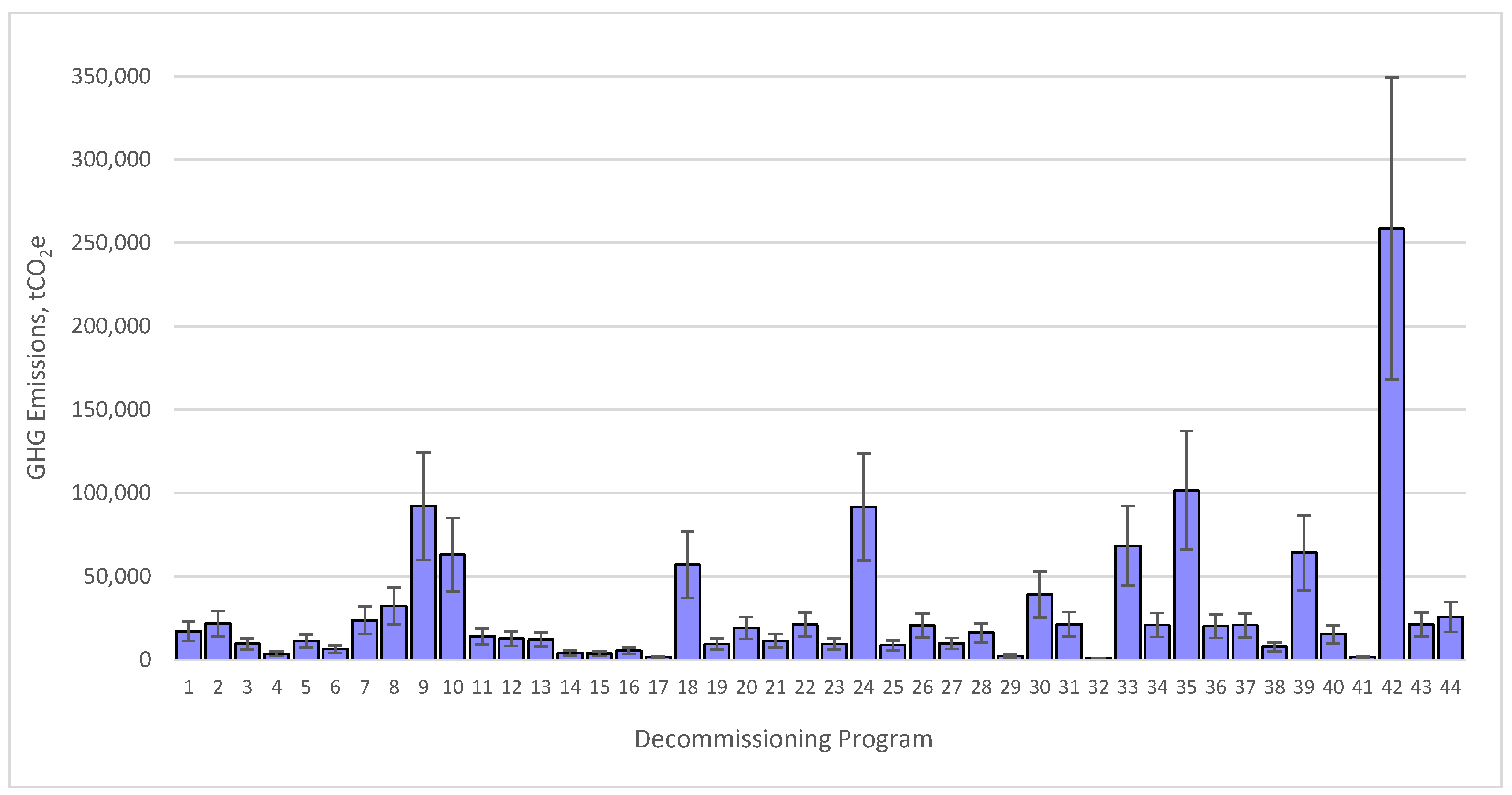
| GHG Emissions from North Sea OGI Decommissioning Programs | ||||
|---|---|---|---|---|
| Name | Operator | GHG Emissions (tCO2e) | No. On Graph | Reference |
| North Cormorant Topsides | TAQA | 17,018 | 1 | [16] |
| Tern Topsides | TAQA | 21,667 | 2 | [17] |
| PL301 Heimdal to Brae Alpha Condensate Pipeline | Equinor | 9,487 | 3 | [18] |
| Gaupe | Shell | 3,506 | 4 | [19] |
| Buchan & Hannay | Repsol Sinopec | 11,232 | 5 | [20] |
| Ensign | Spirit Energy | 6,344 | 6 | [21] |
| Windermere | INEOS | 23,574 | 7 | [22] |
| East Brae and Braemar | Marathon Oil | 32,191 | 8 | [23] |
| Brae Alpha | Marathon Oil | 92,000 | 9 | [24] |
| Brent | Shell | 63,045 | 10 | [25] |
| Atlantic & Cromarty | Hess Ltd. & BG group | 14,000 | 11 | [26] |
| Anglia | Ithaca Energy | 12,600 | 12 | [27] |
| Alma & Galica | EnQuest | 11,952 | 13 | [28] |
| Brynhild | Lunin | 3,998 | 14 | [29] |
| Cavendish | Ineos | 3,686 | 15 | [30] |
| Caister | Chrysaor | 5,374 | 16 | [31] |
| Cormorant Alpha Derrick | TAQA | 1,639 | 17 | [32] |
| South Morecambe DP3-DP4 | Spirit Energy | 56,876 | 18 | [33] |
| Eider Topsides | TAQA | 9,411 | 19 | [34] |
| LOGGS Area | Chrysaor | 19,019 | 20 | [35] |
| Macculloch | ConocoPhillips | 11,262 | 21 | [36] |
| Ketch and Schooner | DNO | 21,018 | 22 | [37] |
| Juliet | Neptune Energy | 9,388 | 23 | [38] |
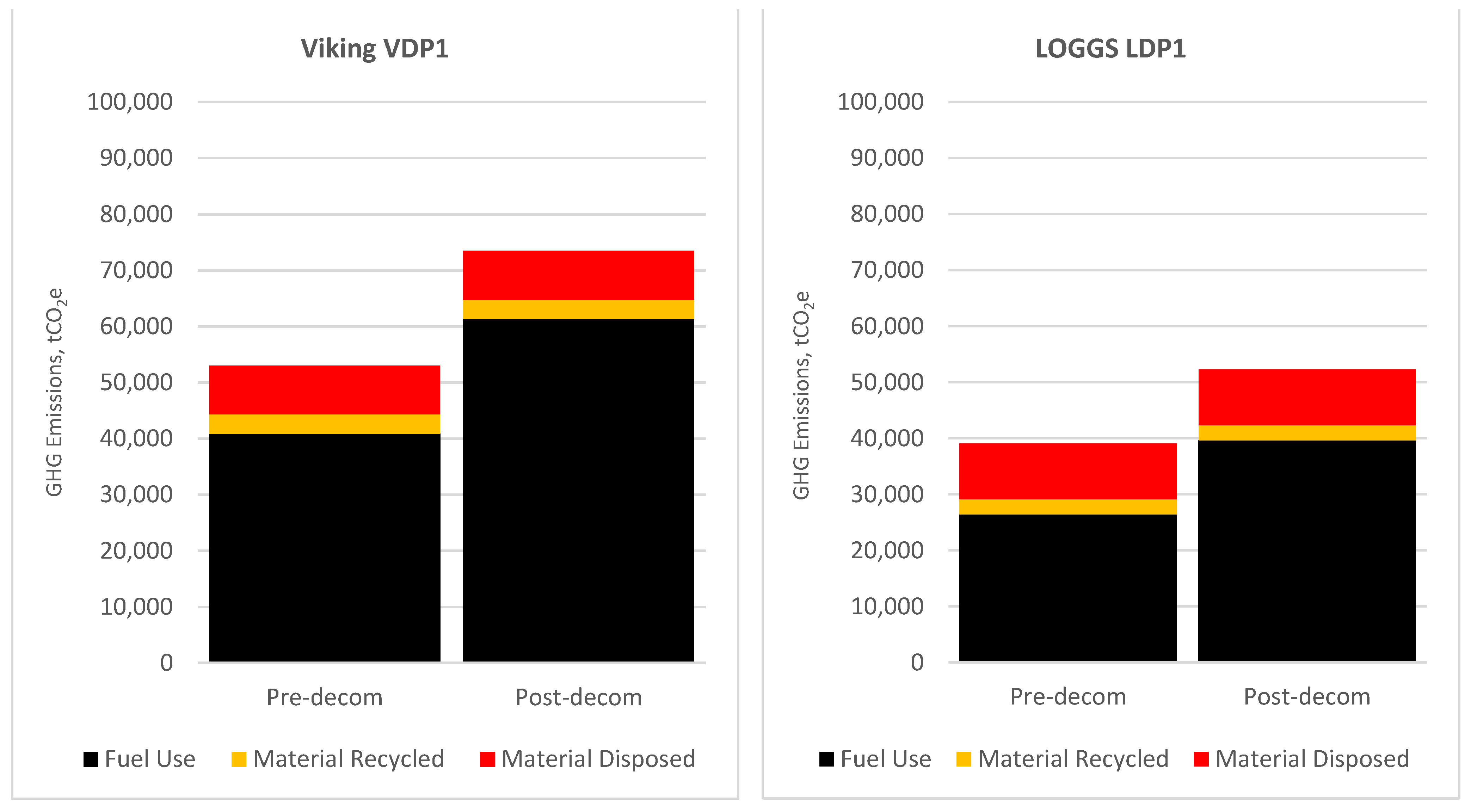
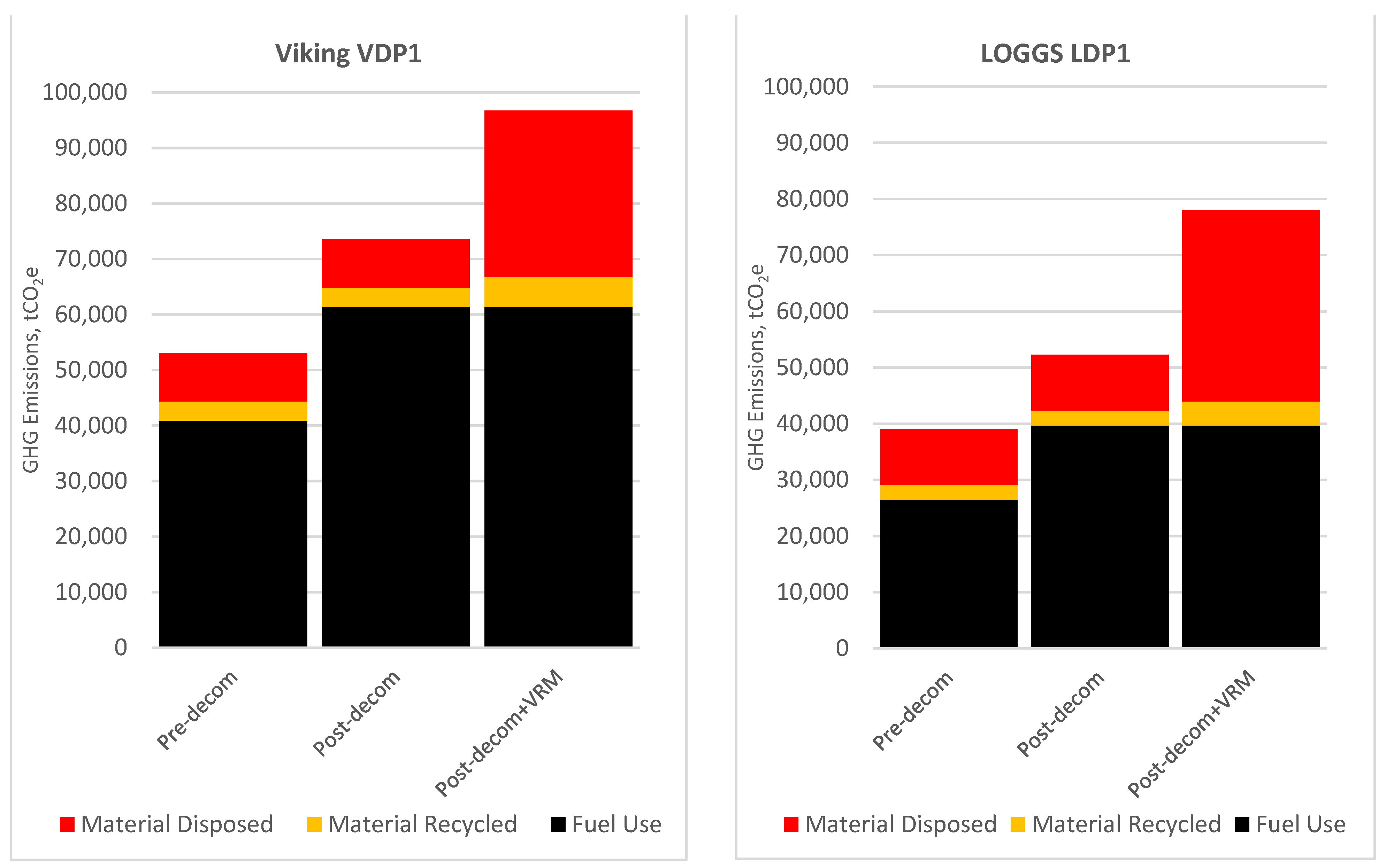
| Viking VDP1 and Loggs LDP1 | ConocoPhillips | 91,623 | 24 | [39] |
| Merlin | Fairfield | 8,619 | 25 | [40] |
| Ospey | Fairfield | 20,579 | 26 | [41] |
| Dunlin | Fairfield | 9,704 | 27 | [42] |
| Markham | Spirit Energy | 16,280 | 28 | [43] |
| Rev | Repsol | 2,421 | 29 | [44] |
| Saturn (Annabel) & Audrey Fields | Spirit Energy | 39,227 | 30 | [45] |
| Ann & Alison Fields | Spirit Energy | 21,250 | 31 | [46] |
| Ann A4 | Centrica | 745 | 32 | [47] |
| Etrick & Blackbird | Nexen | 68,263 | 33 | [48] |
| Athena Field | Ithaca Energy | 20,717 | 34 | [49] |
| Janice, James, Affleck Fields | Maersk Oil | 101,507 | 35 | [50] |
| Tyne | Perenco | 20,143 | 36 | [51] |
| Guinevee | Perenco | 20,668 | 37 | [52] |
| Leadon | Maersk Oil | 7,740 | 38 | [53] |
| Curlew | Shell | 64,200 | 39 | [54] |
| Jacky | Ithaca Energy | 15,177 | 40 | [55] |
| Bains | Spirit Energy | 1,673 | 41 | [56] |
| VDP2 | ConocoPhillips | 258,549 | 42 | [57] |
| VDP3 | ConocoPhillips | 20,980 | 43 | [57] |
| Rubie Renee | Endeavor | 25,627 | 44 | [58] |
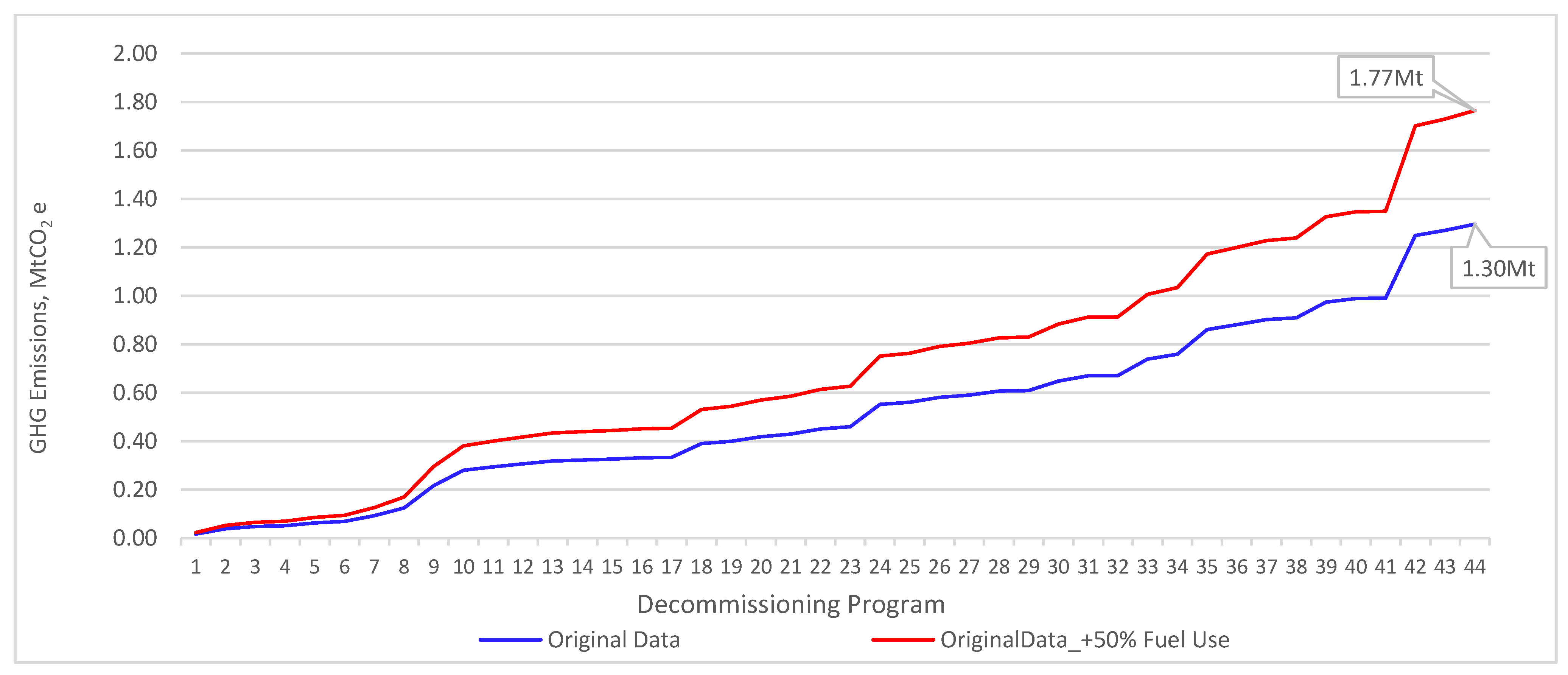
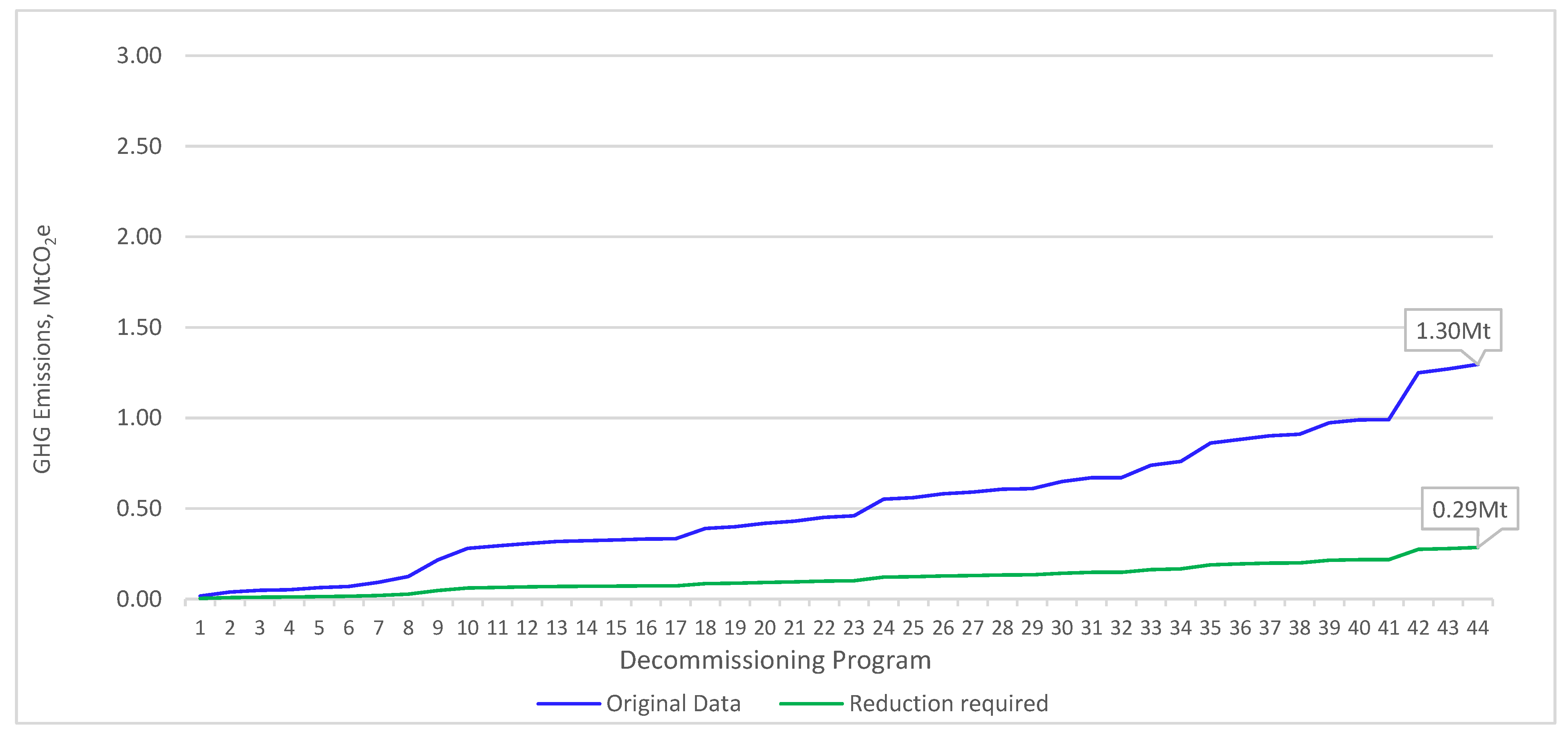
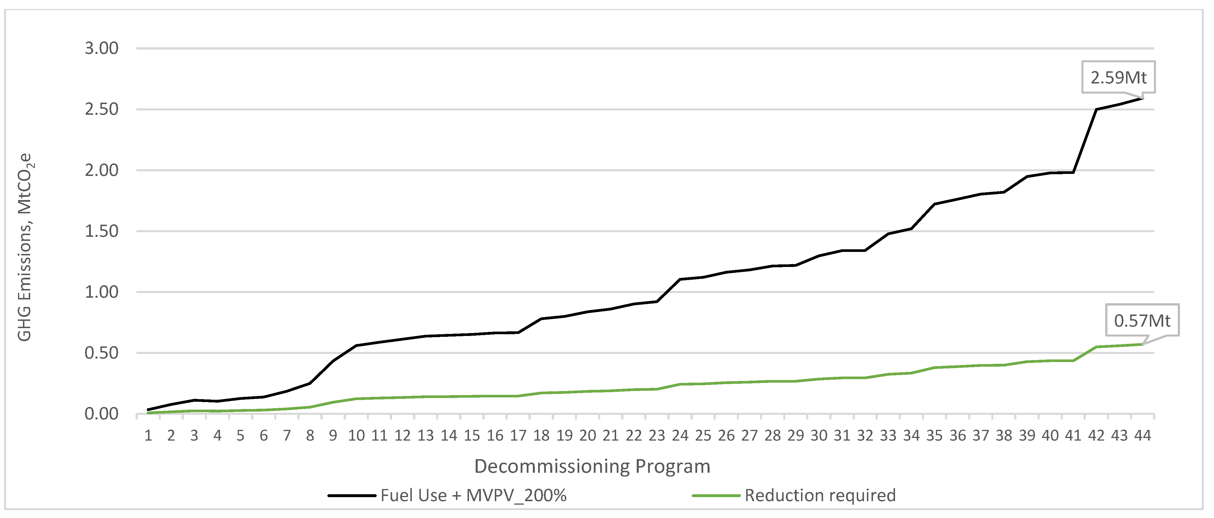
| Cumulative Emissions (tCO2e) | 1,295,978 | |||
3. Results
3.1. Reported Pre-Decommissioning GHG Emissions
3.2. Close-Out Report GHG Emissions
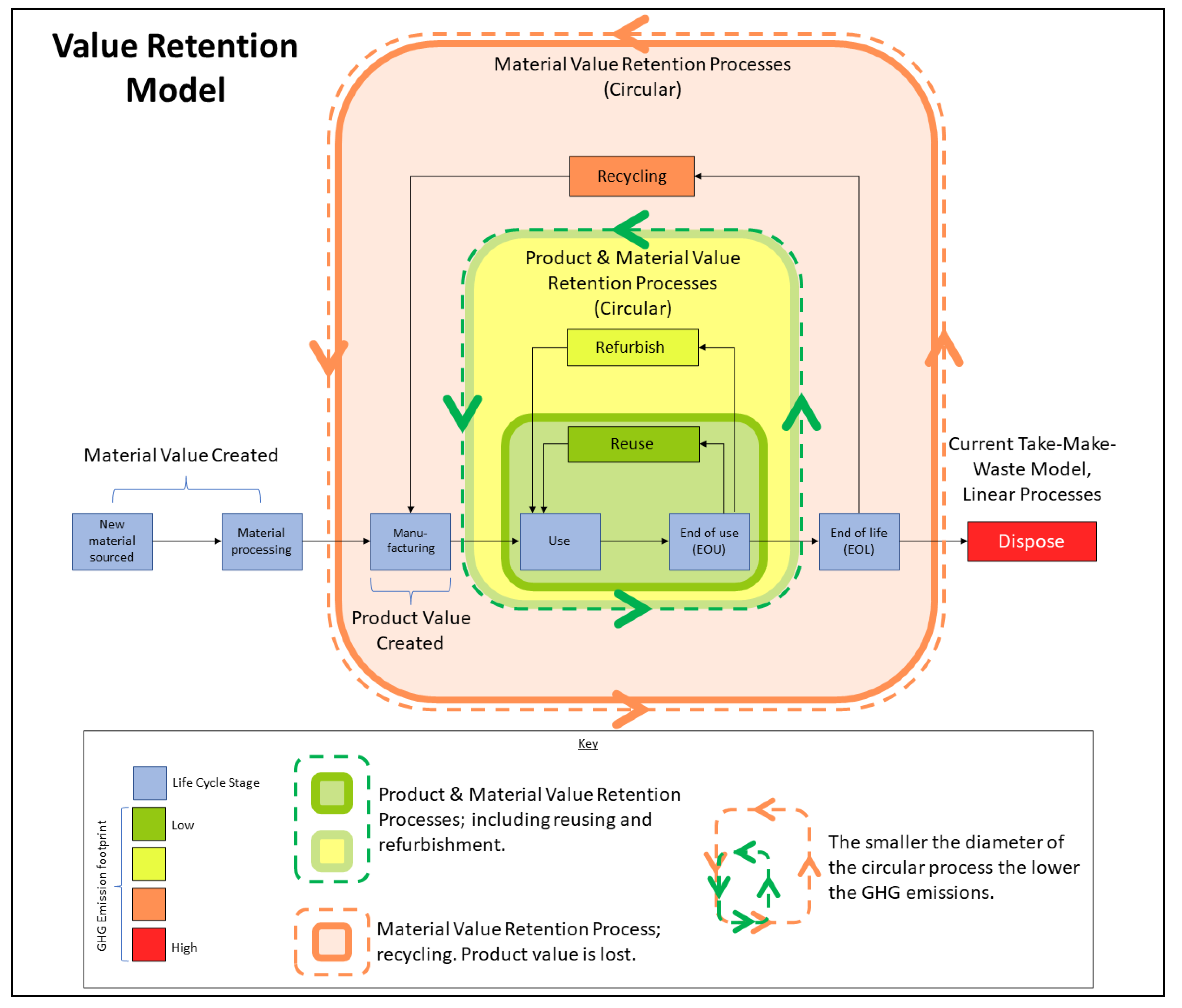
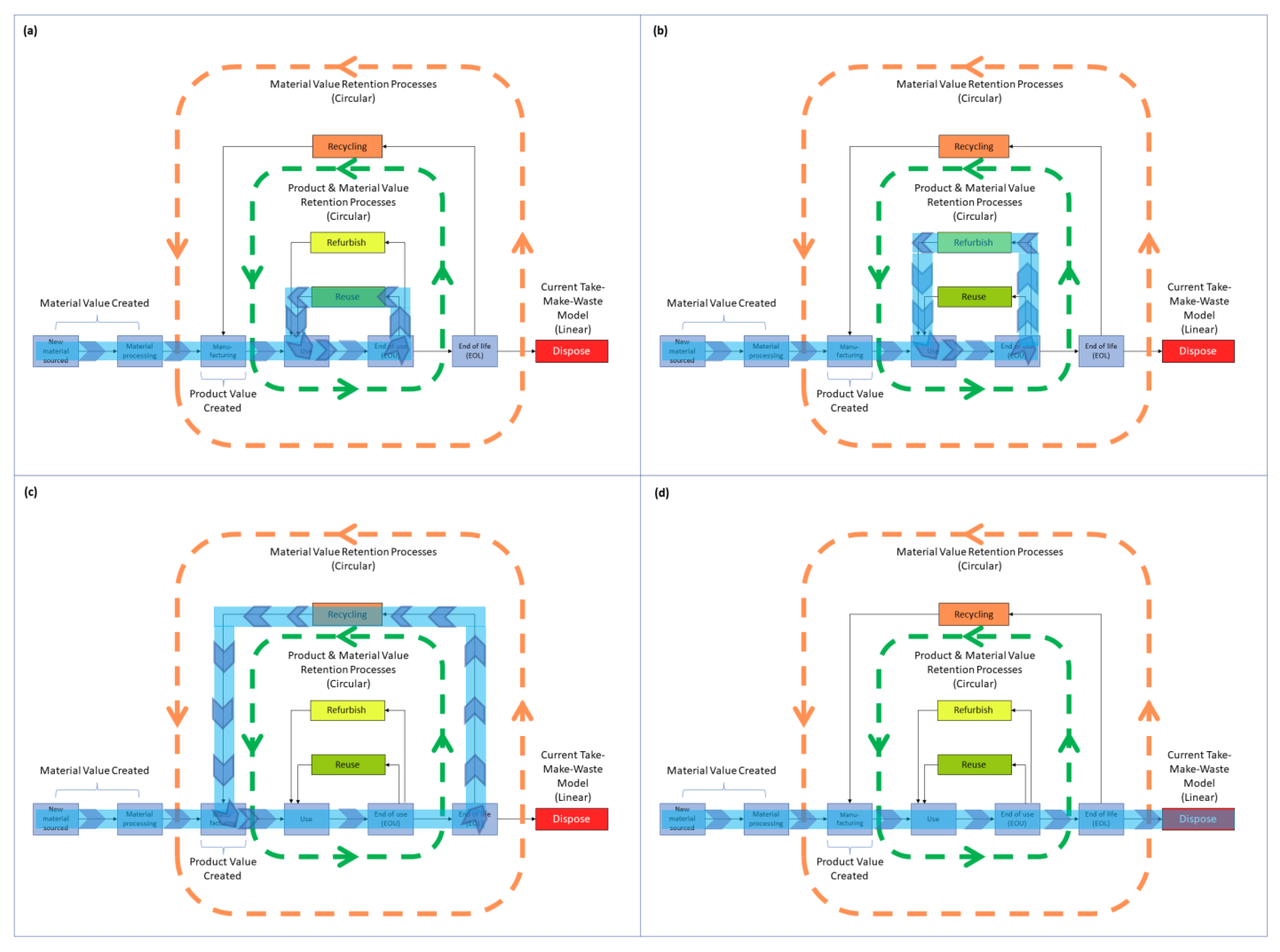
3.3. Value Retention Model GHG Emissions
3.4. Decarbonization
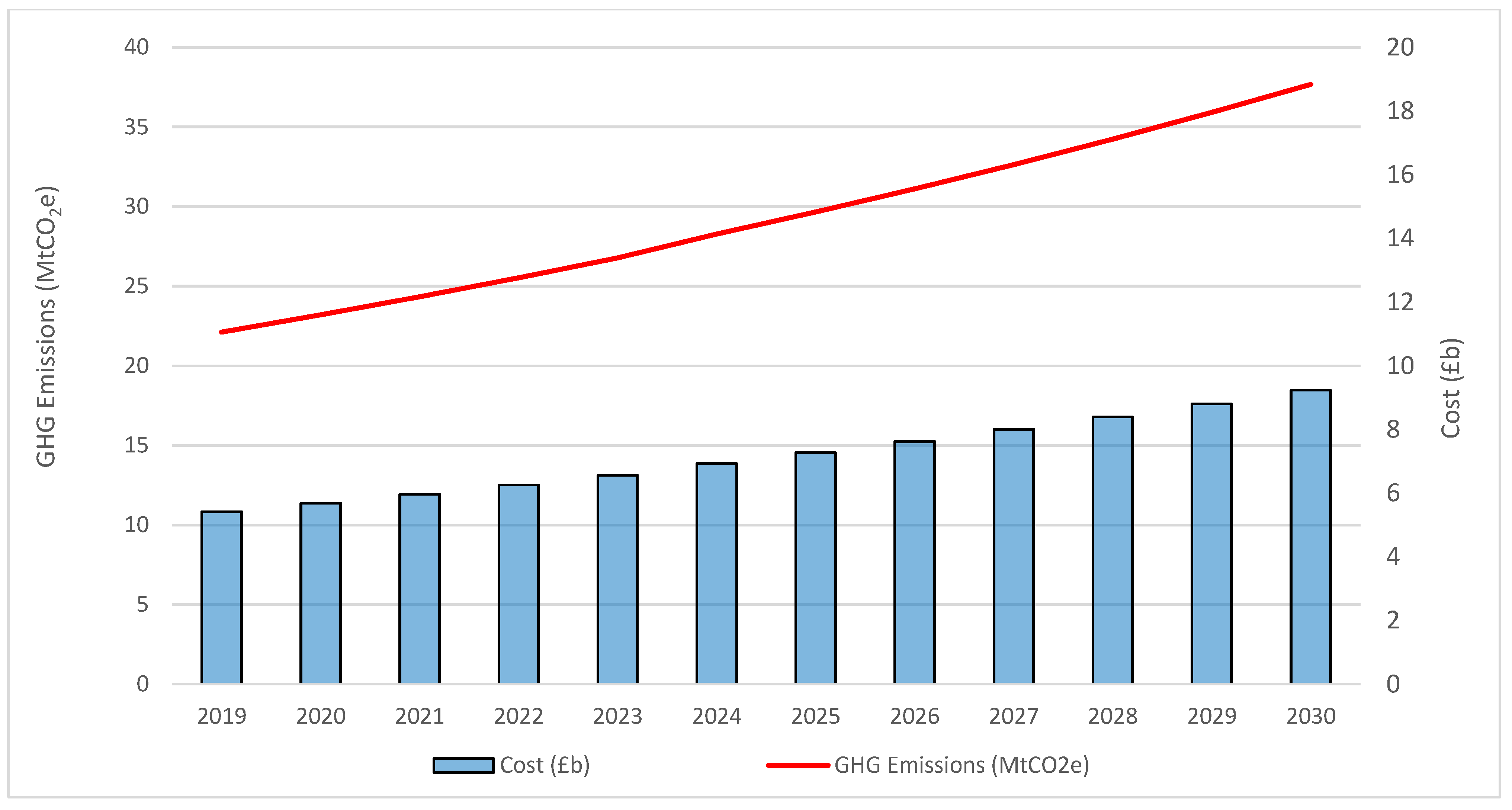
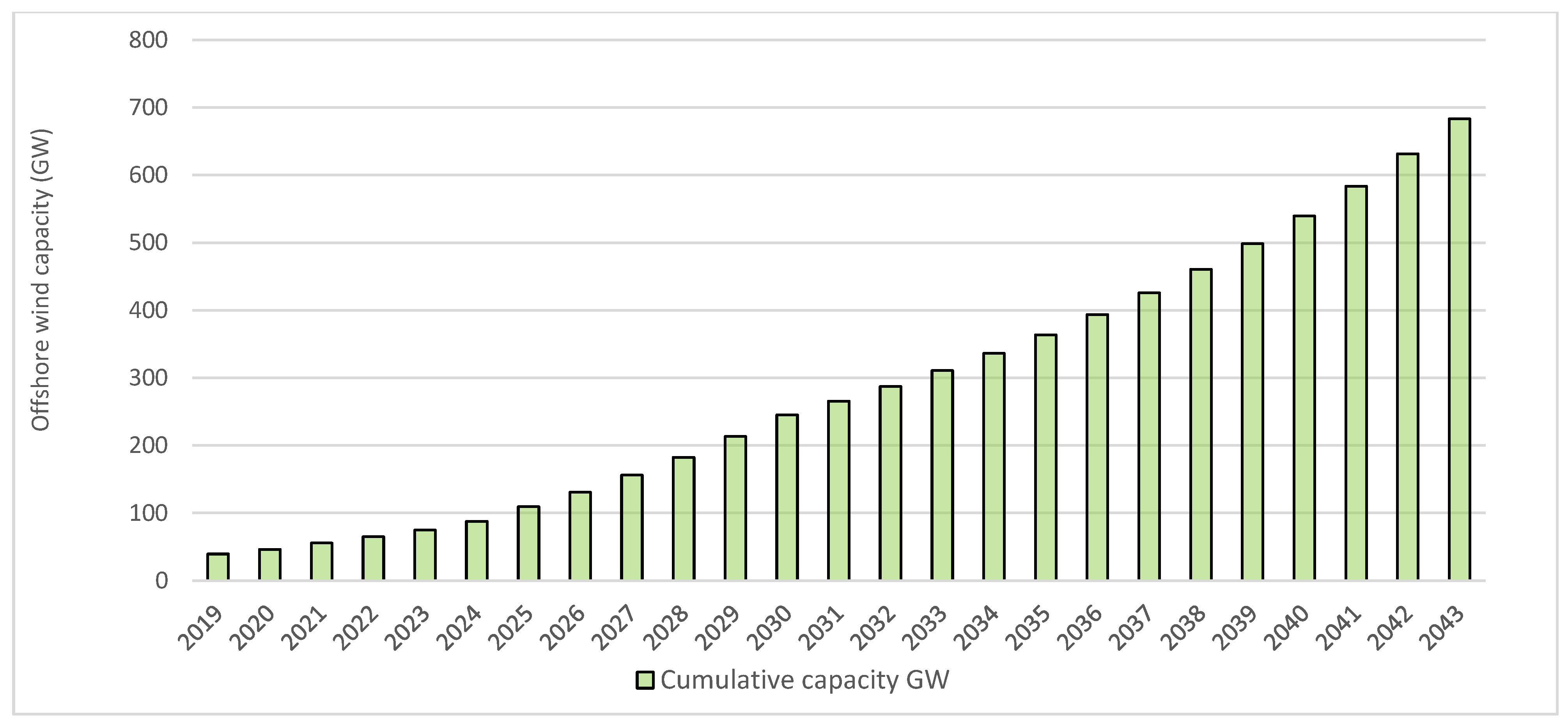
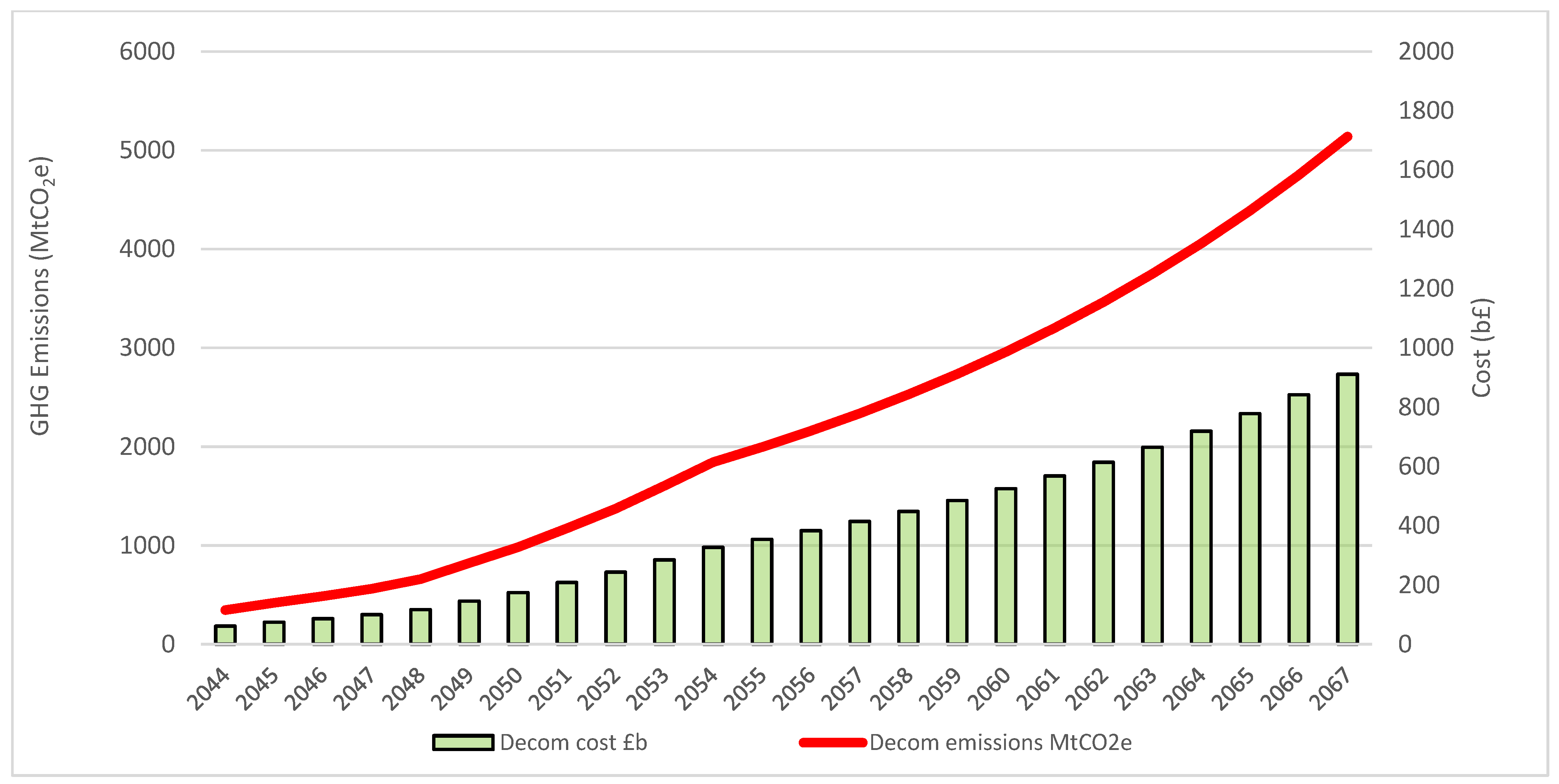
3.5. Global Decommissioning Future Trends
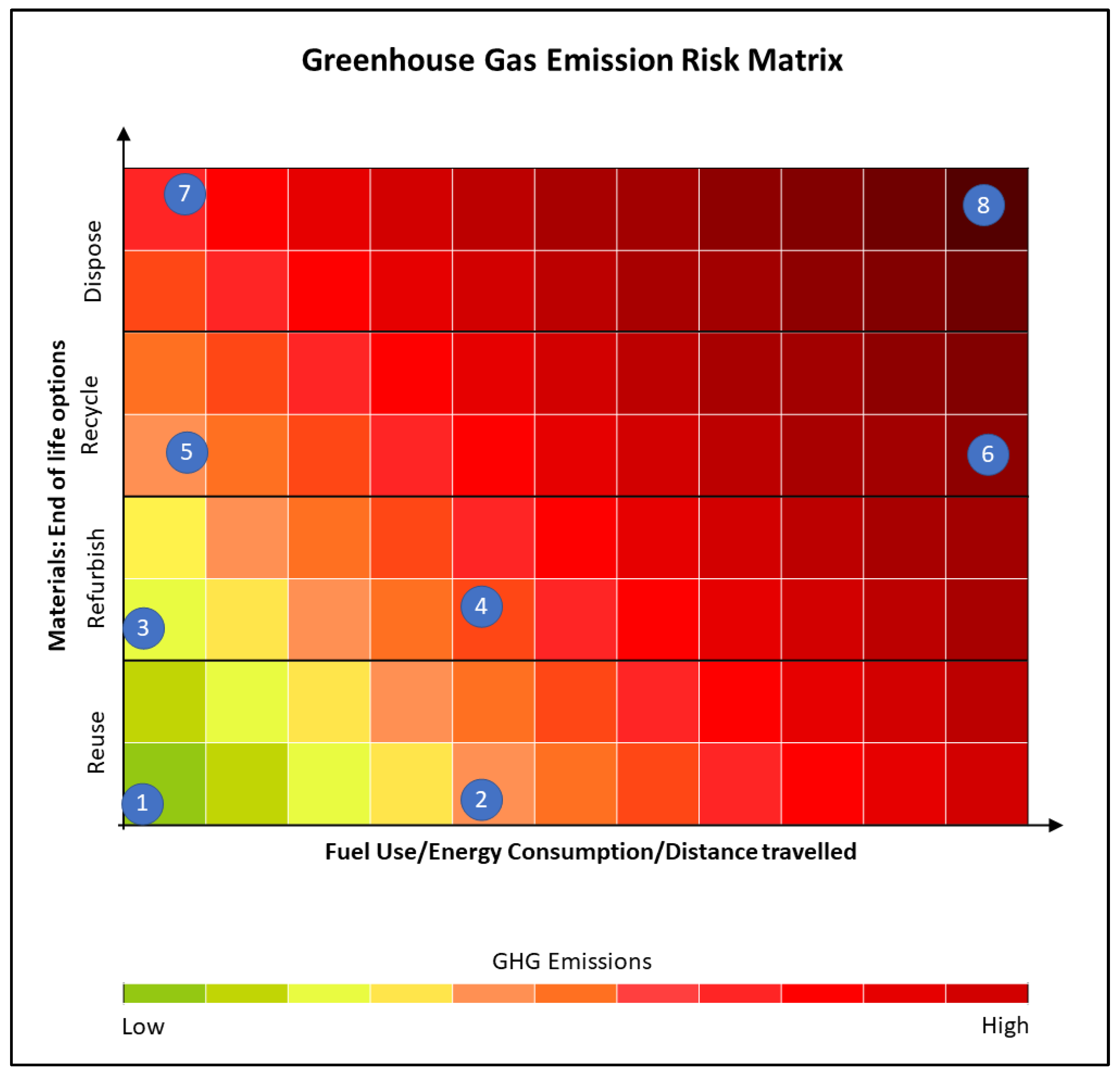
3.6. Emissions Risk Matrix
4. Discussion
5. Conclusions
- The work presented here shows that current OGI decommissioning GHG emissions calculation methods are underreporting GHG emissions by at least half.
- It illustrates that the impact of decommissioning offshore infrastructure on global heating is currently significant at 25 MtCO2e, 0.5% of annual global GHG emissions and that these emissions will increase 200-fold over the coming decades to at least 5 GtCO2e by 2067; 17 years after Net Zero emissions should have been achieved, which is not compatible with the Paris Agreement.
- The work demonstrates that to understand GHG emissions reduction targets, accurate baseline emissions are required, without which the scale of reduction targets is not understood, nor can effective decarbonization strategies be applied.
- New guidelines are urgently required to allow for accurate pre-decommissioning GHG emissions figures to be calculated and a ‘close-out report’ to be submitted after decommissioning has taken place so that realistic GHG emissions figures can be determined. This should be consistently applied to all industries with infrastructure in the marine environment, including both the OGI and the renewables industry and across all countries.
- New GHG emissions quantification methods should be developed to ensure all consequential GHG emissions from decommissioning are captured and reported accurately, the results of which should be easily accessible and understandable to the general public.
- The results presented here reveal the true scale of the challenge that decommissioning presents and that current decommissioning methods based on clear seabed policies are not compatible with the Paris Agreement.
Author Contributions
Funding
Data Availability Statement
Conflicts of Interest
References
- Gourvenec, S.; Sturt, F.; Reid, E.; Trigos, F. Global Assessment of Historical, Current and Forecast Ocean Energy Infrastructure: Implications for Marine Space Planning, Sustainable Design and End-of-Engineered-Life Management. Renew. Sustain. Energy Rev. 2022, 154, 111794. [Google Scholar] [CrossRef]
- OSPAR Commission. OSPAR Decision 98/3 on the Disposal of Disused Offshore Installations. 1998. Available online: https://www.ospar.org/work-areas/oic/installations (accessed on 10 February 2023).
- Institute of Petroleum (IOP). Guidelines for the Calculation of Estimates of Energy Use and Gaseous Emissions in the Decommissioning of Offshore Structures; Institute of Petroleum: London, UK, 2000. [Google Scholar]
- Davies, A.J.; Hastings, A. Quantifying Greenhouse Gas Emissions from Decommissioned Oil and Gas Steel Structures: Can Current Policy Meet NetZero Goals? Energy Policy 2022, 160, 112717. [Google Scholar] [CrossRef]
- DNV. Energy Transition Outlook; DNV: Greater Oslo, Norway, 2022. [Google Scholar]
- OEUK. Decommissioning Insight 2022; Offshore Energies UK (OEUK): London, UK, 2022. [Google Scholar]
- Oil&Gas. Global Oil & Gas Decommissioning Costs to Total $42 Billion through 2024. Available online: https://www.oilandgasmiddleeast.com/exploration-production/drilling-production/36687-global-oil-gas-decommissioning-costs-to-total-42-billion-through-2024 (accessed on 10 January 2023).
- Market Research Future. Global Offshore Wind Market Overview. Available online: https://www.marketresearchfuture.com/reports/offshore-wind-market-3284#:~:text=Offshore%20Wind%20Market%20Size%20was%20valued%20at%20USD,21.0%25%20during%20the%20forecast%20period%20%282022%20-%202030%29 (accessed on 10 February 2023).
- World Economic Forum. The Winds of Change: 5 Charts on the Future of Offshore Wind Energy. Available online: https://www.weforum.org/agenda/2020/08/offshore-wind-energy-growth-energy-transition/ (accessed on 10 February 2023).
- GWEC. Global Offshore Wind Report 2020; Global Wind Energy Council: Brussels, Belgium, 2020. [Google Scholar]
- Statista. Offshore Wind Energy Capacity Worldwide from 2009 to 2021. Available online: https://www.statista.com/statistics/476327/global-capacity-of-offshore-wind-energy/ (accessed on 14 April 2023).
- Creswell, J. Offshore Wind Starts Squaring up to Massive Future Decom Challenge. Energy Voice. Available online: https://www.energyvoice.com/renewables-energy-transition/wind/uk-wind/274744/offshore-wind-starts-squaring-up-to-massive-future-decom-challenge/ (accessed on 10 January 2023).
- IEA. Renewables 2020 Analysis and Forecast to 2025; International Energy Agency: Paris, France, 2020.
- Statista. Market Value of Offshore Decommissioning Worldwide in 2019 and 2024. Available online: https://www.statista.com/statistics/326070/global-offshore-decommissioning-market-size/ (accessed on 10 February 2023).
- International Energy Agency. Renewable Energy Market Update; International Energy Agency: Paris, France, 2022.
- TAQA. North Cormorant Topsides Environmental Appraisal. 2020. Available online: https://assets.publishing.service.gov.uk/government/uploads/system/uploads/attachment_data/file/936723/North_Cormorant_Topsides_Decommissioning_Programme_-_Final.pdf (accessed on 20 February 2023).
- TAQA. Tern Topsides Environmental Appraisal. 2020. Available online: https://assets.publishing.service.gov.uk/government/uploads/system/uploads/attachment_data/file/936665/Tern_Topsides_Decommissioning_Programme_-_Final.pdf (accessed on 20 February 2023).
- Equinor. PL301 Heimdal to Brae Alpha Condensate Pipeline EA. 2021. Available online: https://assets.publishing.service.gov.uk/government/uploads/system/uploads/attachment_data/file/982471/PL301_-_Decommissioning_Programme.pdf (accessed on 20 February 2023).
- Shell UK Ltd. Gaupe Environmental Appraisal. 2021. Available online: https://assets.publishing.service.gov.uk/government/uploads/system/uploads/attachment_data/file/985670/Gaupe_Decommissioning_Programme_-_Approval_Version.pdf (accessed on 20 February 2023).
- Repsol Sinopec. Buchan & Hannay EA. 2020. Available online: https://assets.publishing.service.gov.uk/government/uploads/system/uploads/attachment_data/file/971600/BUCHAN_AND_HANNAY_DECOMMISSIONING_PROGRAMME_05.PDF (accessed on 20 February 2023).
- Spirit Energy. Ensign EA; Spirit Energy: London, UK, 2021. [Google Scholar]
- INEOS. Windermere Environmental Statement. 2021. Available online: https://assets.publishing.service.gov.uk/government/uploads/system/uploads/attachment_data/file/975529/RD-WIN-ZPL001_Rev11_WIN_Decommissioning_Programme_18MAR2021_FINAL.pdf (accessed on 20 February 2023).
- Marathon Oil. East Brae and Braemar ES & Technical Appendix. 2020. Available online: https://assets.publishing.service.gov.uk/government/uploads/system/uploads/attachment_data/file/922820/East_Brae_Topsides_and_Braemar_DP.pdf (accessed on 20 February 2023).
- Marathon Oil. Brae Alpha ES & Technical Appendix; Marathon Oil: Houston, TX, USA, 2017. [Google Scholar]
- Shell UK Ltd. Brent ES & ES Appendix; Shell UK Ltd.: London, UK, 2017. [Google Scholar]
- Hess Ltd. Atlantic & Cromarty EIA; Hess Ltd.: Singapore, 2016. [Google Scholar]
- Ithaca Energy Ltd. Anglia EA. 2020. Available online: https://assets.publishing.service.gov.uk/government/uploads/system/uploads/attachment_data/file/892416/Anglia_Decommissioning_Programme.pdf (accessed on 20 February 2023).
- Whiteley, L.; Axon, S. Alma & Galia Decommissioning Environmental Appraisal; EnQuest: London, UK, 2020. [Google Scholar]
- Lundin Energy. Brynhild Field Decommissioning Project: Environmental Appraisal. 2020. Available online: https://assets.publishing.service.gov.uk/government/uploads/system/uploads/attachment_data/file/891522/Brynhild_Decommissioning_Programme.pdf (accessed on 20 February 2023).
- INEOS UK. Cavendish Decommissioning Environmental Appraisal. INEOS UK SNS Limited. 2019. Available online: https://assets.publishing.service.gov.uk/government/uploads/system/uploads/attachment_data/file/889054/RD-CAV-ZPL004_Rev07_CAV_Decommissioning_Programme_May2020_FINAL.pdf (accessed on 20 February 2023).
- Chrysaor. Caister Decommissioning Programmes: CDP1a; Chrysaor: London, UK, 2020. Available online: https://assets.publishing.service.gov.uk/government/uploads/system/uploads/attachment_data/file/877103/Caister_-_CDP1.pdf (accessed on 20 February 2023).
- TAQA. Cormorant Alpha Derrick Decommissioning Environmental Appraisal. 2020. Available online: https://assets.publishing.service.gov.uk/government/uploads/system/uploads/attachment_data/file/890016/Cormorant_Alpha_Derrick_Structure_Removal_and_MDR_Installation_Decommissioning_Programme_-_FINAL__03-06-20___004_.pdf (accessed on 20 February 2023).
- Spirit Energy. South Morecambe DP3-DP4 Decommissioning Environmental Appraisal; Spirit Energy: London, UK, 2018. [Google Scholar]
- TAQA. Eider Topsides Decommissioning Environmental Appraisal; TAQA: Abu Dhabi, United Arab Emirates, 2020. [Google Scholar]
- Chrysaor LOGGS Area Decommissioning; Chrysaor: London, UK, 2020; Available online: https://www.harbourenergy.com/media/fyzfdwpy/loggs-area-decommissioning-environmental-appraisal-to-loggs-ldp2-ldp5.pdf (accessed on 27 May 2023).
- ConocoPhillips. MacCulloch Field Decommissioning Project: Subsea Infrastructure and Associated Infield Pipelines. 2019. Available online: https://assets.publishing.service.gov.uk/government/uploads/system/uploads/attachment_data/file/844958/MacCulloch_Decommissioning_Programme.pdf (accessed on 20 February 2023).
- DNO. Schooner and Ketch Decommissioning Environmental Appraisal. 2019. Available online: https://assets.publishing.service.gov.uk/government/uploads/system/uploads/attachment_data/file/826988/Ketch_Decommissioning_Programme_BEIS_Final_July_2019.pdf (accessed on 20 February 2023).
- Neptune Energy. Juliet Decommissioning Environmental Appraisal. 2019. Available online: https://assets.publishing.service.gov.uk/government/uploads/system/uploads/attachment_data/file/822799/Juliet_Decommissioning_Programme.pdf (accessed on 20 February 2023).
- ConocoPhillips. Environmental Statement for the SNS Phase 1 Decommissioning Project: Viking VDP1 and LOGGS LDP1; ConocoPhillips: Houston, TX, USA, 2015. [Google Scholar]
- Fairfield Fagus. Merlin Subsea Decommissioning Environmental Statement. 2017. Available online: https://assets.publishing.service.gov.uk/government/uploads/system/uploads/attachment_data/file/668455/Merlin_Final_DP.pdf (accessed on 20 February 2023).
- Fairfield Fagus. Osprey Subsea Decommissioning Environmental Statement. 2017. Available online: https://assets.publishing.service.gov.uk/government/uploads/system/uploads/attachment_data/file/668411/Osprey_Final_DP.pdf (accessed on 20 February 2023).
- Fairfield. Dunlin Subsea Decommissioning Environmental Statement; Fairfield: Westhill, UK, 2017. [Google Scholar]
- Spirit Energy. Markham ST-1 Decommissioning Environmental Impact Assessment. 2018. Available online: https://assets.publishing.service.gov.uk/government/uploads/system/uploads/attachment_data/file/693560/Markham_ST-1.pdf (accessed on 20 February 2023).
- Repsol. Rev UKCS Decommissioning Project; Repsol: Singapore, 2017. [Google Scholar]
- Spirit Energy. A-Fields Decommissioning Saturn (Annabel) and Audrey Fields Environmental Impact Assessment; Spirit Energy: London, UK, 2017. [Google Scholar]
- Spirit Energy. A-Fields Decommissioning Ann and Alison Fields Environmental Impact Assessment. 2018. Available online: https://assets.publishing.service.gov.uk/government/uploads/system/uploads/attachment_data/file/704216/Ann_and_Alison_Approved_Decommissioning_Programmes.pdf (accessed on 20 February 2023).
- Centrica. Ann A4 Installation Decommissioning Environmental Impact Assessment; Centrica: Windsor, UK, 2016. [Google Scholar]
- Nexen Petroleum UK. Environmental Impact Assessment for the Decommissioning of the Ettrick and Blackbird Field Developments; ETRK0001-GE-O000-LC-RPT-0006; Nexen Petroleum U.K. Limited: Uxbridge, UK, 2016. [Google Scholar]
- Ithaca Energy Ltd. Athena Field Decommissioning Programmes. 2016. Available online: https://assets.publishing.service.gov.uk/government/uploads/system/uploads/attachment_data/file/558359/Athena_Decommissioning_Programmes.pdf (accessed on 20 February 2023).
- Maersk Oil. Janice, James and Affleck Decommissioning Programmes. 2016. Available online: https://assets.publishing.service.gov.uk/government/uploads/system/uploads/attachment_data/file/562398/Janice_James_and_Affleck_Decommissioning_Programmes_Final.pdf (accessed on 25 April 2023).
- Perenco UK Limited. Tyne Installation Decommissioning programme Environmental Impact Assessment. 2019. Available online: https://assets.publishing.service.gov.uk/government/uploads/system/uploads/attachment_data/file/773414/Tyne_Decommissioning_Programme_INSTALLATION__Final_Version_Issued.pdf (accessed on 20 February 2023).
- Perenco UK Limited. Guinevere Installation Decommissioning Project Environmental Impact Assessment. 2019. Available online: https://assets.publishing.service.gov.uk/government/uploads/system/uploads/attachment_data/file/773415/Guinevere_Installation_Decommissioning_Programme_-_Final_Version_Issue.pdf (accessed on 20 February 2023).
- Maersk Oil. Leadon Decommissioning Environmental Statement. 2015. Available online: https://assets.publishing.service.gov.uk/government/uploads/system/uploads/attachment_data/file/504535/Leadon_Decommissioning_Programmes_.pdf (accessed on 20 February 2023).
- Shell UK Ltd. Curlew Decommissioning Environmental Statement; Shell UK Ltd.: London, UK, 2018. [Google Scholar]
- Ithaca Energy Ltd. Jacky Decommissioning Environmental Impact Assessment; Ithaca Energy Ltd.: London, UK, 2015. [Google Scholar]
- Bains Decommissioning Environmental Appraisal. 2018. Available online: https://assets.publishing.service.gov.uk/government/uploads/system/uploads/attachment_data/file/772043/Bains_Decommissioning_Programmes.pdf (accessed on 20 February 2023).
- ConocoPhillips. ES for SNS Decommissioning Programme: Viking VDP2 and VDP3; ConocoPhillips: Houston, TX, USA, 2018. [Google Scholar]
- Endeavour. Environmental Statement for the Decommissioning of the Rubie/Renee Facilities. 2014. Available online: https://assets.publishing.service.gov.uk/government/uploads/system/uploads/attachment_data/file/286701/RR_Decommissioning_Programme.pdf (accessed on 20 February 2023).
- ConocoPhillips. Close Out Report for Viking VDP1 and LOGGS LDP1 Decommissioning; ConocoPhillips: Houston, TX, USA, 2018. [Google Scholar]


Disclaimer/Publisher’s Note: The statements, opinions and data contained in all publications are solely those of the individual author(s) and contributor(s) and not of MDPI and/or the editor(s). MDPI and/or the editor(s) disclaim responsibility for any injury to people or property resulting from any ideas, methods, instructions or products referred to in the content. |
© 2023 by the authors. Licensee MDPI, Basel, Switzerland. This article is an open access article distributed under the terms and conditions of the Creative Commons Attribution (CC BY) license (https://creativecommons.org/licenses/by/4.0/).
Share and Cite
Davies, A.J.; Hastings, A. Greenhouse Gas Emissions from Decommissioning Manmade Structures in the Marine Environment; Current Trends and Implications for the Future. J. Mar. Sci. Eng. 2023, 11, 1133. https://doi.org/10.3390/jmse11061133
Davies AJ, Hastings A. Greenhouse Gas Emissions from Decommissioning Manmade Structures in the Marine Environment; Current Trends and Implications for the Future. Journal of Marine Science and Engineering. 2023; 11(6):1133. https://doi.org/10.3390/jmse11061133
Chicago/Turabian StyleDavies, Abigail J., and Astley Hastings. 2023. "Greenhouse Gas Emissions from Decommissioning Manmade Structures in the Marine Environment; Current Trends and Implications for the Future" Journal of Marine Science and Engineering 11, no. 6: 1133. https://doi.org/10.3390/jmse11061133
APA StyleDavies, A. J., & Hastings, A. (2023). Greenhouse Gas Emissions from Decommissioning Manmade Structures in the Marine Environment; Current Trends and Implications for the Future. Journal of Marine Science and Engineering, 11(6), 1133. https://doi.org/10.3390/jmse11061133