Article

Temporal Prediction of Landslide-Generated Waves Using a Theoretical–Statistical Combined Method

1
School of Water Conservancy and Environment Engineering, Zhejiang University of Water Resources and Electric Power, Hangzhou 310018, China
2
College of Water Conservancy and Hydropower Engineering, Hohai University, Nanjing 210098, China
3
Environmental Hydraulics Laboratory, Ecole Polytechnique Fédérale de Lausanne, 1015 Lausanne, Switzerland
*
Authors to whom correspondence should be addressed.
J. Mar. Sci. Eng. 2023, 11(6), 1151; https://doi.org/10.3390/jmse11061151
Submission received: 22 April 2023 / Revised: 29 May 2023 / Accepted: 30 May 2023 / Published: 31 May 2023

Abstract

:
For the prediction of landslide-generated waves, previous studies have developed numerous empirical equations to express the maximums of wave characteristics as functions of slide parameters upon impact. In this study, we built the temporal relationship between the wave characteristics and slide features. We gave specific insights into impulse waves generated by snow avalanches and mimicked them using a buoyant material called Carbopol whose density is close to that of water. Using the particle image velocimetry (PIV) technique, the slide’s temporal velocity field and thickness, as well as the temporal free water surface fluctuation, were determined experimentally. Using a statistical method denoted as panel data analysis, we quantified the temporal wave amplitude from the time series data of the thickness and depth-averaged velocity of the sliding mass at the shoreline. Then, the slide’s temporal thickness and velocity at the shoreline were estimated from the parameters of the stationary slide at the initial position, based on the viscoplastic theory. Combining the panel data analysis and the viscoplastic theory, the temporal wave amplitudes were estimated from the initial slide parameters. In the end, we validated the proposed theoretical–statistical combined predictive method with the support of experimental data.

1. Introduction

When gravity-driven flows, such as avalanches, debris flows, and glacier calving, threaten surrounding bodies of water, such as oceans, lakes, and rivers, they can generate large impulse waves that have devastating effects. A recent event took place at Lake Askja, Iceland, in 2014, where a landslide of approximately 20 × 10 6 m 3 generated a large wave, reaching a height of 50 m, which inundated the shoreline by up to 80 m [1]. Another recent example was a rapid rock avalanche that occurred in 2017 in Greenland, where approximately 50 Mm 3 of landslide impacted the Karrat Fjord and created a wave that propagated 32 km to the village of Nuugaatsiaq [2]. In Switzerland, a cohesive avalanche had significant impact on a lake near Göschenen in 1999 [3]. The resulting snow–water mixture flowed out of the lake as a thick, viscous fluid, overtopped a 6-meter protection wall, and damaged the village structures.
The problem of impulse waves generated by subaerial landslides has attracted considerable attention in recent decades. Many of the physical insights into this phenomenon have come from laboratory-scale-down experiments [4,5,6,7,8,9,10], and to a lesser extent from theoretical models [11,12], numerical simulations [13,14,15,16,17], and field data surveys [18,19,20,21]. Laboratory experiments make it possible to quantify the maximum values of wave characteristics, such as the wave amplitude, wave height, and wave period from parameters of the incoming landslide using empirical equations. The most commonly used slide parameters in these empirical equations include the slide’s frontal velocity thickness across the shoreline and the slide mass, which were simplified from the momentum flux of the incoming landslide [22,23,24]. Using the slide’s frontal velocity and thickness as explanatory variables in empirical equations is effective, as many mass flows have their maximum velocity and thickness at the front, but it is not always the optimal solution. Natural landslides often have varying thicknesses and velocities from their front to tail, depending on the slide material properties, slope topography, etc. This shows the necessity of considering the time series data of slide parameters in wave prediction.
Furthermore, the transfer of momentum between the sliding mass and the body of water persists from the moment the slide’s frontal part touches the shoreline until the slide stops moving. The associated waves affect the surrounding area of water and structures throughout the whole impacting process rather than merely at the moment when the wave size reaches its maximum. Therefore, it is necessary to have a reliable prediction of the temporal wave characteristics instead of focusing solely on the maximum wave parameters. The time evolution of the wave characteristics has been widely explored in previous studies. The difficulty was to determine the time variation of the slide features experimentally. Several attempts have been conducted by recent research studies to determine the time series data of the slide parameters experimentally. Bullard et al. examined the temporal velocity of granular slides passing through shorelines [25]. Bougoin et al. determined the temporal evolution of gas-fluidized granular flows entering bodies of water [26]. However, no study has yet quantified the temporal relationship between the wave characteristics and slide features.
The objective of this study was to determine the temporal relationship between the wave characteristics and slide parameters. We provide specific insights into impulse waves generated by avalanches. The main characteristic of an avalanche, compared to other natural landslides, is its low density. We, thus, conducted experiments using a buoyant material called Carbopol, whose density is close to that of water. The choice of the material was detailed in our previous studies [27,28,29]. Using the particle image velocimetry (PIV) technique, the internal dynamics of the sliding mass as it passed through the shoreline were experimentally measured and, hence, the time series data of the slide’s velocity and thickness were determined.
Compared with previous empirical equations, which predicted the maximums of wave parameters, the challenge of this study was to model several variables at varying time points. In statistical and econometric research studies, three types of data were mostly used: cross-section data, time series data, and panel data [30,31]. Cross-section data are obtained by collecting observations related to many variables at given times. The experimental dataset, which was modeled by previous empirical equations, corresponds to this case. Only slide parameters upon impact and maximums of wave parameters were used in these empirical equations. Time series data consist of observations measured at many time points for one variable. For the temporal prediction in the present study, the dataset involves many variables at varying time points. In this case, panel data that combine cross-section data and time series data can be used. The panel data analysis has some benefits, such as increasing the number of observations and freedom degrees, and obtaining more efficient and consistent prediction results with more data information, which offer extended modeling possibilities compared to cross-sectional data or time-series data [32,33,34].
In this study, we first employed the panel data analysis to build the temporal relationship between the wave parameters and slide parameters upon impact. We then estimated the time series data of slide parameters upon impact from the features of the stationary slide material at the initial position based on the viscoplastic theory (i.e., lubrication model and kinematic wave model) [35,36]. Combining the panel data analysis with the viscoplastic theory, the temporal wave characteristics were predicted from the initial slide parameters. Compared with previous empirical equations, which predicted the maximum wave characteristics from slide parameters upon impact, the proposed statistical–theoretical combined model not only estimated the temporal parameters of the sliding mass upon impact but also predicted the temporal wave characteristics from these temporal slide parameters, which helps one to understand how the slide features affect wave generation.

2. Theoretical Basis

2.1. Physical Model

Figure 1 illustrates the physical model of a landslide moving down along a slope and entering a body of water. The whole process can be divided into three stages: (i) the slide is at rest in the container box and starts to move; (ii) it moves along the slope and then reaches the shoreline; (iii) it enters the body of water and generates a wave. We consider a slope with an inclination of θ entering a horizontal flume filled with water. The still water depth is denoted by h 0 . The landslide, with a volume of V I and density of ρ s , is released at a distance s from the shoreline. The sliding mass enters the body of water with a thickness of s 0 ( t ) and velocity of u 0 ( t ) . The characteristics of the wave generated by the sliding mass are represented by the wave amplitude a ( t ) and wave height h ( t ) .

2.2. Empirical Equations

Previous studies have developed a number of empirical equations to express the maximum values of wave characteristics, such as the wave amplitude, height, period, and length, as functions of parameters of the sliding mass upon impact [9,12,37,38,39,40,41,42]. The typical functional form of the empirical equations can be written as follows:
Y e = δ n = 1 X n β n
Y e ( e = 1 , 2 , ) are the scaled wave parameters (e.g., the scaled maximum wave amplitude, scaled maximum wave height, etc.), X n ( n = 1 , 2 , ) indicate the explanatory variables (i.e., scaled slide parameters), I represents the total number of explanatory variables, β n and δ denote the coefficients of the explanatory variables.
The most commonly used slide parameters in these empirical equations are the slide velocity u 0 , the slide thickness s 0 , and the effective slide mass m E , which were simplified from the momentum flux of the slide material passing through the shoreline. We define the mass of the immersed slide material as m, and the effective slide mass m E is the mass of the immersed slide material m at the moment when the wave height reaches its maximum [27]. s 0 and u 0 are the thickness and velocity of the sliding mass when its front touches the shoreline. These parameters are scaled as the slide Froude number Fr = u 0 / g h 0 , the scaled slide thickness S = s 0 / h 0 , the scaled effective mass M = m / ρ s B h 0 2 , with B as the slope width, ρ s as the slide density, and h 0 as the still water depth. Then, a commonly used simple empirical equation appears [24]:
Y e = δ Fr a M b S c
where δ , a, b, and c are the coefficients of explanatory variables and are estimated by regressing the equation using experimental data.

2.3. Slide Parameters Selected for the Temporal Prediction

As presented in Section 2.2, the slide’s thickness, velocity, and mass were routinely selected as representative slide parameters in empirical equations. According to the mass conservation, the change rate of the submerged slide mass d m d t can be expressed by the thickness and velocity of the sliding mass passing the shoreline:
d m d t = ρ s b s 0 ( t ) u 0 ( t )
where the slide density ρ s and the width of the flume b are constants. It means that the temporal mass of the submerged slide material m ( t ) depends on the thickness and velocity of the sliding mass passing through the shoreline (i.e., s 0 ( t ) and u 0 ( t ) ). Therefore, we eliminated the mass term for the temporal prediction.

3. Model Development

3.1. Panel Data Analysis

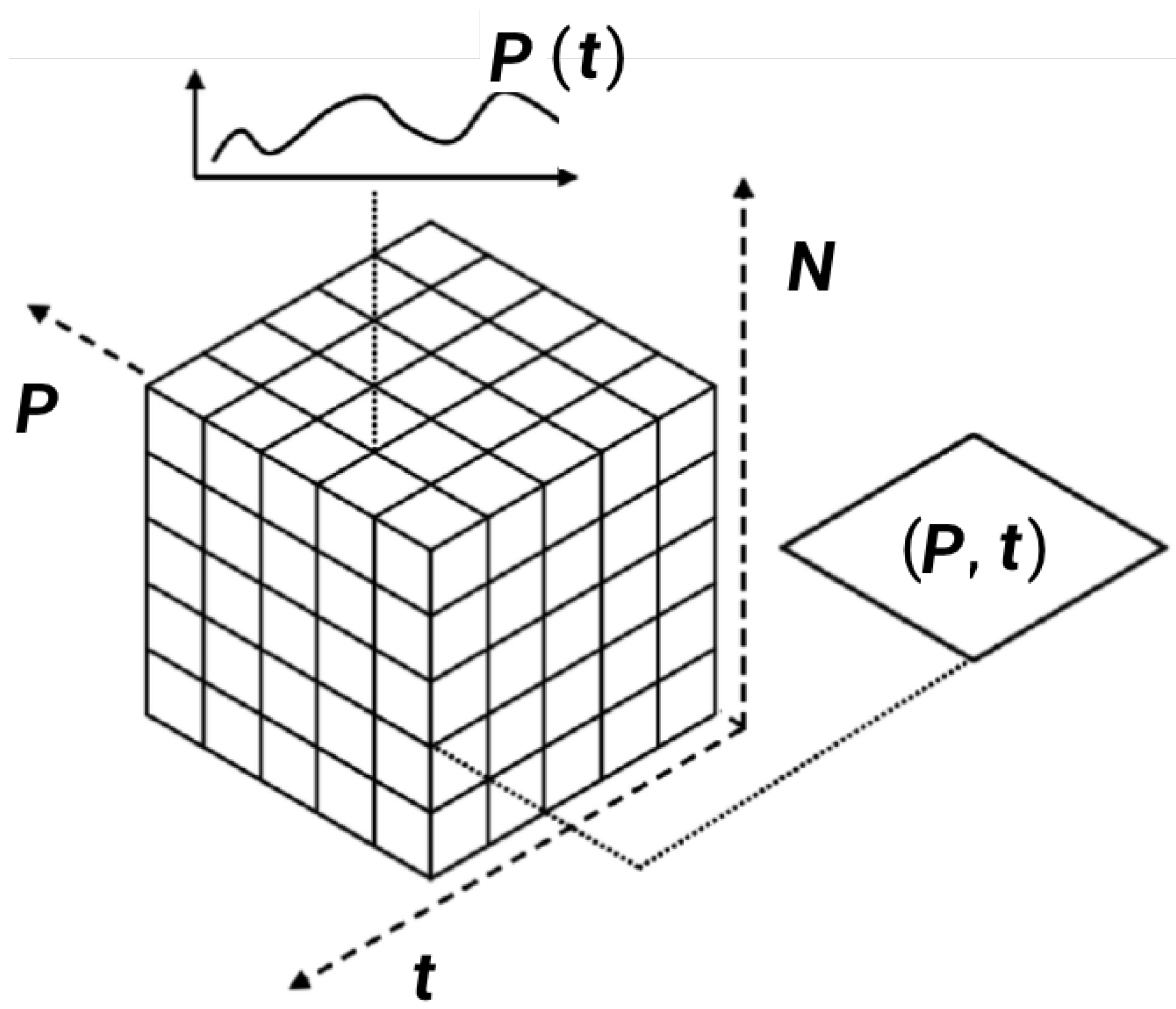
We built the temporal relationship between the wave parameters and slide parameters using panel data analysis, which enables multivariate regression analysis for a set of variables over a particular time span. As shown in Figure 2, our experimental data can be conceptualized as a three-dimensional dataset that contains a time series and a data panel N-P. N denotes the number of experiments and P denotes the slide parameters and wave parameters recorded in each experiment. The objective of this study was to quantify the time series data of wave parameters from slide parameters.
The random coefficient model proposed by Swamy (1970) was used to develop the temporal prediction [43]. The basic form of a panel data model is:
y i = X i β i + r i
There are T observations on each of the N individual units. The dimension of y i is ( T × 1 ) , the dimension of X i is ( T × Λ ) , the dimension of β i is ( Λ × 1 ) , and the dimension of r i is ( T × 1 ) . We observe the variables y i and X i for i = 1 , 2 , , N . The matrix X i ( i = 1 , 2 , , N ) has a of rank of Λ , containing observations on Λ non-stochastic regressors, denoted as x i t λ ( t = 1 , 2 , , T ; λ = 1 , 2 , , Λ ) . Both β i and r i are unobserved random vectors.
For the random coefficient model, let β i = β ¯ + γ i ( i = 1 , 2 , , N ) , where γ i is a Λ × 1 vector of the random elements. Swamy (1970) assumed that for i , j = 1 , 2 , , N :
E ( γ i ) = 0 , E ( γ i γ j ) = Δ , i = j , 0 , i j , E ( β i ) = β ¯ , E ( r i r j ) = σ i 2 I T i = j , 0 , i j .
In addition, β i and r j are independent, β i and β j for i j are independent. Equation (4) can be written as follows:
y = X β ¯ + D γ + r
where y = ( y 1 , y 2 , , y N ) , X = ( X 1 , X 2 , , X N ) , γ = ( γ 1 , γ 2 , , γ N ) , r = ( r 1 , r 2 , , r N ) , and D denotes a block-diagonal matrix. Under the assumptions of Equation (5), the N T × 1 disturbance vector D γ + r has the covariance matrix:
V = X 1 Δ X 1 + σ 1 2 I 0 X 2 Δ X 2 + σ 2 2 I 0 X N Δ X N + σ N 2 I
where the 0’s are T × T null matrices. The matrix V is symmetric with dimensions N T × N T , and ψ i = X i Δ X i + σ i 2 I . The optimal linear unbiased estimator of β can be obtained from the generalized least squares method:
β ^ G L S = i = 1 N X i ψ i 1 X i 1 i = 1 N X i ψ i 1 y i = i = 1 N W i β ^ i , W i = i = 1 N Δ + σ i 2 ( X i X i ) 1 1 1 Δ + σ i 2 ( X i X i ) 1 1 , β ^ i = X i X i 1 X i y i .
The variance–covariance matrix of the estimator β ^ G L S is as follows:
Var β ^ G L S = i = 1 N X i ψ i 1 X i 1 = i = 1 N Δ + σ i 2 ( X i X i ) 1 1 1 .
β ^ G L S is an effective estimation of β , which follows an asymptotic normal distribution.
Note that different wave types are often associated with different free water surface-moving tendencies; for instance, the wave amplitude of a bore wave increases and decreases much more quickly than that of a solitary wave during the moving landslide entering the body of water. These differences may result in uncertainties when modeling the three-dimensional panel data. In statistical and econometric studies, researchers commonly classify the dataset into several groups based on the properties of the data samples to avoid uncertainties. Here, we used a Gaussian mixture model to classify the experimental dataset based on the slide parameters upon impact before building the random coefficient model.
For multivariate continuous data, the parameterized component density is multivariate Gaussian density. For the one-dimensional dataset, the probability distribution of a random variable x follows a mixture of two Gaussian distributions:
P x | μ 1 , μ 2 , σ = k = 1 2 p k 1 2 π σ 2 exp x μ k 2 2 σ 2
where k = 1 and k = 2 represent two Gaussian distributions, the kth prior probability is p 1 = 1 / 2 , p 2 = 1 / 2 . Moreover, μ k and σ are the mean value and standard deviation of the two Gaussian distributions, respectively. We use θ = μ k , σ to represent these two parameters. The dataset x n n = 1 N contains N tests, which is an independent sample from the distribution.
Here, we consider that the μ k is unknown but σ is known; we can obtain μ k from the data series x n n = 1 N . We then derive the iterative algorithm of μ k to maximize the likelihood estimation:
P x n n = 1 N | μ k , σ = n P x n | μ k , σ .
Then, the natural logarithm of the likelihood L can be expressed as follows:
μ k L = n p k | n x n μ k σ 2 ,
where p k | n = P k n = k | x n , θ is the Gaussian density. Ignoring the items in μ k P k n = k | x n , θ , the second derivative versus μ k can be approximated as follows:
2 μ k 2 L = n p k | n 1 σ 2 .
The initial μ 1 , μ 2 are iterated to μ 1 , μ 2 using the approximate Newton–Raphson steps.
μ k = n p k | n x n n p k | n
The Gaussian mixture density of a multi-dimensional dataset (i.e., multiple Gaussian distribution) can be written as follows:
p k | n = π k 1 i = 1 I 2 π σ k exp i I μ k x n 2 / 2 σ k 2 k π k 1 i = 1 I 2 π σ k exp i I μ k x n 2 / 2 σ k 2 ,
where k is the serial number of the Gaussian distribution, n is the serial number of the data sequence, I is the total number of data dimensions, π k is the weighting, μ k is the mean value of the Gaussian distribution, σ k is the variance of the Gaussian distribution, and x n represents the data. The formulas of the standard derivation σ k and the weighting π k can be written as follows:
σ k = n p k | n x n μ k 2 n p k | n , π k = n p k | n k n p k | n

3.2. Theoretical Solutions of the Temporal Slide Thickness and Velocity

We provide insight into the cohesive landslide-generated waves and assume the incoming landslide as a viscoplastic fluid. The rheological behavior of the viscoplastic fluid is described by the Herschel–Bulkley equation [44,45]:
τ = τ c + μ γ ˙ n
where τ denotes the shear stress, τ c is the yield stress, γ ˙ is the shear rate, μ is the consistency, and n is a power law index that reflects shear thinning (or shear thickening for the materials n > 1). Independently of the constitutive equation, the shear stress distribution throughout the depth is as follows:
τ ( y ) = ρ s g ( s y ) sin θ
where s denotes the flow depth, ρ s is the density of the slide material, and g is the gravitational acceleration. The no-slip condition is assumed for the streamwise velocity component u at the bottom (i.e., u ( y = 0 ) = 0 ).
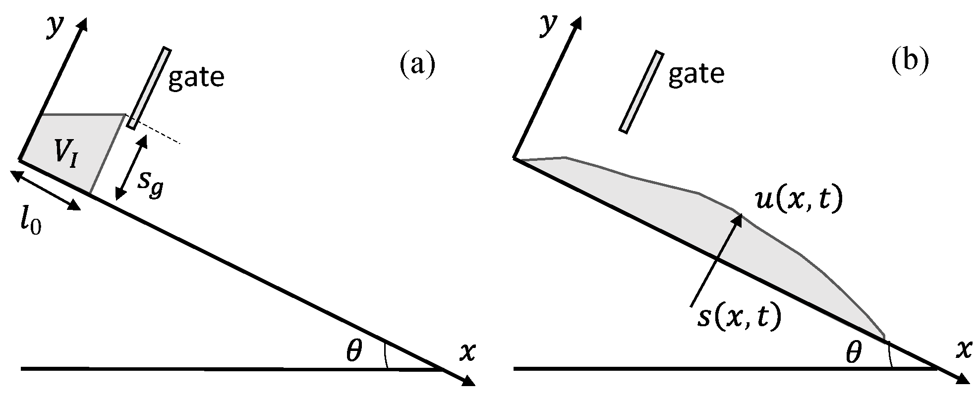
As shown in Figure 3, the slide moving along the slope can be considered as a dam break problem. The objective is to determine the thickness s ( x = l s , t ) (i.e., s 0 ( t ) ) and depth-averaged velocity u ¯ ( x = l s , t ) (i.e., u 0 ( t ) ), where l s represents the distance from the origin to the shoreline and t denotes the time. The initial flow depth s ( x ) is given by:
s ( x ) = s g + ( x l 0 ) tan θ
with s g = V I / l 0 + 1 2 l 0 tan θ , where s g is the initial flow depth at the lock gate, V I is the volume per width of the slide material in the container box, and l 0 denotes the length of the material in the reservoir.
The slide thickness s 0 ( t ) and depth-averaged velocity u 0 ( t ) crossing the shoreline are given by the lubrication model and kinematic wave model. Ancey et al. (2012) have detailed the models and validated them via experiments conducted with Carbopol [36]. For a slightly non-uniform viscoplastic flow, the depth-averaged velocity can be given by:
u ¯ = n K ( n + 1 ) ( 2 n + 1 ) tan θ s x 1 / n s ( n + 1 ) + n s c s Y 0 1 + 1 / n
with the parameter K = ρ s g cos θ / μ 1 / n , the updated yield surface position is given by Y 0 = s s c 1 cos θ s x 1 , and the critical depth is s c = τ c / ρ s g sin θ . Equation (20) requires an equation that specifies the gradient of the free surface x s ( x , t ) . We used the kinematic wave model to evaluate s ( x , t ) . The kinematic wave approximation assumes that the fluid is locally uniform. The integration of the constitutive Equation (17) provides the cross-stream velocity profile:
u ( y ) = n A n + 1 Y 0 1 + 1 / n ( Y 0 y ) 1 1 / n y Y 0 Y 0 1 + 1 / n y Y 0
with
Y 0 = s s c , A = ρ s g sin θ μ 1 / n , s c = τ c / ρ s g sin θ
where s c denotes the critical flow depth, i.e., no steady uniform flow is possible for s < s c . Y 0 denotes the position of the yield surface, where y < Y 0 corresponds to the sheared region and y > Y 0 corresponds to the unyielding region. Further integration leads to the depth-averaged velocity:
u ¯ = n A ( n + 1 ) ( 2 n + 1 ) s ( n + 1 ) + n s c s Y 0 1 + 1 / n
The bulk mass balance equation s t + s u ¯ x = 0 provides the governing equation for s:
s t + f ( s ) s x = 0
with f ( s ) = A s ( s s c ) 1 / n
This hyperbolic nonlinear advection equation can be solved easily using the characteristics method. Equation (24) can be put into a characteristic form d s d t ^ = 0 along the characteristic curve d x ^ d t ^ = f ( s ) . These initial characteristic curves are straight lines whose slopes are dictated by the initial depth:
x = f ( s ( x 0 ) ) t + x 0
with s 0 ( x 0 ) , the initial value of s at x 0 is given in Equation (19). As h = h 0 along the characteristic curve, using Equation (19) to eliminate x 0 , an implicit equation for s can be obtained:
x = A s ( s s c ) 1 / n t + ( s s g ) cot θ + l 0

4. Experiments

4.1. Facilities

Experiments were conducted in a narrow flume, which included two parts. The first part was a 1.5 m long and 0.12 m wide chute, which could be tilted at angles θ ranging from 30 to 50 . The bottom of the chute was lined with sandpaper, whereas the side walls were made of PVC. The second part was a 2.5 m long, 0.4 m deep, and 0.12 m wide transparent glass flume. The slide material was initially contained in a box located at the chute entrance and closed by a locked gate. In our experiments, the initial water depth was fixed to 0.2 m, the slope length s ranged from 0.85 m to 1.05 m, and the initial slide mass m I ranged from 2.0 to 6.0 kg. We conducted 92 experiments in total. Once the lock gate was released, the material accelerated energetically under gravity and reached velocities as high as 2.5 m/s. The thickness of the slide material passing through the shoreline ranged between 0.02 and 0.05 m.
As the slide material, we used a viscoplastic gel called Carbopol Ultrez 10. One benefit of Carbopol is that it is transparent and can be easily seeded with tracing particles without changing its rheological properties. This enables the measurement of its internal velocity using the particle image velocimetry (PIV) technique. The rheological behavior of Carbopol can be described by the Herschel–Bulkley equation (see Equation (17)). In this study, we used Carbopol with a concentration of 2.0%, with a yield stress of τ c = 58 Pa, a consistency of μ = 18.9 Pa·s n , and n = 0.330 . The density of Carbopol is close to 1000 kg/m 3 . For details on the material, refer to our earlier publications [27,28,29].
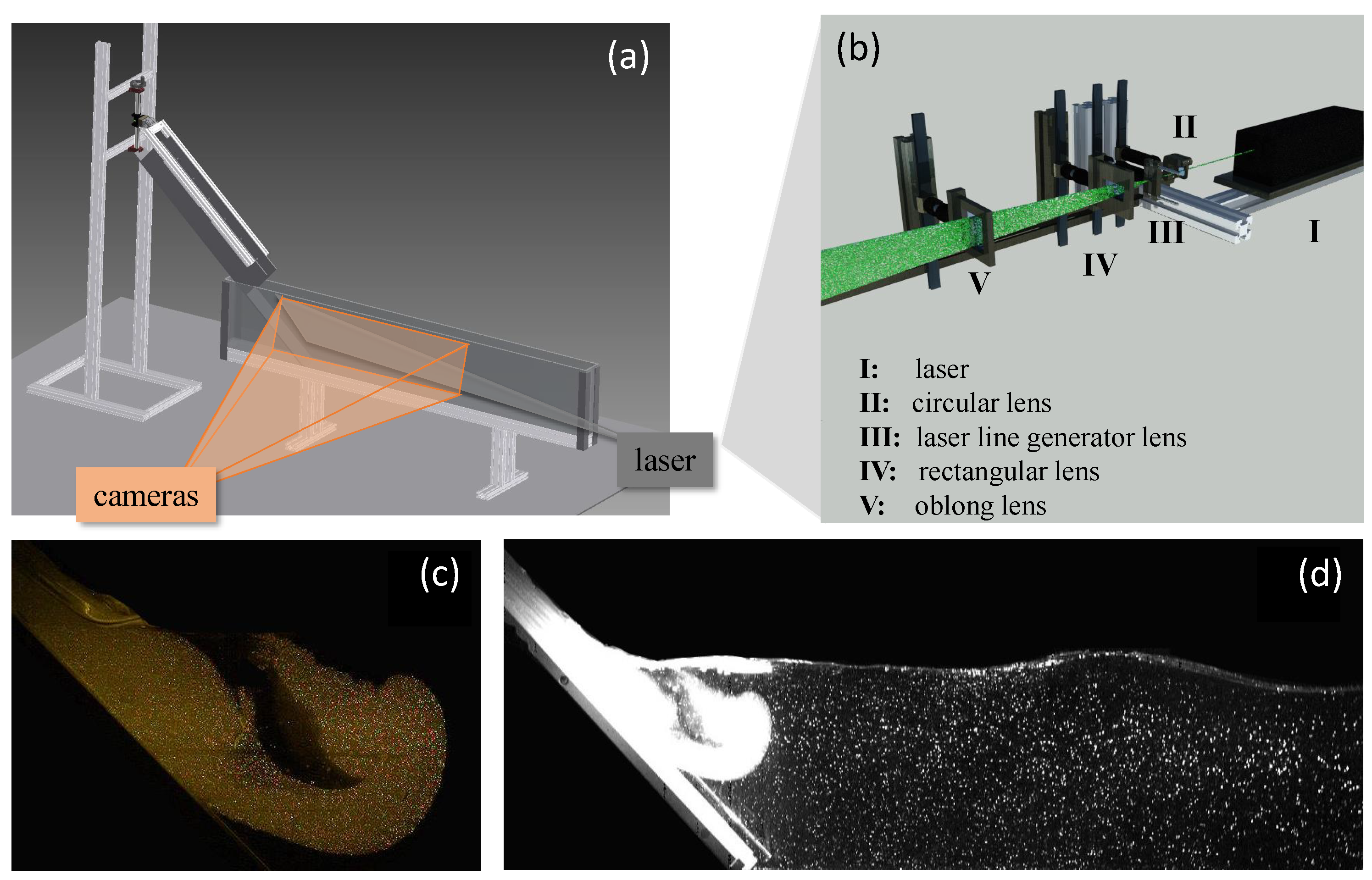
The flume was equipped with a PIV system, which consisted of a laser, four lenses, and two high-speed cameras. As illustrated in Figure 4a, the two cameras were placed in front of the shoreline with their optical axes perpendicular to the side wall, and the laser illumination system was installed on the opposite side of the slope. The laser generated a green laser beam with a wavelength of 527 nm, a maximum output of 150 W, and a pulse duration of 100 ns. As shown in Figure 4b, the laser beam first passed a circular lens (I) with a focal length of d =90 mm; it then passed through a laser line generator lens (II) with a divergence angle of 30 and it became a laser sheet; afterwards, the laser sheet passed through a rectangular lens (III) with a focal length of d = 200 mm in the vertical direction; finally, it passed by an oblong lens (IV) with a focal length of d = 1.5 m in the horizontal direction. We used a color camera with a frequency of 400 fps (frames per second) and a resolution of 600 × 800 pixels to record the motion of Carbopol (see Figure 4c) and a black-and-white camera with the same frequency and with a resolution of 1280 × 1024 pixels to record the motion of the body of water (see Figure 4d). Carbopol was seeded by fluorescent seeding particles with a diameter of 20 μ m; the particles were produced by mixtures of polyamide seeding particles and Rhodamine B dye. See [46] for details about the fluorescent seeding particles. Water was seeded by polyamide-seeding particles with a diameter of 50 μ m. The particle-seeded flow was illuminated in a target area with a light sheet, and the velocity vectors were derived from the sub-sections of the target area by measuring the displacement of seeding particles between two image frames.

4.2. Image Processing

The objective of the image processing is to obtain (1) the position of the free water surface when the leading wave reaches its maximum height, (2) the velocity and thickness of the sliding mass passing through the shoreline. To that end, we first located the interfaces among water, air, and the slide of each image. We then deduced the time variations of the wave characteristics by including the wave height and amplitude from the position of the free water surface, and determined the slide thickness from the slide-air interface.
The velocity field of the sliding mass was determined using a toolbox in Matlab named MatPIV. We used 32 × 32-pixel interrogation windows with 50% overlap between adjacent windows. To remove the spurious velocity vectors, a range validation filter was used, and all of the velocity vectors larger than 3 m/s were discarded. Using a moving average validation filter, the velocity vectors that deviate 15% from the average value of the surrounding 3 × 3 vectors fields were substituted by interpolation. The velocity vectors were converted into the velocities by calibrating the physical size of a pixel in an image. The depth-averaged velocity of the sliding mass passing through the shoreline was estimated by the average of the velocity vectors at the shoreline.

5. Results

5.1. Empirical Equations for Predicting the Maximums of Wave Characteristics

We selected the maximum wave amplitude a m and maximum wave height h m as representative wave parameters, and fitted the scaled maximum wave amplitude A m = a m / h 0 and the scaled maximum wave height H m = h m / h 0 with the slide Froude number Fr, scaled effective mass M, and scaled slide thickness S. In our experiments, 0.05 < Fr < 2.78, 0.03 < M < 0.33, and 0.12 < S < 0.25. The regression results of Equation (2) are as follows:
A m = 1.538 Fr 1.012 M 0.319 S 0.750
H m = 1.102 Fr 1.748 M 0.123 S 0.617
where the coefficient of determination is R 2 = 0.9214 for A m and 0.9062 for H m . Usually, a predictive model can be validated if R 2 > 0.8. As R 2 > 0.9 for both A m and H m , we believe that the prediction accuracies of the empirical equations were fairly good. The accuracy of the empirical equation of A m was higher than that of H m , which was commonly observed in most previous studies. Figure 5a,b compares A m and H m measured from experiments with those estimated by empirical Equations (28) and (29).

5.2. Time Series Data of the Slide Parameters Upon Impact

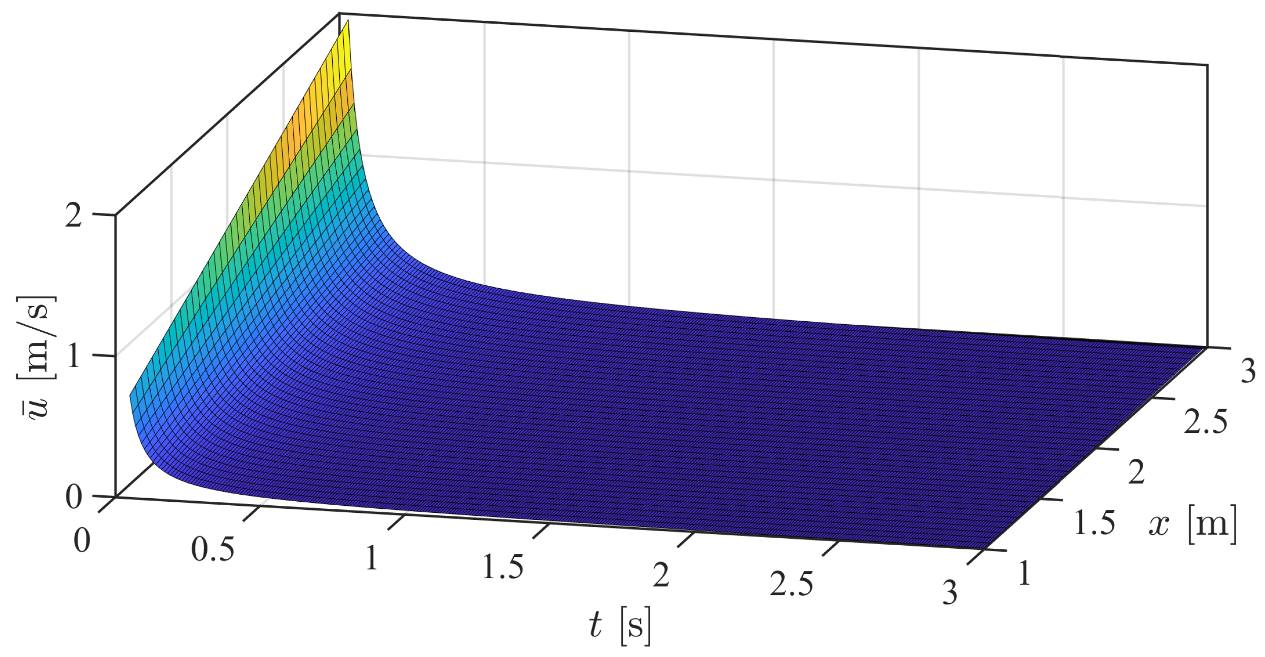
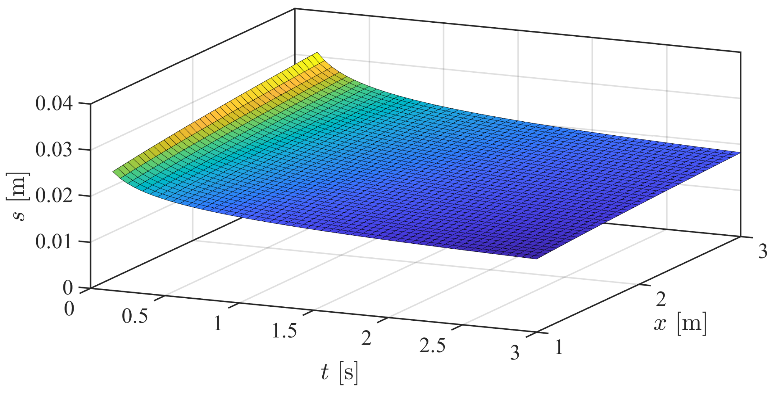
Using the theoretical expressions presented in Section 3.2, we calculate the numerical solutions of the time series data of the thickness and depth-averaged velocity of the sliding mass when it moves along the chute. Figure 6 and Figure 7 display the numerical solutions of s ( x , t ) and u ¯ ( x , t ) for the following specific case: θ = π / 6 , s g = 0.4 m, l 0 =0.3 m, l s = 0.85 m, n = 0.33 , τ c = 58 Pa, μ = 18.9 Pa·s n , g = 9.8 m/s 2 . The starting time counted for Equation (27) is given by x f ( t ) = l s .
Figure 8a,b display the time variation of s 0 ( t ) and u ¯ 0 ( t ) for the same selected cases as Figure 6 and Figure 7. Both s 0 ( t ) and u ¯ 0 ( t ) are determined experimentally and theoretically. The theoretical data are estimated with the lubrication model and kinematic wave model, and the experimental data are obtained from the PIV measurements (see Section 4). It can be seen from the figures that the theoretical data fit quite well with the experimental data. This confirms that the lubrication model and kinematic wave model can well represent the rheology of viscoplastic fluid.

5.3. Prediction of the Temporal Wave Characteristics

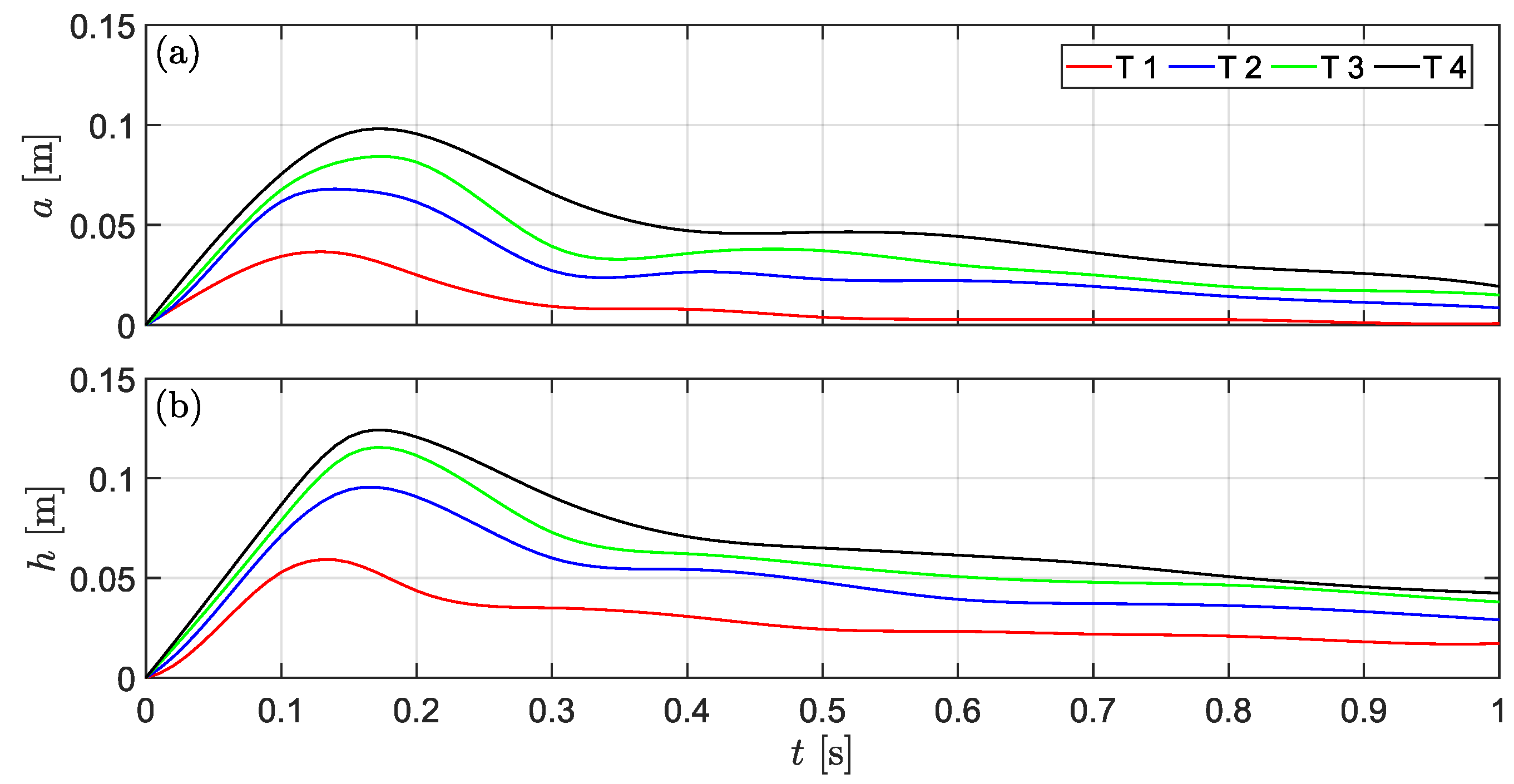
With the known s 0 ( t ) and u ¯ 0 ( t ) , we then quantify the temporal wave characteristics based on the panel data analysis. We first classify the experimental dataset into several groups using the Gaussian mixture model, and then use the random coefficient panel data model to model the time series relation between slide parameters and wave parameters. We selected four representative experiments as examples, and display the general tendencies of their surface evolution. Table 1 shows the initial parameters of the four selected experiments.
As shown in Figure 9, the varying tendencies of the four selected experiments are significantly different. The amplitude a ( t ) of T1 decreases after t = 1.5 s without any rally. For the evolution curve of a ( t ) of tests T2, T3, and T4, fluctuations can be observed during the decreasing period. For example, the a ( t ) of T2 starts to decrease at 0.15 s; it has a turning point of approximately 0.30 s. The discrepancies among experiments with different wave sizes increase the uncertainty of the temporal prediction. This uncertainty shows the necessity of clustering the dataset on the basis of the wave features and slide properties before conducting the temporal prediction.
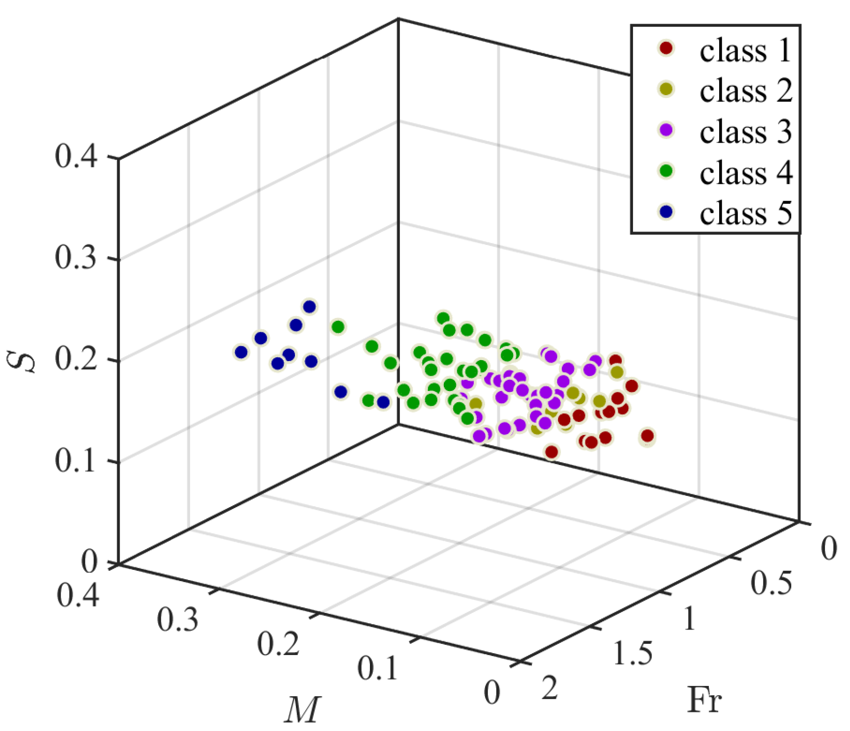
As shown in Section 5.1, the scaled maximum wave amplitude A m and scaled maximum wave height H m can be well estimated by the slide Froude number Fr, scaled slide thickness S, and scaled effective slide mass M using empirical equations, with the coefficient of determination R 2 larger than 0.9. We selected these three dimensionless groups as the criteria to evaluate the properties of experiments, and classified the experimental dataset using the Gaussian mixture model based on these three indicators. Figure 10 shows the classification results. Using the Gaussian mixture model, the 92 experiments conducted in the present study were classified into 5 classes: 14 experiments in class 1, 9 experiments in class 2, 30 experiments in class 3, 30 experiments in class 4, and 9 experiments in class 5.
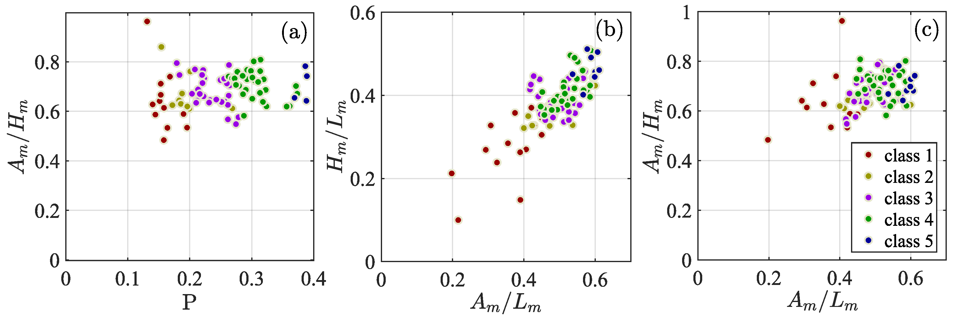
To verify whether the classification results well reflect the wave characteristics, we display the two-dimensional distribution of each class for the whole dataset. Figure 11a shows the impulse product parameter P versus the ratio of the scaled maximum wave amplitude to the scaled maximum wave height A m / H m . The impulse product parameter P was defined as P = Fr S 1 / 2 M 1 / 4 cos ( 6 / 7 θ ) 1 / 2 [47], and it was considered as a universal dimensionless group to quantify the wave characteristics. Therefore, P can generally reflect the size of the leading wave. In addition to A m / H m , Figure 11b,c display the ratio of A m and H m to the scaled wavelength L m ; that is, A m / L m and H m / L m , respectively. L m = / h 0 , where represents the wavelength. A m / H m , A m / L m , and H m / L m reflect the non-linearity of the wave. It can be seen that the classification results based on S, M, and Fr reflect the sizes and non-linearity of the waves.
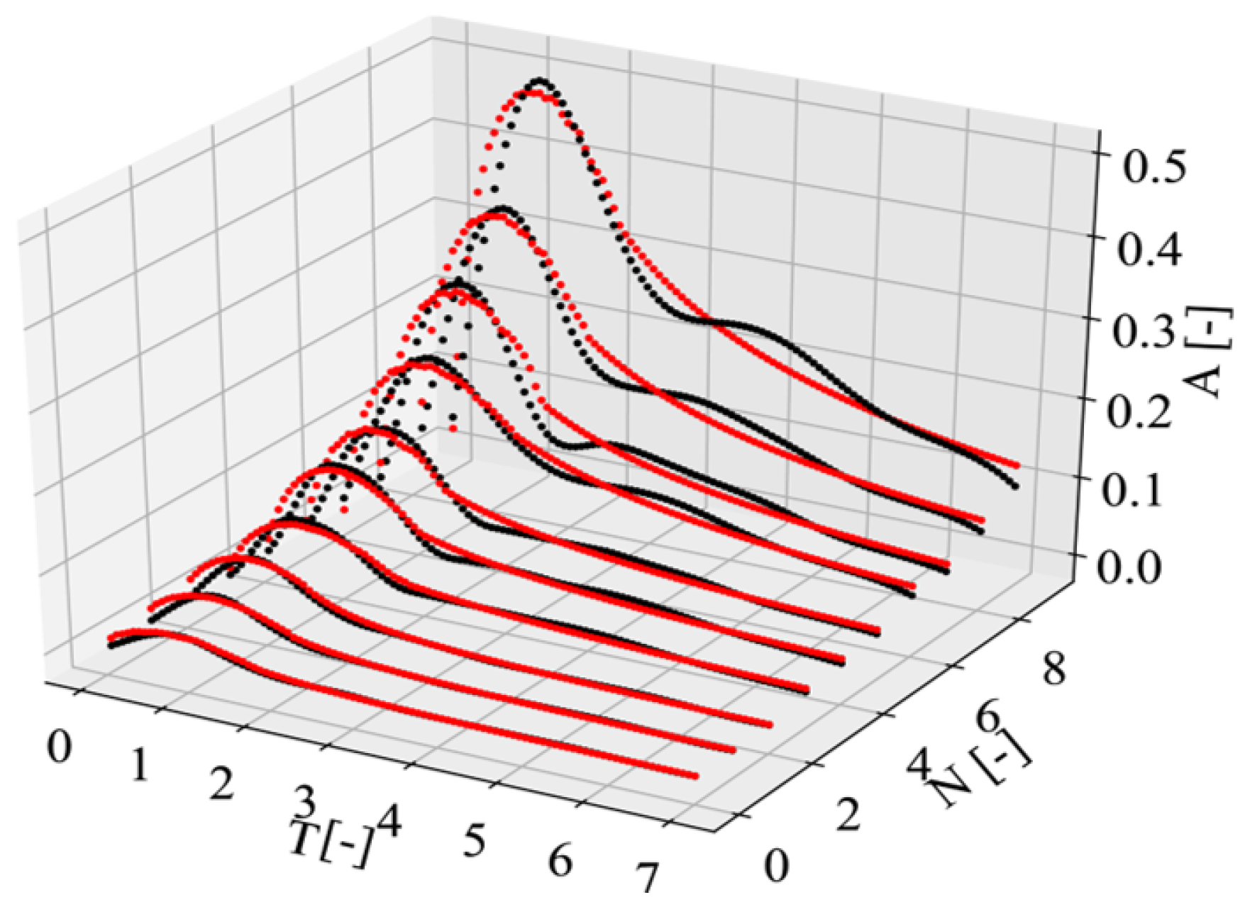
As the dataset has been classified, we now build the time series relation between the wave characteristics and slide parameters using the random coefficient model. See Section 3.1 for the mathematical details of the random coefficient model. We selected the wave amplitude a ( t ) to represent the temporal wave characteristics. The objective is to estimate A ( T ) from S ( T ) and Fr ( T ) , where A ( t ) = a ( t ) / h 0 is the scaled wave amplitude, S ( t ) = s 0 ( t ) / h 0 is the scaled slide thickness, Fr ( t ) = u 0 ( t ) / g h 0 is the Froude number, and T = t g / h 0 is the scaled time. Moreover, 82 of the 92 experiments were selected randomly to train the model, and the other 10 experiments were used to validate the model. Figure 12 shows A ( T ) of the 10 validation tests.
Further, as shown in Section 3.2 and Section 5.2, s 0 ( t ) and u 0 ( t ) can be estimated from the initial settings of the experiments using the kinematic wave model and lubrication model. We quantified the scaled temporal wave amplitude A ( T ) using the theoretical approximations of S ( T ) and Fr. Table 2 shows the prediction accuracy of A ( T ) of the 10 validation tests, with S ( T ) and Fr ( T ) given by experimental data and theoretical approximations, respectively. The prediction accuracy was evaluated by the coefficient of determination ( R 2 ) and mean square error (MSE) of the time series data sequence:
R 2 = 1 i = 1 ϵ y p , i y o , i 2 y p , i y ¯ o 2
MSE = i = 1 ϵ y p , i y o , i 2 ϵ
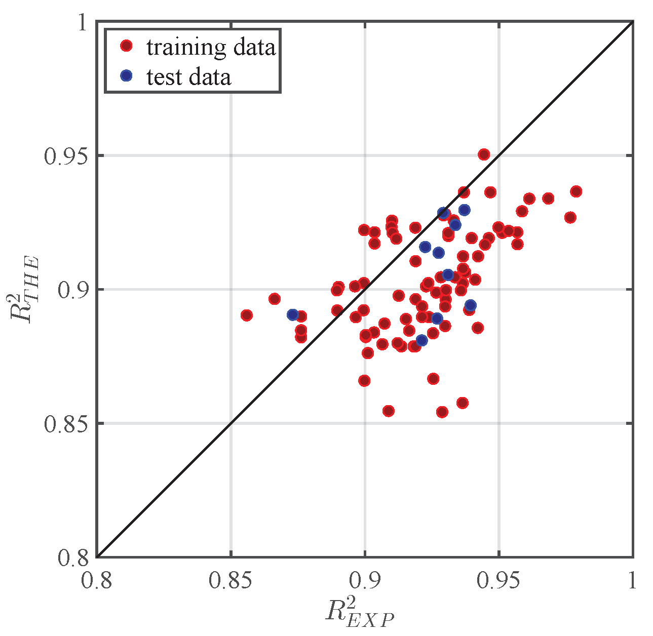
where ϵ is the sequence number of the experimental data, y p , i and y o , i are predicted and measured data, respectively, and y ¯ o is the average of the observed data. R E X P 2 and MSE E X P estimate the accuracies of the predictions with Fr and S given by the experimental data. R T H E 2 and MSE T H E estimate the accuracies of the predictions with Fr and S given by theoretical approximations. Since the R 2 values of most validation tests for A ( T ) were larger than 0.8, we believe that the proposed models perform well for quantifying the time series relations between the slide features and the wave characteristics.
Figure 13 shows the R T H E 2 and R E X P 2 values for the whole dataset. Using the experimental S ( T ) and Fr ( T ) to predict the temporal wave characteristics leads to better prediction accuracy than using theoretical approximations. The average R E X P 2 and R T H E 2 values of A ( T ) for the whole dataset were 0.9283 and 0.9045, respectively.

6. Conclusions

Previous studies have developed empirical equations to quantify the maximums of wave parameters, such as the maximum wave amplitude and maximum wave height from the slide parameters upon impact. No previous studies have quantified the temporal relationship between these parameters. The objective of this study was to establish the temporal relationship between the wave characteristics and slide features. In this study, we provided specific insight into impulse waves generated by snow avalanches. Considering the low density of snow avalanches, we selected a buoyant material called Carbopol as the slide material and conducted physical model experiments.
We selected the slide’s thickness and velocity at the shoreline as representative slide parameters. The time series data of these two slide parameters, as well as the wave fluctuations, were measured experimentally using the PIV technique. We quantified how the temporal wave amplitude depends on the time series data of the slide’s thickness and depth-averaged velocity as they pass through the shoreline, based on panel data analysis. The slide’s thickness and depth-averaged velocity were theoretically expressed using the lubrication model and kinematic wave model, derived from the initial parameters of the slide’s material in the container box. By combining the panel data analysis with the viscoplastic theory, we then quantified the time variation of the wave amplitude from the initial slide parameters. The proposed statistical–theoretical combined model demonstrated good agreement with the experimental data.

Author Contributions

Conceptualization, Z.M. and Y.H.; methodology, Y.H; validation, Z.M.; formal analysis, Z.M. and J.Z.; data curation, Z.M.; writing—original draft preparation, Z.M., J.Z. and Y.H.; writing—review and editing, Z.M. and J.Z.; supervision, C.A.; project administration, C.A.; funding acquisition, Z.M. and C.A. All authors have read and agreed to the published version of the manuscript.

Funding

This research was funded by the Chinese Postdoctoral Science Foundation (grant no. 2021M693679) and the Swiss National Science Foundation (grant no. 200021_146271/1).

Institutional Review Board Statement

Not applicable.

Informed Consent Statement

Not applicable.

Data Availability Statement

Data available upon request from the authors.

Conflicts of Interest

The authors declare no conflict of interest. The funders had no role in the design of the study; in the collection, analyses, or interpretation of data; in the writing of the manuscript; or in the decision to publish the results.

References

  1. Gylfadóttir, S.S.; Kim, J.; Helgason, J.K.; Brynjólfsson, S.; Höskuldsson, Á.; Jóhannesson, T.; Harbitz, C.B.; Løvholt, F. The 2014 Lake Askja rockslide-induced tsunami: Optimization of numerical tsunami model using observed data. J. Geophys. Res. Ocean. 2017, 122, 4110–4122. [Google Scholar] [CrossRef]
  2. Gauthier, D.; Anderson, S.A.; Fritz, H.M.; Giachetti, T. Karrat Fjord (Greenland) tsunamigenic landslide of 17 June 2017: Initial 3D observations. Landslides 2018, 15, 327–332. [Google Scholar] [CrossRef]
  3. Ammann, W. Der Lawinenwinter 1999: Ereignisanalyse; Eidgenössisches Institut für Schnee-und Lawinenforschung: Zurich, Switzerland, 2000. [Google Scholar]
  4. Huber, A.; Hager, W. Forecasting impulse waves in reservoirs. In Proceedings of the Transactions of The International Congress on Large Dams, Florence, Italy, 26–30 May 1997; Volume 1, pp. 993–1006. [Google Scholar]
  5. Fritz, H.M. Initial Phase of Landslide Generated Impulse Waves. Ph.D. Thesis, ETH Zurich, Zurich, Switzerland, 2002. [Google Scholar]
  6. Panizzo, A.; De Girolamo, P.; Petaccia, A. Forecasting impulse waves generated by subaerial landslides. J. Geophys. Res. Ocean 2005, 110. [Google Scholar] [CrossRef]
  7. Zweifel, A. Impulswellen: Effekte der Rutschdichte und der Wassertiefe. Ph.D. Thesis, ETH Zurich, Zurich, Switzerland, 2004. [Google Scholar]
  8. Heller, V.; Bruggemann, M.; Spinneken, J.; Rogers, B.D. Composite modelling of subaerial landslide–tsunamis in different water body geometries and novel insight into slide and wave kinematics. Coast. Eng. 2016, 109, 20–41. [Google Scholar] [CrossRef]
  9. McFall, B.C.; Mohammed, F.; Fritz, H.M.; Liu, Y. Laboratory experiments on three-dimensional deformable granular landslides on planar and conical slopes. Landslides 2018, 15, 1713–1730. [Google Scholar] [CrossRef]
  10. Evers, F.; Heller, V.; Fuchs, H.; Hager, W.H.; Boes, R. Landslide-Generated Impulse Waves in Reservoirs: Basics and Computation; VAW-Mitteilungen: Zurich, Switzerland, 2019; Volume 254. [Google Scholar]
  11. Di Risio, M.; Sammarco, P. Analytical modeling of landslide-generated waves. J. Waterw. Port Coast. Ocean Eng. 2008, 134, 53–60. [Google Scholar] [CrossRef]
  12. Zitti, G.; Ancey, C.; Postacchini, M.; Brocchini, M. Impulse waves generated by snow avalanches: Momentum and energy transfer to a water body. J. Geophys. Res. Earth Surf. 2016, 121, 2399–2423. [Google Scholar] [CrossRef]
  13. Watts, P. Water Waves Generated by Underwater Landslides. Ph.D. Thesis, California Institute of Technology, Los Angeles, CA, USA, 1997. [Google Scholar]
  14. Abadie, S.; Morichon, D.; Grilli, S.; Glockner, S. Numerical simulation of waves generated by landslides using a multiple-fluid Navier–Stokes model. Coast. Eng. 2010, 57, 779–794. [Google Scholar] [CrossRef]
  15. Yavari-Ramshe, S.; Ataie-Ashtiani, B. Numerical modeling of subaerial and submarine landslide-generated tsunami waves-recent advances and future challenges. Landslides 2016, 13, 1325–1368. [Google Scholar] [CrossRef]
  16. Yavari-Ramshe, S.; Ataie-Ashtiani, B. A rigorous finite volume model to simulate subaerial and submarine landslide-generated waves. Landslides 2017, 14, 203–221. [Google Scholar] [CrossRef]
  17. Ruffini, G.; Heller, V.; Briganti, R. Numerical modelling of landslide-tsunami propagation in a wide range of idealised water body geometries. Coast. Eng. 2019, 153, 103518. [Google Scholar] [CrossRef]
  18. Fritz, H.M.; Hillaire, J.V.; Molière, E.; Wei, Y.; Mohammed, F. Twin tsunamis triggered by the 12 January 2010 Haiti earthquake. Pure Appl. Geophys. 2013, 170, 1463–1474. [Google Scholar] [CrossRef]
  19. Grilli, S.T.; Grilli, A.R.; David, E.; Coulet, C. Tsunami hazard assessment along the north shore of Hispaniola from far-and near-field Atlantic sources. Nat. Hazards 2016, 82, 777–810. [Google Scholar] [CrossRef]
  20. Engel, M.; Oetjen, J.; May, S.M.; Brückner, H. Tsunami deposits of the Caribbean Towards an improved coastal hazard assessment. Earth-Sci. Rev. 2016, 163, 260–296. [Google Scholar] [CrossRef]
  21. Poupardin, A.; Heinrich, P.; Frère, A.; Imbert, D.; Hébert, H.; Flouzat, M. The 1979 submarine landslide-generated tsunami in Mururoa, French Polynesia. Pure Appl. Geophys. 2017, 174, 3293–3311. [Google Scholar] [CrossRef]
  22. Kamphuis, J.; Bowering, R. Impulse waves generated by landslides. Coast. Eng. 1970, 575–588. [Google Scholar] [CrossRef]
  23. Zweifel, A.; Hager, W.H.; Minor, H.E. Plane impulse waves in reservoirs. J. Waterw. Port Coast. Ocean Eng. 2006, 132, 358–368. [Google Scholar] [CrossRef]
  24. Heller, V. Landslide Generated Impulse Waves: Prediction of Near Field Characteristics. Ph.D. Thesis, ETH Zurich, Zurich, Switzerland, 2007. [Google Scholar]
  25. Bullard, G.; Mulligan, R.; Carreira, A.; Take, W. Experimental analysis of tsunamis generated by the impact of landslides with high mobility. Coast. Eng. 2019, 152, 103538. [Google Scholar] [CrossRef]
  26. Bougouin, A.; Roche, O.; Paris, R.; Huppert, H.E. Experimental Insights on the Propagation of Fine-Grained Geophysical Flows Entering Water. J. Geophys. Res. Ocean. 2021, 126, e2020JC016838. [Google Scholar] [CrossRef]
  27. Meng, Z. Experimental study on impulse waves generated by a viscoplastic material at laboratory scale. Landslides 2018, 15, 1173–1182. [Google Scholar] [CrossRef]
  28. Meng, Z.; Ancey, C. The effects of slide cohesion on impulse-wave formation. Exp. Fluids 2019, 60, 151. [Google Scholar] [CrossRef]
  29. Meng, Z.; Hu, Y.; Ancey, C. Using a Data Driven Approach to Predict Waves Generated by Gravity Driven Mass Flows. Water 2020, 12, 600. [Google Scholar] [CrossRef]
  30. Hsiao, C. Panel data analysis—Advantages and challenges. Test 2007, 16, 1–22. [Google Scholar] [CrossRef]
  31. Hsiao, C. Analysis of Panel Data; Number 54 in 1; Cambridge University Press: Cambridge, UK, 2014. [Google Scholar]
  32. Arellano, M. Panel Data Econometrics; Oxford University Press: Oxford, UK, 2003. [Google Scholar]
  33. Hailemariam, A.; Smyth, R.; Zhang, X. Oil prices and economic policy uncertainty: Evidence from a nonparametric panel data model. Energy Econ. 2019, 83, 40–51. [Google Scholar] [CrossRef]
  34. Hu, Y.; Shao, C.; Gu, C.; Meng, Z. Concrete Dam Displacement Prediction Based on an ISODATA-GMM Clustering and Random Coefficient Model. Water 2019, 11, 714. [Google Scholar] [CrossRef]
  35. Cochard, S.; Ancey, C. Experimental investigation of the spreading of viscoplastic fluids on inclined planes. J. Non-Newton. Fluid Mech. 2009, 158, 73–84. [Google Scholar] [CrossRef]
  36. Ancey, C.; Andreini, N.; Epely-Chauvin, G. Viscoplastic dambreak waves: Review of simple computational approaches and comparison with experiments. Adv. Water Resour. 2012, 48, 79–91. [Google Scholar] [CrossRef]
  37. Fritz, H.; Hager, W.; Minor, H.E. Landslide generated impulse waves: 2 Hydrodynamic impact craters. Exp. Fluids 2003, 35, 520–532. [Google Scholar] [CrossRef]
  38. Mohammed, F.; Fritz, H.M. Physical modeling of tsunamis generated by three-dimensional deformable granular landslides. J. Geophys. Res. Ocean 2012, 117. [Google Scholar] [CrossRef]
  39. Heller, V.; Spinneken, J. On the effect of the water body geometry on landslide-tsunamis: Physical insight from laboratory tests and 2D to 3D wave parameter transformation. Coast. Eng. 2015, 104, 113–134. [Google Scholar] [CrossRef]
  40. Walder, J.S.; Watts, P.; Sorensen, O.E.; Janssen, K. Tsunamis generated by subaerial mass flows. J. Geophys. Res. Solid Earth 2003, 108. [Google Scholar] [CrossRef]
  41. Fernández-Nieto, E.D.; Bouchut, F.; Bresch, D.; Diaz, M.C.; Mangeney, A. A new Savage–Hutter type model for submarine avalanches and generated tsunami. J. Comput. Phys. 2008, 227, 7720–7754. [Google Scholar] [CrossRef]
  42. Zitti, G.; Ancey, C.; Postacchini, M.; Brocchini, M. Snow avalanches striking water basins: Behaviour of the avalanche’s centre of mass and front. Nat. Hazards 2017, 88, 1297–1323. [Google Scholar] [CrossRef]
  43. Swamy, P.A. Efficient inference in a random coefficient regression model. Econom. J. Econom. Soc. 1970, 38, 311–323. [Google Scholar] [CrossRef]
  44. Balmforth, N.; Craster, R.; Perona, P.; Rust, A.; Sassi, R. Viscoplastic dam breaks and the Bostwick consistometer. J. Non-Newton. Fluid Mech. 2007, 142, 63–78. [Google Scholar] [CrossRef]
  45. Bonn, D.; Denn, M.M.; Berthier, L.; Divoux, T.; Manneville, S. Yield stress materials in soft condensed matter. Rev. Mod. Phys. 2017, 89, 035005. [Google Scholar] [CrossRef]
  46. Müller, A.; Dreyer, M.; Andreini, N.; Avellan, F. Draft tube discharge fluctuation during self-sustained pressure surge: Fluorescent particle image velocimetry in two-phase flow. Exp. Fluids 2013, 54, 1514. [Google Scholar] [CrossRef]
  47. Heller, V.; Hager, W.H. Impulse product parameter in landslide generated impulse waves. J. Waterw. Port Coast. Ocean Eng. 2010, 136, 145–155. [Google Scholar] [CrossRef]
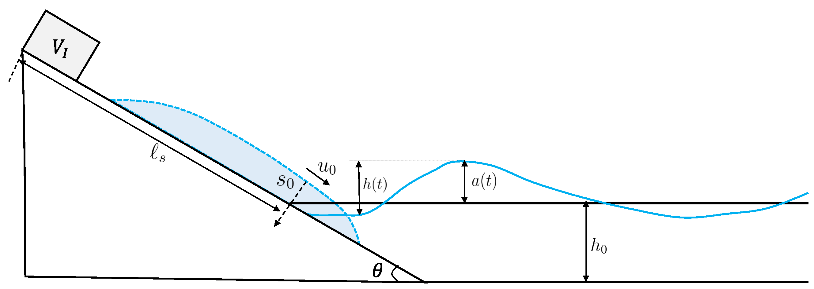
Figure 1. Sketch of the impacting process of landslide-generated waves.
Jmse 11 01151 g001
Figure 2. The three-dimensional structure of a data panel model.
Jmse 11 01151 g002
Figure 3. Sketch of the sliding mass (a) at rest and (b) moving along the slope.
Jmse 11 01151 g003
Figure 4. (a) Sketch of the facilities, (b) settings of the laser and lenses where I denotes a circular lens, II is a laser line generator lens, III is a rectangular lens, IV is an oblong lens, (c) is the raw image of the Carbopol observed by PIV, (d) is the raw image of water observed by PIV.
Jmse 11 01151 g004
Figure 5. Comparing (a) A m and (b) H m obtained from experimental measurements with the results predicted from empirical equations.
Jmse 11 01151 g005
Figure 6. Numerical solution of the depth-averaged velocity u ¯ ( x , t ) .
Jmse 11 01151 g006
Figure 7. Numerical solution of the slide thickness s ( x , t ) .
Jmse 11 01151 g007
Figure 8. Time evolution of (a) s 0 ( t ) and (b) u ¯ 0 ( t ) of the selected test.
Jmse 11 01151 g008
Figure 9. Time variation of (a) the wave amplitude a ( t ) and (b) the wave height h ( t ) .
Jmse 11 01151 g009
Figure 10. Classification results based on the evaluation criteria Fr, M, and S.
Jmse 11 01151 g010
Figure 11. Two-dimensional distributions of experiments in each class: (a) P and A m / H m , (b) A m / L m and H m / L m , (c) A m / L m and A m / H m .
Jmse 11 01151 g011
Figure 12. A ( T ) of the 10 validation tests, where N = 1 , 2 , , 10 denotes the test number. The black dots denote the experimental data and the red dots denote predicted data.
Jmse 11 01151 g012
Figure 13. Comparison of R T H E 2 and R E X P 2 of A ( T ) for the whole dataset.
Jmse 11 01151 g013
Table 1. Initial parameters of the selected tests, which serve as examples.
Testc [%] s [m] θ [-] m I [kg] h 0 [m]
T12.01.05 π / 4 3.00.2
T22.00.95 π / 4 3.50.2
T32.00.85 π / 4 4.00.2
T42.00.85 π / 4 4.50.2
Table 2. R 2 and MSE of A with the explanatory variables given by experimental results and theoretical approximations.
Nbr R EXP 2 MSE EXP R THE 2 MSE THE
10.9270.3270.8890.402
20.9340.2730.9240.292
30.9390.1960.8940.205
40.9280.4640.9140.506
50.9290.1350.9290.136
60.9311.4900.9051.549
80.8731.0480.8911.177
90.9370.6430.9300.680
100.9230.5430.9160.566
Disclaimer/Publisher’s Note: The statements, opinions and data contained in all publications are solely those of the individual author(s) and contributor(s) and not of MDPI and/or the editor(s). MDPI and/or the editor(s) disclaim responsibility for any injury to people or property resulting from any ideas, methods, instructions or products referred to in the content.