Analytical and Computational Modeling for Multi-Degree of Freedom Systems: Estimating the Likelihood of an FOWT Structural Failure

Abstract

Wind turbines and their associated parts are subjected to cyclical loads, such as bending, torque, longitudinal stresses, and twisting moments. The novel spatiotemporal reliability technique described in this research is especially useful for high-dimensional structural systems that are either measured or numerically simulated during representative observational time span. As this study demonstrates, it is possible to predict risks of dynamic system failure or damage given the in situ environmental load pattern. As an engineering example for this reliability, the authors have chosen 10-MW floating wind turbines and their dynamic responses, under environmental loadings, caused by wind and waves. The aim of this study was to benchmark a state-of-the-art approach suitable for the reliable study of offshore wind turbines. Existing reliability methods do not easily cope with dynamic system high dimensionality. The advocated reliability technique enables accurate and efficient assessment of dynamic system failure probability, accounting for system nonlinearities and high dimensionality as well as cross-correlations between different system components.

1. Introduction

As more offshore wind turbines have recently been developed, wind energy is taking lead in the field of renewable green energy. Wind energy is accessible, cost-free, and has great potential to be environmentally friendly. Installation of new, larger wind turbines has been relocated offshore due to available space and greater offshore wind potential [1]. No greenhouse gases, such as carbon dioxide, sulphur oxide, or nitrogen oxide, are released during the wind turbine’s operation. The contemporary market for floating (offshore) wind turbines (FWT, FOWT) has expanded along with a variety of accompanying technologies currently developed and already in use. According to the International Renewable Energy Agency (IRENA), offshore wind energy capacity will increase about 60% worldwide by 2050 [2]. In Europe, the Netherlands is leading, followed by UK, Belgium, and Germany. As offshore wind turbines have been further developed and newly put into service, there is a growing need to economically optimize the design of new turbines while maintaining their safety margins along with operational readiness levels. To minimize failures, improve design, and reduce maintenance downtime, accurate loads and structural reaction prediction methods are required to be used along with control algorithms, aerodynamics models, and dynamics of FOWTs.

Bottom-fixed monopile windfarms make up the majority of modern offshore windfarms. However, bottom-fixed wind turbines are not yet profitable [3]. About 80% of wind turbines are installed in deep seas, where floating offshore wind turbines (FOW) offer a considerable advantage. For an illustration of the various types of floating wind turbines, see Figure 1 up.

In the past two decades, the FWT size increased to save costs, and as its capacity increased, new technological developments were required for crucial parts including the motor, blades, and control. The majority of wind turbines, however, did not survive as long as they were expected to, which had negative effects on expenses. According to studies on wind turbine drivetrain status monitoring, the drivetrain gearbox failure may cause the highest downtime per repair [3,4,5]. For alternative approaches on the design of FOWTs as well as the current research status and future prospects, see [6,7,8,9,10,11]. As offshore wind industry improves designs, production, and deployment of big FWTs (10 MW and above), it should lead to even more refined designs and reduced failure rates within the next decade (see Figure 1). It would then be possible to build and execute a better FWT structural design and control system with the help of accurate and efficient calculations of FWT failure risks, [12,13,14,15,16,17,18,19,20,21,22].

To understand and develop numerical methods for estimating effects of waves and wind on wind turbines, several studies were carried out. Fatigue damage along with extreme structural responses of semi-submersible FOWTs were assessed in [5] while accounting for wave nonlinearities. The FWT drivetrain dynamics of a 750 KW spar type FWT was highlighted by [6,7,8]. Drivetrains for floating wind turbines have more complex load uncertainties than drivetrains for land-based turbines because of additional hydrodynamic effects. For future 10-MW FWT drivetrains, there is a pressing need to provide novel drivetrain design along with proper dynamic analysis. In Refs. [9,10,11], authors contributed to further developing of the 10-MW FWT design, modelling, and investigation of FWTs dynamic behavior. Hence, research on dynamic system resilience under high loads is critical for design of future low-risk operations. In addition, loads acting on FWTs exhibit stochastic behavior due to the wind action in terms of speed, direction, shear, and vorticity, thus necessitating rigorous load analysis throughout designed operational lifetime of wind turbine drivetrains. The methodology advocated in this study is based on structural dynamic models, aerodynamic models, and control algorithms. In this study, the SIMPACK (multibody simulation method) software tool was used to assess floating wind turbine drivetrains’ empirical bending moments.

To identify structural load reactions, proper understanding of the drivetrains’ dynamic behavior is required. This will allow us to decrease the failure rate, increase service life, and save costs. In the hydrodynamic study of FWTs, irregular waves and water depth are two separate concepts since FWTs are frequently placed in shallow-water areas where waves become more nonlinear and create a significant increase in hydrodynamic loads. One of two strategies may be used to evaluate extreme FWT loads. The first strategy is to simulate extreme events that lead to large structural loads. The second strategy, in contrast, simulates a wind turbine under normal operational conditions; the extreme probability distribution tail is then extrapolated [23,24,25,26,27,28,29,30].

2. Theoretical Background

The FWT drivetrain is decoupled in the two following steps. First, to identify in situ environmental loads and resulting stresses of the drivetrain, global aero-hydro-elastic-servo experiments in FAST (fatigue, aerodynamics, structures, and turbulence) is run. Following that, the loads and movements are employed as inputs in an SIMPACK multi-body drivetrain model. The gearbox’s feedback forces need to be minimized in an optimal way given the fact that the eigen-frequencies of the gearbox are substantially higher than those of the WT structure.

2.1. Hydro-Servo-Aero-Elastic Analysis Using FAST

FAST or Open FAST is the name of the engineering tool created by NREL to study the coupled dynamic response of FWT. To establish a time domain coupled nonlinear, aero-hydro-servo-elastic modelling, FAST employs aerodynamics and hydrodynamics models along with control electrical system (servo) models and structural (elastic) dynamics models. Lattice or tubular towers, solid or shaky hubs, upwind or downwind rotors, two- or three-blade horizontal axis FWT rotors, pitch and stall control, and rigid or unbalanced hubs may all be examined using the FAST program. Rotor blades and floating structures with aerodynamic and hydrodynamic stresses as well as FAST’s AeroDyn and HydroDyn modules are then connected to SIMPACK.

2.2. Hydrodynamics

Hydrodynamic loads acting on 10-MW FWT are evaluated using NREL HydroDyn simulation modules and time domain hydrodynamic modules coupled to SIMPACK in order to enable FWT’s aero-hydro-servo-elastic modelling. The Morrison equation, along with linear potential theory, were used to determine the wind turbine floater hydrodynamic stresses. WAMIT (WAMIT, Inc., Chestnut Hill, MA, USA, www.WAMIT.com (accessed on 1 January 2023)) was used to assess damping coefficients, extra mass, and first-order wave excitation load transfer functions. Semi-submersible floater hydrodynamic stresses were calculated using potential flow theory along with Morison’s drag term. WAMIT panel code computes hydrodynamic coefficients, such as extra mass as well as potential damping coefficients, and it computes first-order wave excitation load transfer functions in the frequency domain first in accordance with potential flow theory. The hydrodynamic coefficients are then transformed via convolution into time domain.

2.3. Structural Dynamics

Combined multi-body along with structural modal approach is taken into account by FAST software to account for FWT’s structural dynamics. The tower, blades, and driveshaft are regarded as flexible bodies, whereas the nacelle, hub, and floater are rigid bodies. The Rayleigh damping model was used to model structural damping. Resolving equations of motion produced by Kane’s technique for rigid–flexible-coupled systems were used to predict time domain dynamic structural responses [5].

2.4. Dynamics of Control System

The control system utilized in 10-MW FWT has two operating modes: (a) below-rated and (b) full-rated. In order to maximize power production, the generator’s torque–speed curve regulates the FWT rotor’s rotational speed, keeping an appropriate tip speed ratio within the below-rated region. In order to reduce structural stresses and keep the specified power output, a proportional-integral (PI) algorithm was utilized, regulating FWT blade pitch angle across the whole range of the motor’s rated power. The PI parameters obtained from a land-based reference wind turbine (RWT) were altered to prevent adverse damping effects.

2.5. Aerodynamics

Aerodynamic loads acting on FWT blades were assessed using blade element momentum (BEM) theory. The BEM technique combines a variety of complex modifications, including dynamic stall corrections, tip loss, hub loss, and skewed input. Prandtl adjustments were utilized to take into account FWT hub and blade tip losses brought on by the small number of blades. Glauert correction was used for induction factors. The skewed inflow adjustment was implemented in the Pitt and Peters model using dynamic stall adjustments in Beddoes–Leishman model. For more information about aerodynamic load calculations in the AeroDyn theory documentation, see (www.nrel.gov (accessed on 1 January 2023)) [1,2,3,4].

2.6. Multibody Simulation Using SIMPACK

Using the multi-body simulation (MBS) method, dynamics of FWT moving parts and distribution of loads and forces on the FWT mechanical system was investigated. Because FWT includes many moving elements, including the hub, main shaft, bearing, gearbox, etc., and because MBS is designed to address dynamic system behavior of linked bodies, it is ideally suited to handle dynamic reactions of FWT. It is made up of both rigid and flexible sections that are joined together by a variety of joints and other restraints. MBS is able to gauge and improve the behavior of multi-body simulations by solving motion equations. Usually, the bodies are joined by joints, which can either be a force or a stiffness element, limiting the motion of the bodies in relation to one another. SIMPACK is used for dynamic analysis and numerical modelling. Using the simulation analysis tool SIMPACK, one can accurately simulate nonlinear motions of FWTs and then predict dynamic behavior of its mechanical and mechatronic systems.

3. System Description

3.1. DTU 10-MW RWT

The powertrain design employed in this study was the DTU (Technical University of Denmark) 10-MW RWT. As a part of the Light Rotor project, DTU Wind Energy and Vestas Wind System developed the 10-MW RWT. To offer a design foundation for optimized 10+ MW FWTs, DTU launched the Light Rotor project. DTU 10-MW RWT, which was employed as a powertrain design for this study, was proposed by scaling the NREL 5 MW reference wind turbine (WT), which has a medium-speed motor and an efficient, lightweight rotor. The key design element for the 10-MW DTU is displayed in

Table 1. DTU-10-MW RWT design summary [13].

Description	Values
Rating	10 MW
Rotor orientation and its configuration	Upwind and 3 blades
Rotor and hub diameters	178.3 m, 5.6 m
FWT hub height	119 m
Cut-in, rated, and cut-out wind-speed	4.0 m/s, 11.4 m/s, 25.0 m/s
Cut-in, rated rotor speed	6.0 RPM, 9.6 RPM
FWT-rated tip speed	90 m/s
Overhang, shaft tilt, pre-cone	7.07 m, 5°, 2.5°
Rotor mass	229 tons (each blade ~41 tons)
FWT nacelle mass	446 tons
Tower mass	605 tons

and

Table 2. DTU-10-MW RWT drivetrain summary.

Parameters	Values
FWT gearbox ratio	1:50
Minimum rotor speed (rpm)	6.0
Rated rotor speed (rpm)	9.6
Rated generator speed (rpm)	480.0
Electrical generator efficiency	94.0
Generator inertia about high-speed shaft (kg·m2)	1500.5
Free–free rigid shaft torsion mode natural frequency	4.0
Free–fixed rigid shaft torsion mode natural frequency	0.6

.

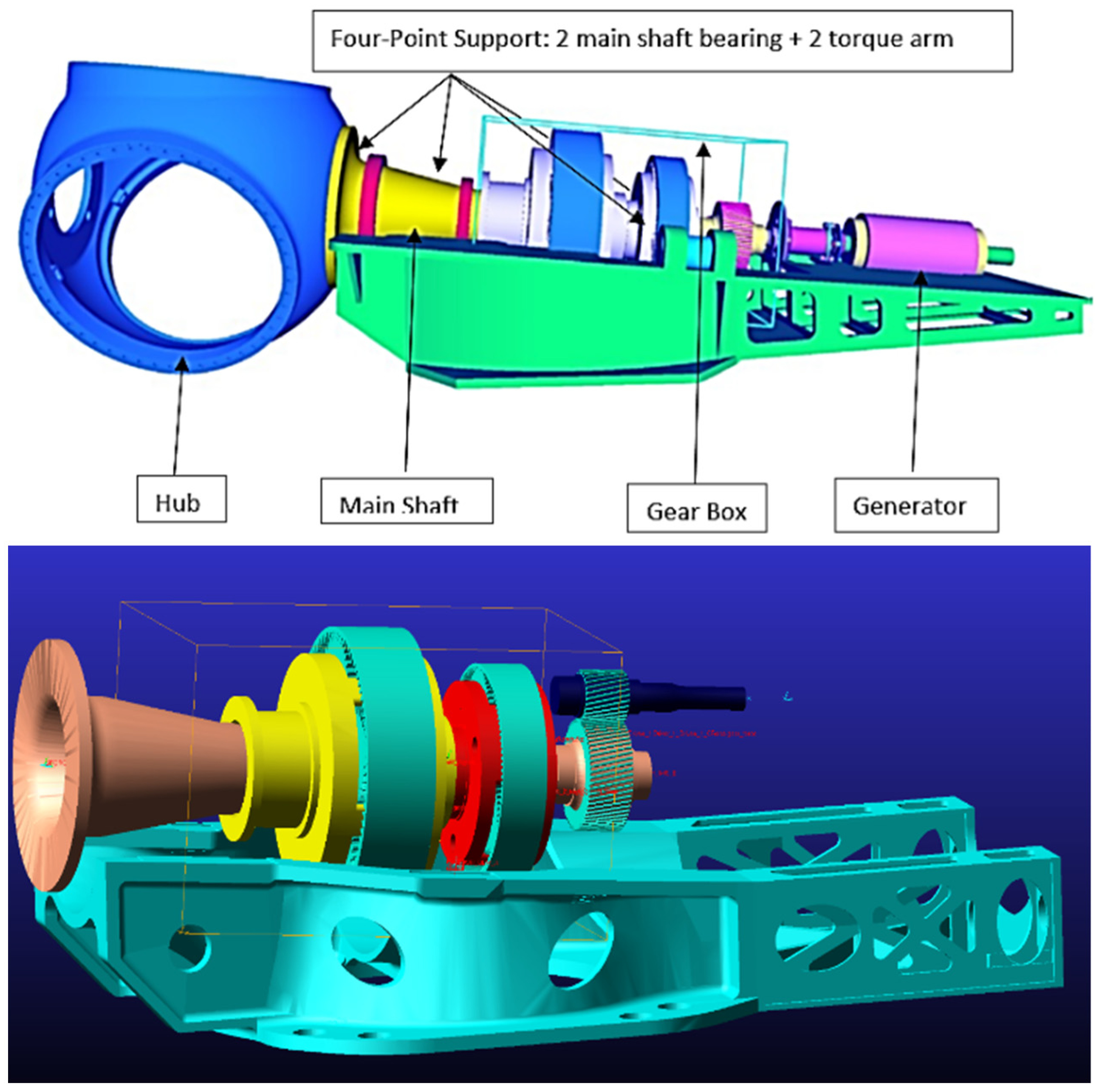
3.2. Drivetrain’s Design

The 10-MW powertrain was created in accordance with international standard IEC 61400-4 [8,9,10,11,12,13,14,15]. These standards address design specifications for FWT gearboxes and are applicable to horizontal-axis FWTs with a rating of more than 500 kW for onshore and offshore sectors. The drivetrain’s size and weight were kept to a minimum, while wind turbine efficiency was maximized by utilizing design foundation criteria that adhered with FLS and ULS specifications. The design notably minimized resonance, and logic of the new drivetrain model was compared to that of the DTU RWT that is now available. The 10-MW RWT optimal design resulted from continuous improvement in the numerical model of the driver train to satisfy FLS and ULS standards.

3.3. Drivetrain Layout

Based on industrial expertise, a four-point support system was employed with two main bearings on the main shaft and two bearings on the torque arm (Figure 2). This layout was chosen in light of research performed using a four-point support system, thus using with two main bearings on the main shaft and two bearings on the torque arm. The study conducted by [16] was focused on construction and use of main bearings in FWTs with a capacity of at least 10 MW. It was decided to use conventional three-stage gearbox, which comprises parallel and planetary stage gears. The three-stage gearbox consists of two planetary and one parallel stage gear. SIMPACK was used to generate a computational model of a 10-MW conventional powertrain and analyze its dynamics. The correctness and consistency of the numerical model were evaluated after the model was built in MBS and the characteristics of the drivetrain were explored [31,32,33].

The gear contact forces and bearing forces were calculated using the SIMPACK software, which can represent the entire dynamic conventional drivetrain model. The drivetrain was modelled as a spring and damper system with one degree of freedom, including joints and restrictions. Due to the fact that they were designed to handle forces, the bearings have six degrees of freedom. The model developed by [14] used first-order numerical eigenfrequency and yielded results less than 5% different from the theoretical model, illustrating the accuracy of the previously created drivetrain model.

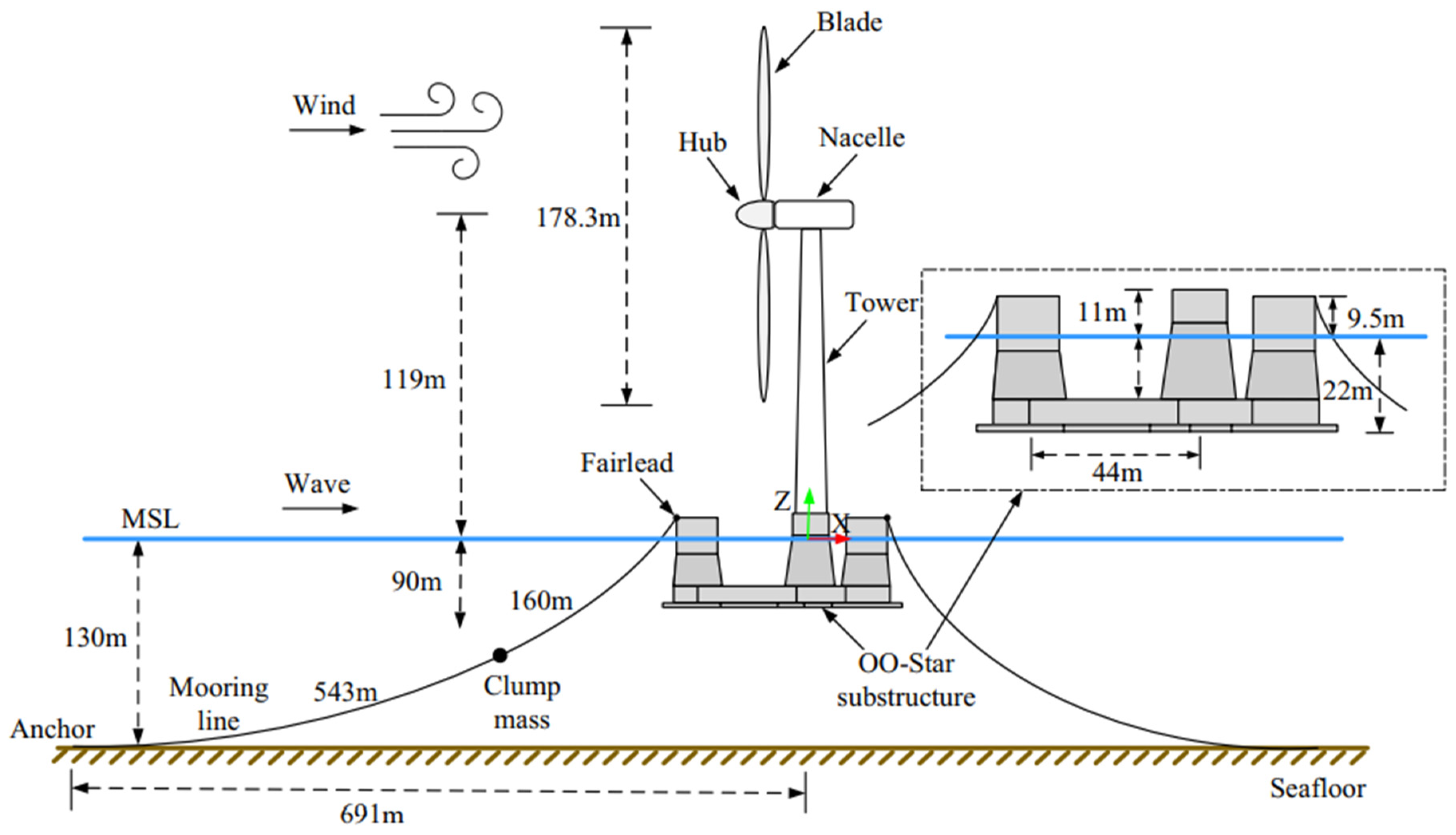
3.4. OO-Star Semi-Submersible FWT Floater with Mooring System

In the LIFES 50+ project, the semi-submersible floating substructure, supporting a 10-MW RWT was built [17]. A center column and three lateral columns with cylindrical top portions and tapering bottom sections each made up the floating substructure. The slab was linked at the FWT pontoon’s base, and the four columns were supported by a three-legged star-shaped pontoon (Figure 3).

3.5. Load Cases and Environmental Conditions

The Northern North Sea site’s [34] hindcast data measured between years 2010 and 2020 were used to generate the in situ wind–wave information that was utilized in this study. Based on in situ wind–wave data from the aforementioned site [34], the environmental parameters were identified, and combined wind–wave distribution was established taking into account 1 h mean wind speed at 10 m above the mean water level. (U₁₀) is the significant wave height (H_S), and the peak-period is (T_p)

$$f_{U_{10},H_S,T_p}\left(u,h,t\right)=f_{U_{10}}\left(u\right)·f_{H_S|U_{10}}\left(h|u\right)·f_{T_p|U_{10},H_S}\left(t|u,h\right)$$

(1)

In this study, three load examples were taken into account as the most common operational scenarios. The average operational wind speed is between 8 and 16 m/s (cut-in, rated, and cut-out). In general, wind turbines produce less power at speeds below 8 m/s than at speeds over 23 m/s, and they cease to a parked condition at speeds above 23 m/s to prevent mechanical damage.

Table 3. Numerical simulation of FWT load cases.

Load Cases	${\mathit{U}}_{\mathit{w}}(\mathbf{m}/\mathbf{s})$	${\mathit{T}}_{\mathit{I}}$	${\mathit{H}}_{\mathit{s}}\left(\mathbf{m}\right)$	${\mathit{T}}_{\mathit{p}}(\mathbf{s})$	Samples	Simulation Length (hours)
LC1	8	0.1740	1.9	9.7	24	1
LC2	12	0.1460	2.5	10.1	24	1
LC3	16	0.1320	3.2	10.7	24	1

describes three realistic load situations that were taken into consideration for this research and have a good chance of happening under ordinary in situ operational conditions. The mean wind speed utilized in this study was based on the operational ranges of FWTs, which vary between cut-in and cut-out zones that have a bin size of 4 m/s.

A straightforward wind-power law that is typically used to model vertical wind shear is as follows:

$$U\left(z\right)=U_{ref}{(\frac{Z}{Z_{ref}})}^{\alpha }$$

(2)

with

• U(z): Wind speed at the level z
• U_ref: Wind speed at the reference height
• Z_ref: Reference height
• α: Empirical wind–shear exponent

The power law exponent was α = 0.14 m for all wind speeds (see Table 3).

For operational scenarios, 10 random samples of wind–wave environmental sea states are normally utilized for each sea state, while severe wind and wave situations need the use of 24 random seeds of wind and wave. To create a simulation that lasts an hour, all simulations were run for 4000 s after deleting the 400 s starting transient phase.

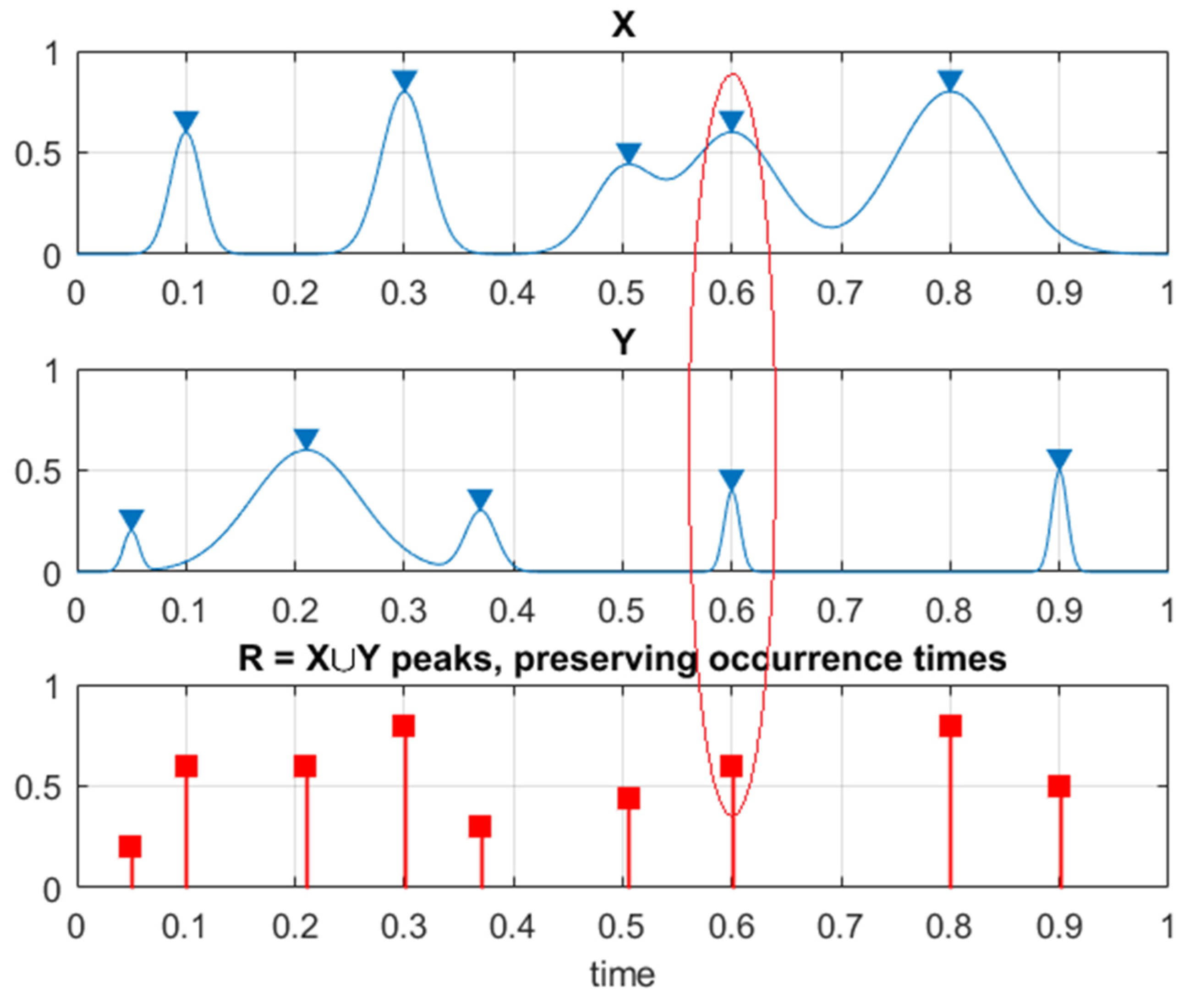
4. Novel Reliability Method

Ocean wind speeds are typically thought to follow a stationary, homogeneous ergodic random process. We must take into account an offshore multi-degree of freedom (MDOF) structure experiencing ergodic environmental loadings such as those brought on by the local wind–wave loads. An alternative is to think of a process as being dependent on ambient variables whose variation over time may be described as a separate ergodic process. Consider an MDOF structural response that is being jointly stationary. An example of a structural dynamic MDOF system is $\left(X\left(t\right), Y\left(t\right), Z\left(t\right), \dots \right)$ consisting of system’s vital components $X\left(t\right), Y\left(t\right), Z\left(t\right),\dots$ being simulated/measured/observed over a long enough (representative) time lapse $\left(0,T\right)$. Unidimensional system components’ global maxima during the whole lapse $\left(0,T\right)$ is denoted as $X_T^{\max }=\underset{0\le t\le T}{\max }X\left(t\right)$, $Y_T^{\max }=\underset{0\le t\le T}{\max }Y\left(t\right)$, $Z_T^{\max }=\underset{0\le t\le T}{\max }Z\left(t\right), \dots$ By long enough time lapse $T$, the authors primarily mean a large enough value of $T$ with respect to dynamic system relaxation and auto correlation times [35,36,37,38,39]. Let $X_1,\dots ,X_{N_X}$ be consequent in time the system component’s $X\left(t\right)$ local maxima, occurring at discrete time instants with monotonically rising rates $t_1^X<\dots <t_{N_X}^X$ in $\left(0,T\right)$. For more MDOF response components, the equivalent definition is as follows: $Y\left(t\right), Z\left(t\right), \dots$ with $Y_1,\dots ,Y_{N_Y};$ $Z_1,\dots ,Z_{N_Z}$ and so on. For convenience, all system components’ local maxima and components are considered to be non-negative. Estimating the likelihood of a system failure is the goal [40,41,42,43,44,45,46,47,48,49]

$$1-P=\mathrm{Prob}(X_T^{\max }>{\eta }_X {\displaystyle \cup } Y_T^{\max }>{\eta }_Y {\displaystyle \cup } Z_T^{\max }>{\eta }_Z {\displaystyle \cup } \dots )$$

(3)

with

$$P=\underset{\left(0, 0, 0, , \dots \right)}{\overset{\left({\eta }_X, {\eta }_Y, {\eta }_{Z }, \dots \right)}{{\displaystyle \iiint }}}{p}_{X_T^{\max }, Y_T^{\max }, Z_T^{\max } , \dots }\left(x_T^{\max }, y_T^{\max }, z_T^{\max }, \dots \right)d{x}_T^{\max }d{y}_T^{\max }d{z}_T^{\max }\dots$$

(4)

$P$ is the target non-exceedance probability that corresponds to critical system component values ${\eta }_X$, ${\eta }_Y$, ${\eta }_Z$, …; ${\displaystyle \cup }$ stands for logical unity operation «or»; and $p_{X_T^{\max }, Y_T^{\max }, Z_T^{\max } , \dots }$ is the overall joint PDF (probability density function) of system components’ global maxima within $\left(0,T\right)$. It is not practical, however, to explicitly estimate the latter joint probability distribution in reality $p_{X_T^{\max }, Y_T^{\max }, Z_T^{\max } , \dots }$ because of the low number of available data sets and high dimensionality. To put it another way, the moment when either $X\left(t\right)$ exceeds ${\eta }_X$, $Y\left(t\right)$ exceeds ${\eta }_Y$, $Z\left(t\right)$ exceeds ${\eta }_Z$, and so on, then the system is regarded as failed. Fixed system components hazard/failure levels ${\eta }_X$, ${\eta }_Y$, ${\eta }_Z$, … are individual for each system unidimensional system components $X_{N_X}^{\max }=\max \{X_j;j=1,\dots ,N_X\}=X_T^{\max }$, $Y_{N_Y}^{\max }=\max \{Y_j;j=1,\dots ,N_Y\}=Y_T^{\max }$, $Z_{N_z}^{\max }=\max \{Z_j;j=1,\dots ,N_Z\}=Z_T^{\max }$, and so on [50,51,52,53]. Local maxima time instants $\left[t_1^X<\dots <t_{N_X}^X;t_1^Y<\dots <t_{N_Y}^Y;t_1^Z<\dots <t_{N_Z}^Z\right]$ in monotonously non-decreasing order are sorted into one single merged temporal vector $t_1\le \dots \le t_N$. Note that $t_N=\max \{t_{N_X}^X, t_{N_Y}^Y, t_{N_Z}^Z, \dots \}$, $N\le N_X+N_Y+N_Z+\dots$. In this case $t_j$ represents system components’ local maxima of one of MDOF stationary system response components, being either $X\left(t\right)$, $Y\left(t\right)$, $Z\left(t\right)$, and so on. That means that having a dynamic system record time series, all that is required is to continually, concurrently search for system components’ local maxima within the system’s unidimensional response/load components and note when they surpass the MDOF hazard/limit system vector $\left({\eta }_X,{\eta }_Y,{\eta }_Z,\dots \right)$ in any of the system’s components $X, Y, Z, \dots$. A single temporally non-decreasing vector is created by combining the unidimensional system component’s local maxima $\overrightarrow{R}=\left(R_1, R_2, \dots ,R_N\right)$ in accordance with the merged temporal vector $t_1\le \dots \le t_N$. Every local maximum $R_j$ is actually an encountered component’s local maxima, corresponding to either system component $X\left(t\right)$, $Y\left(t\right)$, $Z\left(t\right)$, and so on. A unified system limit vector $\left({\eta }_1, \dots ,{\eta }_N\right)$ is now introduced with each component ${\eta }_j$ and is either ${\eta }_X$, ${\eta }_Y$, ${\eta }_Z$, and so on, depending on which of $X\left(t\right),$ $Y\left(t\right)$, $Z\left(t\right)$, etc. corresponds to the current local maxima with the running index $j$. Scaling parameter $0<\lambda \le 1$ are now implemented to artificially lower the limit/hazard values for all response/load components at the same time, namely new MDOF hazard/limit vector $\left({\eta }_X^{\lambda }, {\eta }_Y^{\lambda },{\eta }_z^{\lambda },\dots \right)$ with ${\eta }_X^{\lambda }\equiv \lambda ·{\eta }_X$, $\equiv \lambda ·{\eta }_Y$, ${\eta }_z^{\lambda }\equiv \lambda ·{\eta }_Z$, … being now introduced. A unified limit/hazard vector $\left({\eta }_1^{\lambda }, \dots , {\eta }_N^{\lambda }\right)$ is now introduced, having each its components ${\eta }_j^{\lambda }$ being equal to either ${\eta }_X^{\lambda }$, ${\eta }_Y^{\lambda }$, ${\eta }_z^{\lambda }$, etc. Hence, we have defined dynamic system survival probability $P\left(\lambda \right)$ as function of $\lambda$. Note that $P\equiv P\left(1\right)$ is from Equation (1). Non-exceedance system survival probability $P\left(\lambda \right)$ may be now estimated as follows [54,55,56,57,58,59,60,61,62,63,64]:

$$\begin{array}{l}P\left(\lambda \right)=\mathrm{Prob}\left\{R_N\le {\eta }_N^{\lambda },\dots ,R_1\le {\eta }_1^{\lambda }\right\}=\mathrm{Prob}\{R_N\le {\eta }_N^{\lambda } | R_{N-1}\le {\eta }_{N-1}^{\lambda },\dots ,R_1\\ \le {\eta }_1^{\lambda }\}\cdot \mathrm{Prob}\{R_{N-1}\le {\eta }_{N-1}^{\lambda },\dots ,R_1\le {\eta }_1^{\lambda }\}={\displaystyle \prod _{j=2}^N}\mathrm{Prob}\{R_j\le {\eta }_j^{\lambda } | R_{j-1}\\ \le {\eta }_{j-1}^{\lambda },\dots ,R_1\le {\eta }_1^{\lambda }\}\cdot \mathrm{Prob}\left(R_1\le {\eta }_1^{\lambda }\right)\end{array}$$

(5)

In offshore engineering practice, correlative dependency between the neighboring $R_j$ is not always readily negligible; hence, following one-step conditioning number $k=1$) memory approximation is now introduced

$$\mathrm{Prob}\{R_j\le {\eta }_j^{\lambda } | R_{j-1}\le {\eta }_{j-1}^{\lambda },\dots ,R_1\le {\eta }_1^{\lambda }\}\approx \mathrm{Prob}\{R_j\le {\eta }_j^{\lambda } | R_{j-1}\le {\eta }_{j-1}^{\lambda }\}$$

(6)

for $2\le j\le N$ (conditioning number $k=2$). The approximation introduced by Equation (4) can be further elaborated as

$$\mathrm{Prob}\{R_j\le {\eta }_j^{\lambda } | R_{j-1}\le {\eta }_{j-1}^{\lambda },\dots ,R_1\le {\eta }_1^{\lambda }\}\approx \mathrm{Prob}\{R_j\le {\eta }_j^{\lambda } | R_{j-1}\le {\eta }_{j-1}^{\lambda }, R_{j-2}\le {\eta }_{j-2}^{\lambda }\}$$

(7)

where $3\le j\le N$ conditioning number $k=3$), and so on. Monitoring each independent hazard/failure that occurred locally first in time is the goal in order to prevent cascade local intercorrelated exceedances. Statistical dependence effects between neighboring in time maxima can be captured more precisely with the latter type of approximations. The development of the stationary process was expected to be ergodic and stationary because of the MDOF dynamic system $p_k\left(\lambda \right)≔\mathrm{Prob}\{R_j>{\eta }_j^{\lambda } | R_{j-1}\le {\eta }_{j-1}^{\lambda }, R_{j-k+1}\le {\eta }_{j-k+1}^{\lambda }\}$ for $j\ge k$ will be independent on $j$ but only dependent on conditioning number $k$. Thus, non-exceedance (survival) probability may be now approximated as

$$P_k\left(\lambda \right)\approx \exp (-N·p_k\left(\lambda \right)) , k\ge 1$$

(8)

Equation (6) follows from Equation (1), if neglecting $\mathrm{Prob}\left(R_1\le {\eta }_1^{\lambda }\right)\approx 1$, as the risks of a design failure is low. In addition, it is expected that $N\gg k$. Note that Equation (5) is comparable to the well-known relationship between exceedance probability and the mean up-crossing rate function. Convergence with regard to conditioning parameter is observed for increasing $k$

$$P=\underset{k\to \infty }{\lim }{P}_k\left(1\right); p\left(\lambda \right)=\underset{k\to \infty }{\lim }{p}_k\left(\lambda \right)$$

(9)

Note that Equation (6) for $k=1$ becomes the well-known mean up-crossing rate function, related to non-exceedance (survival) probability

$$P\left(\lambda \right)\approx \exp (-{\nu }^{+}\left(\lambda \right)T); {\nu }^{+}\left(\lambda \right)={{\displaystyle \int }}_0^{\infty }\zeta p_{R\dot{R}}\left(\lambda ,\zeta \right)\zeta d\zeta$$

(10)

with $\zeta p_{R\dot{R}}$ being joint PDF, ${\nu }^{+}\left(\lambda \right)$ being mean up-crossing rate function of non-dimensional response level $\lambda$ for above-assembled non-dimensional vector $R\left(t\right)$ assembled from properly scaled MDOF dynamic system components $\left(\frac{X}{{\eta }_X}, \frac{Y}{{\eta }_Y}, \frac{Z}{{\eta }_Z}, \dots \right)$, see Figure 4.

Note that a stationarity premise was used above. The provided technique can also be used to manage non-stationary cases. An example that follows shows how the method can be used in non-stationary situations. Given a scatter diagram, consisting of $m=1,\dots ,M$ environmental states, each short-term environmental sea state has probability $q_m$, such that ${{\displaystyle \sum }}_{m=1}^M{q}_m=1$. The corresponding long-term equation is then

$$p_k\left(\lambda \right)\equiv {\displaystyle \sum }_{m=1}^M{p}_k\left(\lambda ,m\right)q_m$$

(11)

with $p_k\left(\lambda ,m\right)$ being the same function as in Equation (7) but with the number matching the particular in situ short-term environmental condition $m$. The above-presented $p_k\left(\lambda \right)$ functions are often regular in their tail, i.e., for extreme values of $\lambda$ approaching extreme level $1$. More precisely, for $\lambda \ge {\lambda }_0$, the distribution tail behaves like $\exp \left\{-{\left(a\lambda +b\right)}^c+d\right\}$ with $a, b, c, d$ being four fitted constants for the appropriate tail cut-on ${\lambda }_0$ value. Optimal values of $a, b, c, \mathrm{and} d$ may be determined using a sequential quadratic programming (SQP) technique, implemented in NAG Numerical Library.

5. Failure Probability Estimation

This section illustrates how the advocated methodology may be used in engineering practice. Internal stresses and bending moments of 14 crucial gearbox bearings were selected as components $X, Y, Z, \dots ,$ hence constituting an example of a fourteen-dimensional (14D) system. FWT numerical simulation has been done for a range of different realistic wind speeds; in total, 20 independent 1 h response time series were generated for each wind speed, and the discrete time step was $dt=0.025$ s. For simplicity, the global maximum of each unidimensional component force was increased by 50% to represent a critical threshold, causing FWT to fail. In order to unify all 14 measured time series $X, Y, Z$, … the following scaling was conducted:

$$X\to \frac{X}{{\eta }_X}, Y\to \frac{Y}{{\eta }_Y}, Z\to \frac{Z}{{\eta }_Z}, \dots$$

(12)

making all 14 responses non-dimensional and having the same failure/hazard limits simultaneously equal to 1. Then, by maintaining them in a temporal non-decreasing order, all local maxima from the 14 recorded time series were combined into one merged time series: $R\left(t\right)\equiv \overrightarrow{R}=\left(\max \left\{X_1,Y_1,Z_1,\dots \right\},\dots ,\max \left\{X_N,Y_N,Z_{N,\dots }\right\}, \dots \right)$ with each set $\max \left\{X_j,Y_j,Z_j, \dots \right\}$ being ranked based on the non-decreasing occurrence times of these local maxima [59,60,61,62,63,64,65].

Figure 5 presents an example of a non-dimensional assembled vector $\overrightarrow{R}$, consisting of assembled local maxima of the FWT’s internal forces; $\lambda >0.05$ cut-on limit was used for illustrative purposes, as lower values $\lambda \ge 0$ are obviously irrelevant for the failure/hazard system’s PDF tail extrapolation towards the target $\lambda =1$. Note that system vector $\overrightarrow{R}$ does not have any physical meaning on its own, as it was assembled from different system components having different measurement units (MPa and Nm in our case). The index $j$ is just the running index of local maxima, encountered in a non-decreasing time sequence.

Figure 6 presents an extrapolation (solid line) according to Equation (9) towards hazard/failure state, which is 1 and somewhat beyond. The $\lambda =0.25$ cut-on value was used. Dotted lines indicate extrapolated 95% confidence intervals (CI). According to Equation (5), $p\left(\lambda \right)$ is directly related to the target system failure probability $1-P$ from Equation (1). Therefore, in agreement with Equation (5), system failure probability $1-P\approx 1-P_k\left(1\right)$ can be now estimated. Note that in Equation (5), $N$ corresponds to the total number of local maxima within the unified system vector $\overrightarrow{R}$. The conditioning number $k=6$ was found to be sufficient due to convergence occurrence with respect to $k$ (see Equation (6)). Figure 6 exhibits a relatively narrow 95% CI.

Note that discretization of the equations and the order or accuracy of the chosen discretization scheme were not discussed in this study. Sensitivity analysis to evaluate the sensitivity of the output to changes in input parameters was left for future studies. Incorporating sensitivity analysis is critical to assess robustness and reliability of the model’s predictions. Neglecting parameter sensitivity could result in inadequate capturing of uncertainties and variations in the system. The latter was due to the fact that this study was focused primarily on demonstration of a novel reliability technique and not much on the underlying numerical model itself.

6. Conclusions

This study examined simulated response time series of offshore floating wind turbines. Application of a novel spatiotemporal reliability method to multidimensional wind energy system reliability was conducted, the theoretical rationale of the proposed technique was discussed.

The goal of this study was to develop a general-purpose, yet reliable and easy-to-use multi-dimensional reliability technique. As seen from the results, the suggested method produced fairly narrow confidence intervals. The suggested method might therefore be used for a variety of nonlinear dynamic system reliability studies, especially at the design stage. Both measured and numerically simulated dynamic system responses may be used as an underlying dataset.

As this study demonstrates, it is feasible to accurately assess risks of complex system failure or damage, while efficiently utilizing available datasets. To summarize, the suggested method can be applied to various engineering and design applications. The engineering system considered in this study by no means limits applicability of the suggested reliability methodology.

Note that stability properties are critical for the numerical methods employed in the structural model. Failing to analyze and consider stability, particularly for methods such as explicit time integration schemes, can lead to inaccurate or divergent solutions. Ensuring the stability of the numerical methods is crucial for reliable and meaningful results.

Among potential limitations of suggested methodology is that the underlying dataset should be representative and filtered from outliers; another major requirement is system stationarity. In cases where an underlying trend is present, it is necessary to identify this trend first.

References

1. International Energy Agency. World Energy Outlook 2020; OECD Publishing: Paris, France, 2020. [Google Scholar]
2. Veers, P.; Butterfield, S. Extreme load estimation for wind turbines-issues and opportunities for improved practice. In Proceedings of the 20th 2001 ASME Wind Energy Symposium, Reno, NV, USA, 11–14 January 2001; p. 44. [Google Scholar]
3. Igba, J.; Alemzadeh, K.; Durugbo, C.; Henningsen, K. Performance assessment of wind turbine gearboxes using in-service data: Current approaches and future trends. Renew. Sustain. Energy Rev. 2015, 50, 144–159. [Google Scholar] [CrossRef] [Green Version]
4. International Renewable Energy Agency (IRENA). Renewable Energy Technologies: Cost Analysis Series. Wind Power; IRENA: Abu Dhabi, United Arab Emirates, 2012. [Google Scholar]
5. Sheng, S. Wind Turbine Gearbox Condition Monitoring Round Robin Study-Vibration Analysis; No. NREL/TP-5000-54530; National Renewable Energy Laboratory (NREL): Golden, CO, USA, 2012.
6. O’Kelly, B.C.; Arshad, M. Offshore wind turbine foundations—Analysis and design. In Offshore Wind Farms; Woodhead Publishing: Sawston, UK, 2016; pp. 589–610. [Google Scholar]
7. Barooni, M.; Ashuri, T.; Velioglu Sogut, D.; Wood, S.; Ghaderpour Taleghani, S. Floating Offshore Wind Turbines: Current Status and Future Prospects. Energies 2022, 16, 2. [Google Scholar] [CrossRef]
8. Veers, P.S.; Winterstein, S.R. Application of measured loads to wind turbine fatigue and reliability analysis. J. Sol. Energy Eng. 1998, 120, 233–239. [Google Scholar] [CrossRef] [Green Version]
9. Dimitrov, N. Comparative analysis of methods for modelling the short-term probability distribution of extreme wind turbine loads. Wind Energy 2016, 19, 717–737. [Google Scholar] [CrossRef]
10. Madsen, P.; Pierce, K.; Buhl, M. Predicting ultimate loads for wind turbine design. In Proceedings of the 37th Aerospace Sciences Meeting and Exhibit, Reno, NV, USA, 11–14 January 1999; p. 69. [Google Scholar]
11. Ronold, K.O.; Wedel-Heinen, J.; Christensen, C.J. Reliability-based fatigue design of wind-turbine rotor blades. Eng. Struct. 1999, 21, 1101–1114. [Google Scholar] [CrossRef]
12. Ronold, K.O.; Larsen, G.C. Reliability-based design of wind-turbine rotor blades against failure in ultimate loading. Eng. Struct. 2000, 22, 565–574. [Google Scholar] [CrossRef]
13. Manuel, L.; Veers, P.S.; Winterstein, S.R. Parametric models for estimating wind turbine fatigue loads for design. J. Sol. Energy Eng. 2001, 123, 346–355. [Google Scholar] [CrossRef] [Green Version]
14. Fitzwater, L.M.; Cornell, A.C. Predicting the long term distribution of extreme loads from limited duration data: Comparing full integration and approximate methods. J. Sol. Energy Eng. 2002, 124, 378–386. [Google Scholar] [CrossRef]
15. Moriarty, P.J.; Holley, W.E.; Butterfield, S. Effect of turbulence variation on extreme loads prediction for wind turbines. J. Sol. Energy Eng. 2002, 124, 387–395. [Google Scholar] [CrossRef]
16. Agarwal, P.; Manuel, L. Extreme loads for an offshore wind turbine using statistical extrapolation from limited field data. Wind. Energy Int. J. Prog. Appl. Wind Power Convers. Technol. 2008, 11, 673–684. [Google Scholar] [CrossRef] [Green Version]
17. Barreto, D.; Karimirad, M.; Ortega, A. Effects of Simulation Length and Flexible Foundation on Long-Term Response Extrapolation of a Bottom-Fixed Offshore Wind Turbine. J. Offshore Mech. Arct. Eng. 2022, 144, 032001. [Google Scholar] [CrossRef]
18. McCluskey, C.J.; Guers, M.J.; Conlon, S.C. Minimum sample size for extreme value statistics of flow-induced response. Mar. Struct. 2021, 79, 103048. [Google Scholar] [CrossRef]
19. Fogle, J.; Agarwal, P.; Manuel, L. Towards an improved understanding of statistical extrapolation for wind turbine extreme loads. Wind. Energy Int. J. Prog. Appl. Wind Power Convers. Technol. 2008, 11, 613–635. [Google Scholar]
20. Ernst, B.; Seume, J.R. Investigation of site-specific wind field parameters and their effect on loads of offshore wind turbines. Energies 2012, 5, 3835–3855. [Google Scholar] [CrossRef] [Green Version]
21. Graf, P.A.; Stewart, G.; Lackner, M.; Dykes, K.; Veers, P. High-throughput computation and the applicability of Monte Carlo integration in fatigue load estimation of floating offshore wind turbines. Wind Energy 2016, 19, 861–872. [Google Scholar] [CrossRef]
22. Fitzwater, L.M.; Winterstein, S.R. Predicting design wind turbine loads from limited data: Comparing random process and random peak models. J. Sol. Energy Eng. 2001, 123, 364–371. [Google Scholar] [CrossRef] [Green Version]
23. Moriarty, P.J.; Holley, W.E.; Butterfield, S.P. Extrapolation of Extreme and Fatigue Loads Using Probabilistic Methods; No. NREL/TP-500-34421; National Renewable Energy Laboartory (NREL): Golden, CO, USA, 2004.
24. Freudenreich, K.; Argyriadis, K. The load level of modern wind turbines according to IEC 61400-1. J. Phys. Conf. Ser. 2007, 75, 012075. [Google Scholar] [CrossRef]
25. Ragan, P.; Manuel, L. Statistical extrapolation methods for estimating wind turbine extreme loads. J. Sol. Energy Eng. 2008, 130, 031011. [Google Scholar] [CrossRef]
26. Peeringa, J.M. Comparison of Extreme Load Extrapolations Using Measured and Calculated Loads of a MW Wind Turbine; ECN: Petten, The Netherlands, 2009. [Google Scholar]
27. Abdallah, I. Assessment of Extreme Design Loads for Modern Wind Turbines Using the Probabilistic Approach. Ph.D. Thesis, Technical University of Denmark, Roskilde, Denmark, 2015. [Google Scholar]
28. Stewart, G.M.; Lackner, M.A.; Arwade, S.R.; Hallowell, S.; Myers, A.T. Statistical Estimation of Extreme Loads for the Design of Offshore Wind Turbines During Non-Operational Conditions. Wind Eng. 2015, 39, 629–640. [Google Scholar] [CrossRef]
29. Gaidai, O.; Wang, F.; Wu, Y.; Xing, Y.; Medina, A.; Wang, J. Offshore renewable energy site correlated wind-wave statistics. Probabilistic Eng. Mech. 2022, 68, 103207. [Google Scholar] [CrossRef]
30. Gaidai, O.; Storhaug, G.; Næss, A. Statistics of extreme hydroelastic response for large ships. Mar. Struct. 2019, 61, 142–154. [Google Scholar] [CrossRef]
31. Xu, X.; Xing, Y.; Gaidai, O.; Wang, K.; Patel, K.; Dou, P.; Zhang, Z. A novel multi-dimensional reliability approach for floating wind turbines under power production conditions. Front. Mar. Sci. 2022, 9, 970081. [Google Scholar] [CrossRef]
32. Gaidai, O.; Xing, Y.; Balakrishna, R. Improving extreme response prediction of a subsea shuttle tanker hovering in ocean current using an alternative highly correlated response signal. Results Eng. 2022, 15, 100593. [Google Scholar] [CrossRef]
33. Cheng, Y.; Gaidai, O.; Yurchenko, D.; Xu, X.; Gao, S. Study on the Dynamics of a Payload Influence in the Polar Ship. In Proceedings of the 32nd International Ocean and Polar Engineering Conference, Shanghai, China, 6–10 June 2022. Paper Number ISOPE-I-22-342. [Google Scholar]
34. Available online: https://seklima.met.no/ (accessed on 1 January 2023).
35. Gaidai, O.; Fu, S.; Xing, Y. Novel reliability method for multidimensional nonlinear dynamic systems. Mar. Struct. 2022, 86, 103278. [Google Scholar] [CrossRef]
36. Gaidai, O.; Yan, P.; Xing, Y. A novel method for prediction of extreme wind speeds across parts of Southern Norway. Front. Environ. Sci. 2022, 10, 997216. [Google Scholar] [CrossRef]
37. Gaidai, O.; Yan, P.; Xing, Y. Prediction of extreme cargo ship panel stresses by using deconvolution. Front. Mech. Eng. 2022, 8, 992177. [Google Scholar] [CrossRef]
38. Falzarano, J.; Su, Z.; Jamnongpipatkul, A. Application of stochastic dynamical system to nonlinear ship rolling problems. In Proceedings of the 11th International Conference on the Stability of Ships and Ocean Vehicles, Athens, Greece, 23–28 September 2012. [Google Scholar]
39. Gaidai, O.; Xu, J.; Yan, P.; Xing, Y.; Zhang, F.; Wu, Y. Novel methods for wind speeds prediction across multiple locations. Sci. Rep. 2022, 12, 19614. [Google Scholar] [CrossRef]
40. Gaidai, O.; Xing, Y. Novel reliability method validation for offshore structural dynamic response. Ocean Eng. 2022, 266, 113016. [Google Scholar] [CrossRef]
41. Gaidai, O.; Wu, Y.; Yegorov, I.; Alevras, P.; Wang, J.; Yurchenko, D. Improving performance of a nonlinear absorber applied to a variable length pendulum using surrogate optimization. J. Vib. Control 2022, 10775463221142663. [Google Scholar] [CrossRef]
42. Gaidai, O.; Wang, K.; Wang, F.; Xing, Y.; Yan, P. Cargo ship aft panel stresses prediction by deconvolution. Mar. Struct. 2022, 88, 103359. [Google Scholar] [CrossRef]
43. Gaidai, O.; Xu, J.; Xing, Y.; Hu, Q.; Storhaug, G.; Xu, X.; Sun, J. Cargo vessel coupled deck panel stresses reliability study. Ocean Eng. 2023, 268, 113318. [Google Scholar] [CrossRef]
44. Gaidai, O.; Xing, Y. A Novel Multi Regional Reliability Method for COVID-19 Death Forecast. Eng. Sci. 2022, 21, 799. [Google Scholar] [CrossRef]
45. Gaidai, O.; Xing, Y. A novel bio-system reliability approach for multi-state COVID-19 epidemic forecast. Eng. Sci. 2022, 21, 797. [Google Scholar] [CrossRef]
46. Gaidai, O.; Yan, P.; Xing, Y. Future world cancer death rate prediction. Sci. Rep. 2023, 13, 303. [Google Scholar] [CrossRef] [PubMed]
47. Gaidai, O.; Xu, J.; Hu, Q.; Xing, Y.; Zhang, F. Offshore tethered platform springing response statistics. Sci. Rep. 2022, 12, 21182. [Google Scholar] [CrossRef]
48. Gaidai, O.; Xing, Y.; Xu, X. Novel methods for coupled prediction of extreme wind speeds and wave heights. Sci. Rep. 2023, 13, 1119. [Google Scholar] [CrossRef]
49. Gaidai, O.; Cao, Y.; Xing, Y.; Wang, J. Piezoelectric Energy Harvester Response Statistics. Micromachines 2023, 14, 271. [Google Scholar] [CrossRef]
50. Gaidai, O.; Cao, Y.; Loginov, S. Global cardiovascular diseases death rate prediction. Curr. Probl. Cardiol. 2023, 48, 101622. [Google Scholar] [CrossRef]
51. Gaidai, O.; Cao, Y.; Xing, Y.; Balakrishna, R. Extreme springing response statistics of a tethered platform by deconvolution. Int. J. Nav. Archit. Ocean Eng. 2023, 15, 100515. [Google Scholar] [CrossRef]
52. Gaidai, O.; Xing, Y.; Balakrishna, R.; Xu, J. Improving extreme offshore wind speed prediction by using deconvolution. Heliyon 2023, 9, e13533. [Google Scholar] [CrossRef]
53. Gaidai, O.; Xing, Y. Prediction of death rates for cardiovascular diseases and cancers. Cancer Innov. 2023, 2, 140–147. [Google Scholar] [CrossRef]
54. Xu, Y.; Øiseth, O.; Moan, T.; Naess, A. Prediction of long-term extreme load effects due to wave and wind actions for cable-supported bridges with floating pylons. Eng. Struct. 2018, 172, 321–333. [Google Scholar] [CrossRef]
55. Gaspar, B.; Naess, A.; Leira, B.; Soares, C. System reliability analysis of a stiffened panel under combined uniaxial compression and lateral pressure loads. Struct. Saf. 2012, 39, 30–43. [Google Scholar] [CrossRef]
56. Naess, A.; Stansberg, C.; Gaidai, O.; Baarholm, R. Statistics of extreme events in airgap measurements. J. Offshore Mech. Arct. Eng. 2009, 131, 733–742. [Google Scholar] [CrossRef]
57. Xu, X.; Gaidai, O.; Yakimov, V.; Xing, Y.; Wang, F. FPSO offloading operational safety study by a multidimensional reliability method. Ocean Eng. 2023, 281, 114652. [Google Scholar] [CrossRef]
58. Gaidai, O.; Xing, Y. COVID-19 Epidemic Forecast in Brazil. Bioinform. Biol. Insights 2023, 17, 11779322231161939. [Google Scholar] [CrossRef]
59. Gaidai, O.; Wang, F.; Xing, Y.; Balakrishna, R. Novel Reliability Method Validation for Floating Wind Turbines. Adv. Energy Sustain. Res. 2023, 2200177. [Google Scholar] [CrossRef]
60. Gaidai, O.; Hu, Q.; Xu, J.; Wang, F.; Cao, Y. Carbon Storage Tanker Lifetime Assessment. Glob. Chall. 2023, 2300011. [Google Scholar] [CrossRef]
61. Liu, Z.; Gaidai, O.; Xing, Y.; Sun, J. Deconvolution approach for floating wind turbines. Energy Sci. Eng. 2023, 1–9. [Google Scholar] [CrossRef]
62. Gaidai, O.; Yurchenko, D.; Ye, R.; Xu, X.; Wang, J. Offshore crane non-linear stochastic response: Novel design and extreme response by a path integration. Ships Offshore Struct. 2022, 17, 1294–1300. [Google Scholar] [CrossRef]
63. Gaidai, O.; Yan, P.; Xing, Y.; Xu, J.; Zhang, F.; Wu, Y. Oil tanker under ice loadings. Sci. Rep. 2023, 13, 8670. [Google Scholar] [CrossRef]
64. Gaidai, O.; Xing, Y.; Xu, J.; Balakrishna, R. Gaidai-Xing reliability method validation for 10-MW floating wind turbines. Sci. Rep. 2023, 13, 8691. [Google Scholar] [CrossRef] [PubMed]
65. Naess, A.; Gaidai, O.; Teigen, P. Extreme response prediction for nonlinear floating offshore structures by Monte Carlo simulation. Appl. Ocean. Res. 2007, 29, 221–230. [Google Scholar] [CrossRef]
Figure 1. (Up): The evolution of FWTs. (Down): Reliability and downtime in FWT sub-assemblies [3].
Jmse 11 01237 g001
Figure 2. (Up): Four-point support FWT configuration gearbox. (Down): 10-MW FWT drivetrain design in MBS software [32].
Jmse 11 01237 g002
Figure 3. OO-Star FWT wind floater’s semi-10-MW concept [31].
Jmse 11 01237 g003
Figure 4. Illustration on how two system component processes X and Y are combined into one new synthetic vector R. The red ellipse highlights a case of simultaneous maxima for different system components.
Jmse 11 01237 g004
Figure 5. Non-dimensional assembled 14D vector R example.
Jmse 11 01237 g005
Figure 6. Extrapolation of p k ( λ ) (on the y-axis) towards the critical level (marked by star) and beyond, conditioning index k = 6 . Extrapolated 95% CI marked by dotted lines. Horizontal x-axis corresponds to the non-dimensional parameter λ .
Jmse 11 01237 g006