Abstract
Animal population abundance is a significant parameter for studies on invasive species that can threaten the ecosystem. Researchers have been developing population estimation methods since the 18th century, in order to evaluate species’ evolution and environmental effects. However, studies on the population density of the invasive species Callinectes sapidus are very limited. The present work, using a simulation model combined with field measurements, examines an innovative methodology for estimating the current population of the invasive species Callinectes sapidus in a shallow Mediterranean coastal lagoon. The methodology presented here builds the first stage of modeling and predicting the evolution of this species’ population in marine environments. The simulation model’s results are validated with an estimation of the total population based on juvenile abundance, and a curvature of the species population estimation based on cage catch is implemented. The simulation experiments presented here show the possibility of a robust prediction for blue crab population estimation.
1. Introduction
Animal population evolution is critical for studies on invasive species that can threaten the ecosystem’s balance. Knowledge of species population densities is highly important to evaluate its evolution and effect on the ecosystem as well as to take proper measurements to prevent negative effects on other species. In terms of the commercial exploitation of a species, continuous knowledge of its population density is very significant in order to balance fishing rates and maintain the population density at certain levels (Even in the case of an invasive species, the local authorities may want to keep its density to a certain level for exploitation if found that it does not harm the local ecosystem). Therefore, it is important to continue to reinforce actions studying species dynamics, which could only begin by estimating the current population density of the species.
1.1. Animal Population Estimation Methods
Population estimation methods date back to the 18th century and are still evolving. The methods are categorized into direct sampling and indirect sampling methods. Direct sampling methods involve the counting of individuals, while indirect sampling methods involve the use of animal signs as indices of an individual’s presence, used for estimating animal density [1].
Some direct methods include drive counts [2,3,4,5], road counts, field strip counts [6,7,8], aerial counts [9,10], water hole counts [11], and line transects [12,13,14,15]. However, the flaw of these methods is that they are considered invasive for both the local vegetation and animal individuals and are subject to several assumptions [3,5,12,14,16,17,18,19,20,21].
When direct sampling methods are inaccurate due to the behavior of individuals and habitat preferences, indirect sampling methods are used. The main indirect sampling methods are pellet (dung) counts [2,3,7,12], track counts [4,5,13], and territorial marking (scrapes or rubs) counts [5]. Differences in habitat use, mobility, and defecation rates are some of the sources of uncertainties regarding the use of pellet counts [22]. Track and trackway counts can only be used as an indicator of animal presence and are not useful for population estimation [5].
Acoustic methods have been developed for estimating fish abundance [23,24,25,26,27,28,29,30]. Acoustic methods are suitable for large (and difficult to sample) areas such as underwater or dense forests. An issue with echo-sounding is the standardization of readings for converting relative densities to absolute densities. Difficulties also arise to evaluate species of fish from echo-sounding readings and the accuracy of the estimates for animal densities is affected by foraging sounds (sounds from different species or other sources tangled up with the studied species) and the sound level emitted by individuals (as differences in the decibel readings might indicate different species but this is not always clear) [31].
The removal method assumes constant sighting probabilities by observers in the field. Thus, the method is vulnerable to the heterogeneity of sighting between different observers and locations [32]. Removal models have also been proven to be biased when sample sizes are low [33].
The Lincoln–Petersen Model is one of the oldest models that date back to Laplace [34] and was first used for fisheries and wildlife estimations by Lincoln [35], White [36]. The assumptions of this model are that no individuals are added to or deleted from the population, all individuals have the same probability of getting caught and all marks are detected [37]. The Jolly–Seber model [38,39,40] is subject to the same assumptions as the Petersen model and assumes that marked individuals have the same probability of survival until the following sampling time as non-marked individuals.
Mark-recapture estimates of animal density have been proven unbiased but imprecise, and their performance drops at high or low animal densities [41]. Distance sampling methods (group of methods, which estimate the absolute density of a population based on the observer to animal distance [42]) were unbiased (with assumptions) but also imprecise [41]. Non-invasive genetic mark-recapture methods were highly biased compared to camera trap mark-recapture methods [43] (and expensive [44]). Additionally, the processing of the data (genetic samples or photo evaluation) is time-consuming [45].
Camera traps have been used combined with mark-recapture methods to estimate animal abundance from photographs and videos of recognizable species [46,47,48]. The recognizability of animal species is very significant, because otherwise the estimation occurs with the use of relative abundance methods, which have been criticized as biased and imprecise [49]. Nevertheless, depending on the area and animal population, these methods can be very expensive.
One of the latest methods developed for estimating animal densities is the random encounter model (REM) [50]. The REM’s assumptions are that animal movement is random and independent of each other and uses a constant speed (or distance travelled in 24 h) for animal movement detected by camera traps [51]. The disadvantages of this method are intensive labor and high costs in the field as well as the difficulty in estimating the daily travel distance of individual animals. Thus, only a few studies have been conducted using the REM model [52,53,54,55,56,57,58,59,60]. Therefore, a more efficient approach is highly needed.
An improvement to the RE model is the random encounter and staying time model (REST) described by Nakashima et al. [61]. Based on the REM model, REST uses video-recording cameras to estimate the staying time of animals within an area and uses them to estimate the animal movement speed without animal individual recognition. The authors used random walk movements to evaluate the model’s performance. However, there are four crucial assumptions associated with the REST model. These assumptions are that camera traps detect all individuals within an area and these individual species are identified, camera traps do not alter the movement or behavior of animals, the population density is constant during the survey, and camera traps are randomly placed within the area of a certain population. This new model has been recently used in ungulate density estimations [62]. Nevertheless, to account for its feasibility and applicability more studies are required [63].
1.2. Challenges in Estimating Population Abundance in Aquatic Environments
All the aforementioned methods in estimating species abundance can be applied in all kinds of terrestrial environments from deserts to dense forests. However, when the studied species thrive in aquatic environments, evaluating their abundance can be more complex. More specifically, many methods rely on aerial and ground surveys as well as measurements using cameras. This is not always easy underwater, as the turbidity of the water can affect its clarity resulting in the identification and count of species being biased (multiple counts of the same individuals) and/or impossible due to the heterogeneity of sight ability in the measurements [32]. Another issue with underwater measurements is that catchability may vary for a lot of reasons (e.g., gear saturation) and this is not always detected as traps and nets cannot be seen from a distance without removing them from the study site [64]. Moreover, one of the greatest differences between terrestrial and aquatic species is that in the aquatic environment, most species move in three dimensions. Thus, remote detectors (often used in mark-recapture studies) need to adapt to different monitoring setups and use capture-frequency data [65]. All these emerging difficulties in studying aquatic species render the selected methods time-consuming and very expensive [66].
1.3. The Invasive Species Callinectes sapidus
Callinectes sapidus Rathbun (1896), also known as “blue crab”, is a native species of the east coast of the American continent from Canada to Argentina [67,68,69]. Blue crabs spend their lives in marine and brackish environments near the coast, with a preference for lagoons and estuaries [70]. This preference is due to the environmental conditions and food abundance that assist juveniles to grow [70,71]. The species are considered valuable for local communities in terms of commercial exploitation [72].
In the 1900s, the species made its first appearance on the Atlantic coast of France [73], and its transport from the west to east coasts of the Atlantic Ocean was probably caused by ballast water discharges [68]. Since it reached the French coast, the species expanded its populations and regions, invading the Mediterranean Sea and reaching as far as the Aegean Sea in only 30 years [74]. Especially on the French Mediterranean coasts, the species is known to have invaded several coastal lagoons [75], causing significant disturbances to professional fishing activities and is also considered an environmental threat [76]. The species, which is considered one of the most successful invaders in the Mediterranean Sea, has also been recorded in freshwater environments such as lake Volvi, located in northern Greece, with at least 10 km distance from the sea upstream of the Rihios River [77]. Since the late 2000s, the species Callinectes sapidus has inhabited Antinioti lagoon as well as several areas of western Greece [78,79]. According to local fishermen, at first, the species was treated as a potential threat to fish stocks, but the local population introduced the species to the local cuisine and it is now being commercially exploited. Although the species is now considered well-established in Antinioti lagoon, its exploitation occurs with no control and this might affect its population densities in the near future. Additionally, in areas where the species has not yet been well established, knowledge of the species’ abundance would be useful to take actions to either restrict its expansion (if it is harmful to the local ecosystem) or facilitate it (if it is not harmful to the local ecosystem and presents economic importance). All these management plans require proper knowledge of the species density. However, studies on population abundances of species in confined environments in the Mediterranean Sea are very limited [80].
1.4. Overview and Scope of the Study
Current animal population estimation methods are subject to a number of limitations and disadvantages concerning high costs, time-consuming sampling methods, inaccuracy of results, multiple counting of the same individuals, human errors, and inability to be utilized in an aquatic environment, among others. This work utilizes the random walk theory, which is a growing field of applied mathematics with ecological applications, proven to be useful for modeling animal movements [81]. The advantages of the combination of a random walk algorithm with field measurements in the proposed approach are the low cost of the study, the immediate results, and the accuracy of the model’s results.
The present study builds a simulation platform, modelling the spatial diffusion of the invasive species Callinectes sapidus (blue crab) as a random walk using a coastal lagoon as a testbed for applying the simulation model. The innovative methodology examined here combines a simulation model with field measurements to estimate the population density of blue crabs in Antinioti lagoon. The model’s results are validated using an alternative approach for estimating species population density based on juvenile abundance. This methodology will serve as a new tool for estimating the total populations of blue crabs in confined marine environments.
2. Materials and Methods
The description of the methodology examined in this work follows the ODD (overview, design concepts, details) protocol for describing ecological models [82,83].
2.1. Study Site
Antinioti is a shallow coastal lagoon (Figure 1) located on the northeast coast of Corfu Island in West Greece. Seawater inputs from a narrow inlet that connects the lagoon with the sea and freshwater from a stream, an underground spring, and rainfall determine the water properties of this confined environment. The lagoon is of high economic and ecologic importance being the habitat of many marine mammals, fish, birds, reptiles, etc. Local fishermen exploit the lagoon as a natural aquaculture for fish for at least the past three decades [84,85].
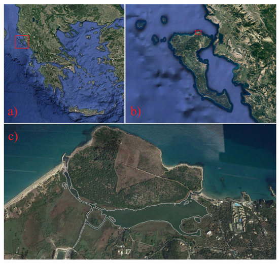
Figure 1.
(a) The location of Corfu Island on the map of Greece is shown in a red rectangle. (b) The location of Antinioti lagoon on the map of Corfu Island is shown in a red rectangle. (c) The coastline of the lagoon is marked with white color. Images from: Google Maps, 2017 [Accessed 12 August 2022].
2.2. Purpose
The purpose of the proposed methodology is the indirect estimation of the total population of the Callinectes sapidus species (blue crab) in confined environments by combining computational modeling with field measurements. The methodology is tested in Antinioti lagoon, Western Greece. More specifically, the present study addresses the question: What is the total population of blue crabs in Antinioti lagoon? This will allow for the creation of a new tool for estimating species abundance in environments where traditional methods fail in terms of precision and accuracy.
2.3. Entities, State Variables, and Scales
The proposed methodology is a combination of field measurements and simulation modeling. Therefore, the authors divide the methodology’s entities into two subcategories, the field measurements and the simulation model.
2.3.1. Field Measurements
The field measurement entities are the crab cages and time. In collaboration with local fishermen who exploit the lagoon, 25 crab cages were laid in different locations on the main body of the lagoon (the area expanding from the north to the south coast and from station 3 to station 24). The cages are coated with Polyvinyl Chloride (PVC) wire that does not rust covering an iron frame, and the net’s mesh size is 1 cm and the volume is 0.07 m3. Two oval holes exist in the middle of each side with dimensions of approximately 15 cm wide and 10 cm high. In the middle of each cage, a chicken leg was placed as bait. The cages were dropped and left in the lagoon for 24 h and then they were picked up, emptied, and counted. We selected to sample 5 times (5 days) in mid-June during the high activity of blue crabs in Antinioti lagoon. However, the fishermen use crab cages over the whole year and we have used insights from their catch to detect activity periods and chose these days as the most active within the year in Antinioti lagoon.
2.3.2. Simulation Model
The simulation model’s entities are the model’s grid, average blue crab length, average blue crab movement, time step, and simulation time. The model’s grid was created assuming that the main body of the lagoon (area between stations 1-5-11-24 Figure 2) will contain the greatest number of crab individuals (which was discussed by the fishermen and later verified by the net tows). The model’s grid has a horizontal resolution of 1000 m and a vertical resolution of 150 m. This configuration was based on the approximate distance between the north–south and east–west shores on the main body of the lagoon. However, to account for the average crab length (0.2 m from field measurements), the grid was divided by 0.2 to create a grid where each cell has the dimensions to contain one individual. Therefore, the grid’s dimensions are 5000 × 750. The time of the simulation is 24 h (as long as the cages were laid in the lagoon) divided into time steps of 100 s. All the model’s entities are static.
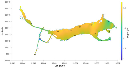
Figure 2.
The bathymetry of Antinioti lagoon and the location of the sampling stations.
2.4. Process Overview and Scheduling
This methodology’s processes involve field measurements and simulation modeling separately. The simulation model is developed to reproduce the blue crabs’ mobility in the Antinioti lagoon as it was occurring while the cages were laid in the lagoon. The simulation model’s processes are processed in the given order (Figure 3 and Figure 4).

Figure 3.
Flow chart of the methodology for blue crab population estimation.
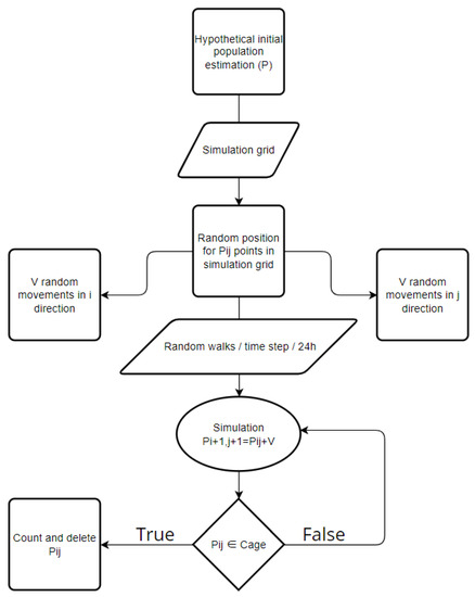
Figure 4.
Flow chart of the simulation model’s processes.
Following the random walk theory, hypothetical initial population densities with randomly placed cells start creating a stochastic path by successfully completing random steps in finite time in the selected grid (Figure 5). Each cell (representing one blue crab individual in Antinioti lagoon) will travel a random (in both length and direction) distance (per time step of 100 s) averaging 12 m/h according to the referenced mobility rate for blue crabs [86]. Each cell’s path cannot exceed the dimensions provided, keeping all crabs moving around randomly within the lagoon. The simulated movement in this confined domain is bounded by physical barriers (coastline) that act as reflecting barriers, forcing individuals to turn around and move in the opposite direction. Each path that crosses one of the 25 selected areas with dimensions 1 × 1 m (5 × 5 grid cells) is recorded and each time that these locations are crossed, it corresponds to one crab caught in the cage. The simulation ran for 24 h as long as the cages were laid in the lagoon. Each cell that is captured inside the area of a hypothetical cage is deleted from the dataset to avoid recapturing it. Each simulation ran 1000 times to estimate the mean capturing performance of the cages for the time selected.
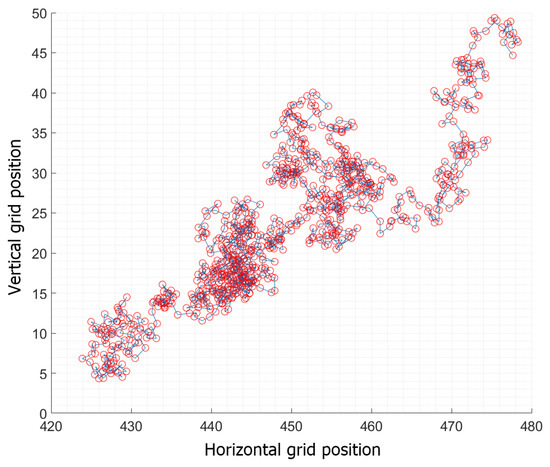
Figure 5.
An individual’s path within one iteration of 24 h for time steps of 100 s.
The methodology’s total process is the following. Firstly, a hypothetical initial population estimate is inserted in the simulation model as explained above. The second and third step is performing the simulation and determining the simulation’s outcome. The outcome of the simulation is the average population value per cage for the time of the simulation. The fourth step of the methodology is a comparison between the simulation’s result with the average population value per cage as estimated from the field measurements. Matching the simulation’s result to the number of individuals caught in real cages in the field will render us able to estimate the total blue crab population in the lagoon at the present time. If the compared values do not match, a fifth step involves multiple trials by changing the hypothetical initial population estimate and running steps 1–4 again until a match succeeds (Figure 3).
Governing Equations of Simulation Model
The mathematical code for the simulation model was created in Matlab R2021a (The Mathworks Inc., Natick, MA, USA) and included the following governing equations:
where P is the position of each individual and denote the axis direction.
where V is a stochastic spatial movement in the direction, is the average movement of individuals, and is the time step of each iteration.
2.5. Design Concepts
2.5.1. Basic Principles
The proposed methodology addresses a classic issue in ecological dynamics known as the estimation of animal density. The literature concerning this issue is extensive with several different methods applied in different species around the globe, being subject to several limitations and disadvantages, as explained in the introduction section. The present work differs from traditional methods for animal density estimation, as it combines mathematical modeling with field measurements to estimate the population abundance and then validates the results using an alternative approach based on the species’ juveniles.
2.5.2. Emergence
The methodology’s result emerges from the comparison of the simulation model and the field measurements’ average population per cage. The field measurements’ results emerge from the distribution of blue crabs in Antinioti lagoon and their attraction to bait while near a cage. The simulation model’s results emerge from the detection of virtual cages in the stochastic paths of cells representing individual blue crabs in a defined grid.
2.5.3. Adaptation
The only adaptive behavior concerning the proposed methodology is the movement of individuals, which is subject to certain limitations. Depending on the species and environment, movements can be influenced by “signals” such as chemical substances, light, temperature, and odor, among others [81,87]. These signals can attract or repel individuals and add a directional bias to their movement. Moreover, the environment may also play a role in how individuals will respond to such signals by possibly creating concentration gradients in their behavior, considering that most environments exhibit complicated barriers and terrain that will affect animal behavior and speed [81,88]. However, the above scenarios can be predicted and the possible bias can be investigated and taken into account, if there is a basic knowledge of the scattering of individuals on different time steps. In order to investigate the scattering of individuals and their abundance, and account for the above scenarios, field measurements provided data on the number of individuals sampled per sampling effort. The differences in the daily catch per cage were +/− 1 individuals, without noticing any significant differences between cages of the same sampling day, which proves that the population is well established, scattered, and sampled. Furthermore, the methodology uses a random walk algorithm to simulate the movement of individuals in the defined area. Although this simulation model could be subject to several environmental and behavioral factors (bottom habitat, depth inclinations, predation, etc) influencing the results, similar to the above assumption, the cage’s daily catch differences prove that the simulation’s results are not significantly biased by any of these factors. This is because individuals are equally sampled by all cages without showing a preference for a specific region of the sampled area.
2.6. Prediction
In the simulation model, the criteria for counting and deleting from the simulation each cell that reaches the area of a cage is based on the implicit prediction that, in reality, blue crabs that reach a cage will keep moving on its frame until they find an access point to reach the bait and therefore will definitely be trapped.
2.6.1. Sensing
Individual blue crabs are assumed to be able to sense the presence of food inside the cages when they reach the cage’s frame.
2.6.2. Interaction
The model includes no interaction among individual blue crabs.
2.6.3. Stochasticity
Stochasticity is used in the initialization of the simulation model where a hypothetical initial number of individuals are randomly placed within the grid’s area. This stochastic process allows for variability in the density of individual blue crabs at the entire extent of the grid. The stochasticity element is also being implemented in the movement of individuals, where both the speed and direction for each step are randomly selected from a database of possible spatial movements. This process is also stochastic in order to avoid unnecessary complexity in each individual’s movement.
2.6.4. Collectives
The model did not include any collectives.
2.6.5. Observation
The proposed methodology’s purpose was to estimate the total population of blue crabs in Antinioti lagoon by combining field measurements with simulation modeling. The key output observed from the field measurements was the average individual count per cage. The result observed from the simulation model was the average individual count per cage that was generated for each hypothetical initial population estimate.
2.7. Initialization
The initialization of the proposed methodology is applied to the species Callinectes sapidus of Antinioti lagoon, but can be easily applied to other species as well. However, this will require modifications regarding the field measurements and the simulation model’s parameters, depending on the species and the study area’s properties.
Simulation Model
At initialization, the state of the model at t = 0 is an environment consisting of a grid where each cell has the dimensions of the average individual’s length and therefore can contain only one individual and a hypothetical number of individuals randomly placed in cells within the grid. A data set of random movements in the i,j direction is also created based on the referenced mobility rate of individuals. Within the grid, a number of selected areas matching the number of cages that were used in the field measurements are created, with dimensions based on the actual dimensions of the real cages.
2.8. Input Data
The model does not use input data to represent time-varying processes involving environmental parameters and physical forcing.
2.9. Validation Method
Field Measurements—Juveniles
Monthly plankton net tows occurred in the lagoon from June 2020 to June 2021 (day tows). Night tows occurred in September, December, March 2020, and June 2021 covering all areas of the lagoon. Day sampling occurred at stations 1 and 12 (vertical tows) and at a range between stations 4–5, 6–8, 16–18, 20–22 (horizontal tows), shown in Figure 1, while night sampling occurred at the same stations with the addition of a vertical tow at station 16 and two horizontal tows between stations 9–12 and 24–27. The samples were collected with a plankton net with a mesh size of 53 µm having a diameter of 15 cm opening and 1 m in length. The collected samples were immobilized and preserved with 4% buffered formaldehyde solution filling 10% of the bottle for each sample to facilitate the counting process. Organisms were then counted and identified within counting chambers under a Leica S6E Stereo Microscope. Species identification was made with reference to a key determination of zooplankton species.
The filtered volume for each tow was obtained by calculating
where is the sample volume, r the net opening radius distance, and h the tow distance.
2.10. Assumptions/Limitations
The proposed methodology is a combination of field measurements and simulation processes that are subjected to a couple of assumptions/limitations. The methodology does not take into account possible cannibalistic effects in the blue crab population and inside the cages (we have found no signs to suggest that cannibalism has occurred inside the cages). Additionally, there are the factors of the cage saturation, i.e., the possibility of a crab cage being filled with crabs and not being able to sustain more inputs; the fact that bigger cages could sustain greater numbers of individuals (nevertheless, the cage’s size is one of the model’s parameters); and the possibility of other marine organisms feeding on the bait (e.g., fish). Moreover, the initial population of blue crabs in the simulation experiments is considered to be equally distributed across the lagoon’s studied area, blue crabs are expected to move constantly, and the simulated individuals are expected to be 100% captured when they encounter one of the cages.
3. Results
3.1. Field Measurements—Cages
The fishermen’s cage catch showed a differentiation during the May–October period, with a high number of individuals showing high activity in terms of crab mobility and the October–May period with at least one order of magnitude fewer individuals captured in the cages. During the first period (and our sampling dates), 13 individuals was the average daily catch per cage in Antinioti lagoon, with actual counts ranging between 12 and 14 individuals per cage, while in the months of the second period, this catch was set to fewer than 1 individual per cage per day.
Simulation Model
The model runs for 1000 iterations starting with different initial populations (N) (Figure 6 and Figure 7). As the initial population is augmented, so is the average individuals/cage/24 h, as seen in Figure 8. The average captured individuals per cage that matched the field measurements result (13 ind/cage/24 h) were reached for an initial population of 73,000 individuals, with the standard deviation being 0.71 and 949/1000 iterations being between the +/− 1 individual/cage (Figure 7).
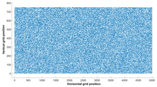
Figure 6.
Randomly placed 73,000 individual cells in the selected grid (750 × 5000) at time = 0. The grid represents Antinioti lagoon’s main area between stations 1, 5, 11, 24.
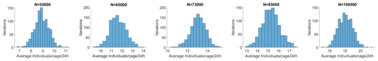
Figure 7.
Simulation model’s results after 1000 iterations for different hypothesized initial populations.
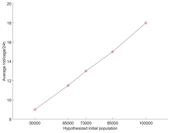
Figure 8.
Correlation curvature of simulation model’s results after 1000 iterations for different hypothesized initial populations.
3.2. Juveniles Samples
Identification of zooplankton species from the net tows under the microscope revealed the presence of blue crab juveniles in June 2020 (day) and June 2021 (day and night) but not during the rest of the year. The number of individuals was small during the day sampling with estimates of 3 ind/m3 both in June 2020 and June 2021 day, but a significant rise is observed during the June 2021 night sampling. The resulting abundance is 51 Ind/m3 for the main body of the lagoon, with more than 95% of the captured juveniles accounted for in this area.
3.3. Sensitivity
In order to test the simulation model’s sensitivity to the hypothesized initial population and the average number of individuals per cage per 24 h, we estimated the sample variance of the model’s results for the different initial populations using the following equation:
where is the sample variance, are the individual data values, is the average of the individual data values, and n is the total number of data values. The variance depends on the and , and as expected, it tends to grow, with a linear relation to the value of the average, apart from the interval (65,000, 73,000) where the variance remains constant (Figure 8 and Figure 9). As seen in Figure 7, covers similar values between 65,000 and 73,000, and as a result of that, the variance also remains similar within these two initial populations (Figure 9). Hence, the model tends to have a greater error margin as the hypothesized initial population grows. The correlation between the variance and is statistically significant with r = 0.98 and p = 0.0015 (Pearson correlation).
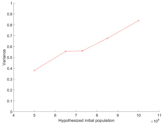
Figure 9.
Variance of simulation model’s results for different hypothesized initial populations.
4. Discussion
The initial population density of a species is the most important parameter when studying its evolution, threats, exploitation, and effect on the environment. Hence, the first step for any study of a species should be the estimation of its initial population. Here, the authors examine an innovative methodology for estimating the population abundance of the invasive species Callinectes sapidus in a confined environment. The methodology combines field measurements and the application of a simulation model based on a random walk process. Hypothesizing various potential initial populations, the authors were able to estimate the initial population producing similar results in the simulation model to the results from the field measurements.
4.1. Applicability of Proposed Methodology in Confined Environments
The proposed methodology is capable of estimating the population abundance of the invasive species in confined environments (such as Antinioti lagoon) for the following reasons. Firstly, in confined environments, individuals are forced to mobilize in a defined area surrounded by natural barriers, and therefore, the crab cages’ catch will be representative of the total population of individuals. This correlation between crab cages’ catch and the total population is one of the most significant legitimacies of such an application. In the case of an open environment, the cages’ catch could include individuals that just pass from that region and do not reside there, leading to great uncertainties in the model’s results. Secondly, the validation of the model’s result is based on the abundance of juveniles representing the adult population. Again, in the case of an open environment, sampling of blue crab juveniles would be subject to several variables (such as sea currents, predation, climate conditions, wave activity, habitat selection, depth variations, etc.) influencing the juvenile abundance. Instead, in a confined environment, the juvenile’s abundance can represent the adult population with higher precision. Lastly, the proposed approach utilizes a random walk algorithm to simulate the movement of individual blue crabs in Antinioti lagoon. Applying this algorithm requires a number of biological parameters (found in the literature) and a great understanding of the applied area’s characteristics. The advantages of confined environments in the application of the random walk algorithm are the enclosed character (natural barriers), the similar bottom habitat (sand and seagrass in the case of Antinioti lagoon), and the small depth variations (0.5–1 m in the case of Antinioti lagoon) without significant inclinations in the bottom.
4.2. Blue Crab Activity Periods in Antinioti lagoon
Due to the high numbers of blue crabs caught in the crab cages and the juvenile abundance, the species is considered to be well established in Antinioti lagoon [89]. Blue crabs experience two different phases, in terms of activity, in Antinioti lagoon. The cages’ results indicate that there are two periods with great differences in the average catch of each cage. The May–October period is considered the high-activity period where individuals move more frequently and the October–May is the inactive period where individuals tend to move as little as possible. The difference between the two periods is linked to the temperature and salinity decrease that naturally occurs during the autumn and winter months [90,91,92]. Due to its shallowness, the lagoon is directly affected by atmospheric forcing [84], and climate conditions seem to be responsible for these two activity phases.
4.3. Factors Influencing the Validation Method
Each female blue crab can produce approximately 9 million eggs annually [86]. Due to predators, fungus infections, temperature, and salinity variations, only 1 individual per million eggs will survive to become an adult [93,94]. Thus, we assume that every nine juveniles sampled in the lagoon correspond to one mature blue crab in the current population.
Diel vertical migration of zooplankton is the phenomenon where zooplankton organisms migrate from the deep water (in the sea) and from the bottom of shallow environments (Antinioti lagoon) to the surface to feed on plankton when most predators are absent [95]. At night, juvenile blue crabs, which are part of the lagoon’s zooplankton, will migrate to the surface which is the reason for the big difference between the June 2021 day and night samplings.
In order to make a rough estimate of the total population of blue crabs in Antinioti lagoon, we use the data from the night sampling since they provide a more realistic view of the actual total number of juveniles. The main body of the lagoon has the dimensions used for the model’s grid. The sampling depth is the diameter of the plankton net, which is 0.1 m. Therefore, the total number of juveniles in the main body of the lagoon is integrated from the catch of the net tows and the authors find it to be 765,000 individuals. However, every 9 of these individuals correspond to 1 female adult, so we divide the total number of juvenile individuals by 9 and get an estimate of the lagoon’s mature blue crabs of approximately 85,000.
While the values between the result of the simulation model and the juveniles’ study do not match exactly, the comparison shows that both results are in the same order of magnitude with the juveniles’ study showing a slightly greater value (≈16%). This difference may be due to the presence of blue crab populations outside Antinioti lagoon. While the lagoon’s connection to the sea is closed with a fence to prevent population exchanges for larger than 0.1 cm individuals (fish, crab, etc), young juveniles with sizes of only a few μm may enter the lagoon. Therefore, since lagoons are among the finest environments for juveniles to inhabit (protection from predators, food availability, etc.) [96], the authors believe that juveniles from blue crab populations outside the lagoon have entered and positively biased the juvenile study result.
4.4. Limitations of the Juvenile Approach
An assumption regarding the validation method and the juvenile approach is being made. The assumption is that the sampled juvenile individuals are representative of the total population of blue crabs. This assumption is being met considering that the blue crab population is bounded within Antinioti lagoon due to local fishermen’s activities and therefore cannot spawn in a different region. Additionally, juvenile samples showed that blue crab spawn occurs only once yearly, so it is not possible to overestimate the juvenile abundance by mixing individuals from different spawns.
Considering that juvenile blue crab abundances have been used to validate the simulation model’s results, several factors that may be influencing blue crab juveniles until they reach maturity are discussed. Juvenile blue crabs that grow in a coastal estuary undergo a period of 1–2 years until they become adults [97]. Therefore, there is no possibility of having measured an individual blue crab in both the juvenile and crab-trap field measurements over the course of this study.
Blue crab juveniles use several types of bottom habitats as nursery areas to stay and grow until they reach maturity [70]. These areas provide protection from predators (such as adult blue crabs [98,99,100,101]) and abundant food resources [102,103,104,105]. The sediment type of the bottom habitat does not affect the juveniles’ survival [91], while the shallowness of the environment can enhance their survival rates [106,107]. Fungus infections (Lagenidinium callinectes) and worms have been proven to be hazardous for the survival of blue crab eggs and juveniles [108,109]. However, fungi and worms only tolerate low salinity, and due to the generally high salinity encountered in Antinioti lagoon throughout most of the year, the authors do not consider these threats an issue for this study. Bauer and Miller [91] tested the effect of low temperatures and salinity on the survival rates of juvenile blue crabs over the period of 4 months. Their results showed that the survival rates drop significantly only if a combination of temperatures lower than 5 °C and salinity of 10 P.S.U. are met. In the case of Antinioti lagoon, field measurements of temperature and salinity over the course of a year showed that temperature varies between 9 and 29 °C and salinity varies between 10 and 32 P.S.U. with the lowest values lasting less than a period of 2 months. Therefore, temperature and salinity cannot significantly affect the mortality rates of juvenile blue crabs.
4.5. Implications of Proposed Methodology
The proposed methodology was proven capable of a robust prediction of the blue crab population density in Antinioti lagoon. The estimation of the current population of blue crabs is the first step for modelling the species’ evolution, which will follow in the near future. Applying this methodology to blue crab populations in confined environments will render the local authorities and fishermen that exploit the study area capable of managing their populations. This could lead to actions to preserve the population and maintain a sustainable blue crab fishery or even initiate actions for the elimination of the invasive species where it is negatively affecting the environment. This is highly important since monitoring the blue crab population using a time-efficient and low-cost approach can render the authorities able to respond quickly to potential population explosions, effectively monitoring the invasive species population and determining the effects of climate change on this ecosystem (blue crabs can act as indicators of environmental change), and they can use this methodology as a decision-making tool for managing and protecting the biodiversity of the local ecosystem. Moreover, the fishermen may want to preserve the invasive species in order to economically exploit it as a seafood product. This can lead to potential hazards for the local environment as without proper monitoring of its populations a population outburst could lead to negative effects for the lagoon’s rich biodiversity and potential conflicts with environmental organizations and the local authorities. Nevertheless, the authors believe that the novel methodology presented here exhibits benefits that could easily lead it to be adopted by the local fishermen, such as the small costs, the fast results, and the easy applicability. Additionally, the methodology is not limited to blue crabs. Following certain changes regarding the biological characteristics of the species under study and its habitat, the methodology could be applied to other invasive, endangered or common endemic species according to the need for research. In terms of the methodology’s limitations, the most significant ones are the cage saturation, the equal distribution of individual blue crabs at the initialization of the simulation experiments, the assumption of the constant movement of blue crabs, and the 100% expectation that blue crabs that encounter a cage will be captured. Considering the cage saturation, the fishermen never had issues with the selected cage sizes, and in our field measurements, the cages were never full in order to suggest that no more individuals could be captured and the results are probably biased. However, in areas with greater numbers of individuals, the possibility of cage saturation should be examined. The equal distribution of individuals was selected after getting the cages’ results (cages exhibited equal average trappabilities) and considering the fact that the bottom and depth of the lagoon are similar in the whole extent of the simulated region (Figure 2). Nevertheless, we expect that this factor may vary in other study sites and the location of cages and the distribution of individuals in the simulation’s setup should occur under careful consideration and sampling tests. The constant movement of blue crabs was decided as one of the stochastic parameters in our model (random selection of distance covered). Nevertheless, it is not always true as individual blue crabs choose randomly one value for their movement which can also be zero. Additionally, this is the peak of the active period for blue crabs and we expect to exhibit high mobility. Lastly, we decided that during the simulation, individuals that reach the area of a crab cage will be considered captured. This is because blue crabs rely on chemoreceptors to smell their food and find their way toward it [110]. Hence, in Antinioti, due to the small distance between the cage’s periphery and the bait (≤0.5 m), we expect that the species’ individuals have smelled the bait and try to find a way closer to it, which eventually leads to getting captured. However, the feeding behavior of crustaceans can be affected by several factors which should be discussed. Lobster species are commonly known to rely on their chemoreceptors to search for food. Studies have shown that once the location/direction of a potential food source is discovered, lobsters will immediately be oriented toward it [111]. Nonetheless, their feeding performance (e.g., movement speed, managing the prey, etc.) can be decreased by the potential deafferentation of their sensors and the turbulence of the water [112,113]. Moreover, studies on the green crab (Carcinus maenas) have shown that there is a significant seasonality effect affecting the appetite and feeding responses of male and female crabs, especially during the reproductive season in order to reduce the cannibalistic tendency of the species [114,115]. Additionally, climatic changes in the environmental conditions (such as global warming, CO2 concentrations, turbidity, acidification, etc.) have been shown to influence the foraging and feeding behavior of various crab species [116,117]. In terms of blue crabs, the species are known to quickly run toward the discovered odor plume and when the concentration of the odor exceeds a specific threshold at the chemoreceptors, they tend to move toward the direction of the flow [118,119]. Blue crabs usually reject prey that uses ink for protection but manipulate it longer than normal even when they sense the ink in it [120] and are also known to try to remove deterrent chemicals from food by peeling away the surface layers [121]. Blue crabs reduce foraging activity in the presence of odors that indicate the presence of predators, as shown in field [122] and laboratory experiments [123]. Nevertheless, studies have shown that even when blue crabs end up rejecting a food source, they will spend a lot of time manipulating the piece of food and will definitely find a way close to it and bite it [119,120]. Although the authors feel confident about the assumption that blue crabs that reach the area of the cage will be captured, future research is required to evaluate the aforementioned parameters and determine their effect on the cage’s trappability. Furthermore, research on the factors affecting the simulation model’s curvature (space, food availability, hydrological properties, etc.) and animal interactions is considered essential to the authors to understand the species population saturation factor and apply this curvature (Figure 8) to other marine environments.
4.6. Adaptation to Large-Scale Areas
In addition, the proposed methodology can be used to predict the population of the species in areas of greater scale than the one the present study was implemented in. In order for that to be possible: (1). One would have to: partition the larger space into smaller connected or disconnected segments. (2). Each smaller segment must be broken into its own grid, considering any possible physical barriers present in each segment. (3). Each segment must have similar conditions in the entirety of its area which would allow the researcher to use different parameters in the random walks, corresponding to the unique conditions of each segment. (4). There must be data available for the initial population estimate for each one of the segments (e.g., field sampling). (5). Each segment must be occupied by the same subspecies. (6). Possible population movement between segments must be considered. Finally, the subspecies population of all the segments can be added and a general or local population density can be estimated by taking into account the results of the model for each segment. Additionally, in order to correctly apply the methodology to estimate the population of different subspecies, a different model must be made for each subspecies and a different segmentation so that unique parameters can be defined for each run of the model (e.g., biological characteristics of the subspecies); otherwise, the results will not be correct.
4.7. Future Research
The main finding of the methodology presented here is the robust prediction of the population of an invasive species (blue crab) using a low-cost, time-effective, and easily applicable novel approach that combines field measurements and numerical simulations. Given the economic importance of the blue crab species that thrives in Antinioti lagoon, but also the potential hazards for the marine coastal ecosystems that blue crabs settle in, it is highly significant to monitor the blue crab population and manage the fishery sustainability. This can occur by assessing the stock status annually and by setting fishing policies. However, although well established, this species is known to effectively harm other valuable seafood products (fish, mollusks, etc.) in the regions it colonizes. Therefore, we need an effective evaluation of the species density fluctuations in the future, based on data available at the present time, in order to determine a decision-making tool that will render the local authorities able to protect and exploit the ecosystem by taking proper actions.
Furthermore, the continuous exploitation of the blue crabs’ stocks can facilitate population explosions as the removal of adult individuals reduces the cannibalistic effect among blue crabs and decreases the effectivity of one of the most important predators for blue crab juveniles [124]. Additionally, this may have an important effect on the social hierarchy, feeding response, and maturing behavior of juvenile crabs, as seen in other crustaceans [125]. Although this study only took place over the course of a year and exhibited no significant changes in the juveniles’ abundance, the monitoring of adult and juveniles population evolution for the next years is critical to assess the effect of the exploitation of blue crabs and the potential effect on the model’s parameters.
Additionally, previous studies in Antinioti lagoon and the NE Ionian Sea have shown that microplastic pollution is a very significant threat to the marine biodiversity of these coastal areas [126,127,128]. Due to the high abundance of marine microplastic particles in Antinioti lagoon and the economic exploitation of the blue crab species, we need to evaluate the potential ingestion of particles through the consumption of food within the lagoon by juvenile blue crabs and the potential health risks for the local population that has included the invasive species in the local cuisine.
Author Contributions
N.S.: Conceptualization, Methodology, Software, Resources, Investigation, Data curation, Writing—original draft preparation, Visualization; I.G.V.: Data curation; M.A.: Supervision, Methodology, Writing—reviewing and editing. All authors have read and agreed to the published version of the manuscript.
Funding
This research was supported by the European Union, Greece, and Italy (Cooperation Programme Interreg V-A Greece-Italy 2014–2020) under the B.E.S.T. project, which is co-funded by the European Union, European Regional Development Funds (E.R.D.F.) and by National Funds of Greece and Italy.
Institutional Review Board Statement
Not applicable.
Informed Consent Statement
Not applicable.
Data Availability Statement
Data are strictly used within the project but could be available upon request.
Acknowledgments
We wish to express our deepest gratitude and appreciation to Mike Rondos, Neophytos Sirgiotis and Mary Tzafesta for their assistance with the fieldwork. Lab work took place with the enthusiastic support of the staff of the Department of Biochemistry of the General Hospital of Corfu. More specifically, we would like to gratefully acknowledge the valuable assistance of Lilian Miari, Soula Filippa, and Anna Cheimariou.
Conflicts of Interest
The authors declare no conflict of interest.
References
- Eberhardt, L. Appraising variability in population studies. J. Wildl. Manag. 1978, 42, 207–238. [Google Scholar] [CrossRef]
- Downing, R.L.; Moore, W.H.; Kight, J. Comparison of deer census techniques applied to a known population in a Georgia enclosure. Proc. Annu. Conf. Southeast. Assoc. Game Fish Comm. 1965, 19, 26–30. [Google Scholar]
- Schmidt, J.L. A comparison of census techniques of common duiker and bushbuck in timber plantations. S. Afr. For. J. 1983, 126, 15–19. [Google Scholar] [CrossRef]
- Koster, S.H.; Hart, J.A. Methods of estimating ungulate populations in tropical forests. Afr. J. Ecol. 1988, 26, 117–126. [Google Scholar] [CrossRef]
- Mayle, B.A.; Peace, A.J.; Gill, R. How Many Deer? Forestry Commission: Edinburgh, UK, 1999. [Google Scholar]
- Hirst, S. Road-strip census techniques for wild ungulates in African woodland. J. Wildl. Manag. 1969, 33, 40–48. [Google Scholar] [CrossRef]
- Dinerstein, E. An ecological survey of the Royal Karnali-Bardia Wildlife Reserve, Nepal: Part III: Ungulate populations. Biol. Conserv. 1980, 18, 5–37. [Google Scholar] [CrossRef]
- Underwood, R. On surveying ungulate groups. Afr. J. Ecol. 1982, 20, 105–111. [Google Scholar] [CrossRef]
- Peel, M.; Bothma, J.D.P. Comparison of the accuracy of four methods commonly used to count impala. S. Afr. J. Wildl. Res. 1995, 25, 41–43. [Google Scholar]
- Reilly, B. Precision of helicopter-based total-area counts of large ungulates in bushveld. Koedoe 2002, 45, 77–83. [Google Scholar] [CrossRef]
- Bothma, J.P.; Peel, M.; Pettit, S.; Grossman, D. Evaluating the accuracy of some commonly used game-counting methods. S. Afr. J. Wildl. Res./S.-Afr. Tydskr. Natuurnavors. 1990, 20, 26–32. [Google Scholar]
- Bowland, A. Density estimate methods for blue duikers Philantomba monticola and red duikers Cephalophus natalensis in Natal, South Africa. J. Afr. Zool. 1994, 108, 505–519. [Google Scholar]
- Mandujano, S.; Gallina, S. Comparison of deer censusing methods in tropical dry forest. Wildl. Soc. Bull. 1995, 23, 180–186. [Google Scholar]
- Focardi, S.; Isotti, R.; Tinelli, A. Line transect estimates of ungulate populations in a Mediterranean forest. J. Wildl. Manag. 2002, 66, 48–58. [Google Scholar] [CrossRef]
- Lannoy, L.; Gaidet, N.; Chardonnet, P.; Fanguinoveny, M. Abundance estimates of duikers through direct counts in a rain forest, Gabon. Afr. J. Ecol. 2003, 41, 108–110. [Google Scholar] [CrossRef]
- Marsh, H.; Sinclair, D.F. Correcting for visibility bias in strip transect aerial surveys of aquatic fauna. J. Wildl. Manag. 1989, 53, 1017–1024. [Google Scholar] [CrossRef]
- Ellis, A.M. An Assessment of Density Estimation Methods for Forest Ungulates. Ph.D. Thesis, Rhodes University, Makhanda, South Africa, 2003. [Google Scholar]
- Stenson, G.; Myers, R. Accuracy of pup classifications and its effect on population estimates in the hooded seal (Cystophora cristata). Can. J. Fish. Aquat. Sci. 1988, 45, 715–719. [Google Scholar] [CrossRef]
- Bowen, W.; Myers, R.; Hay, K. Abundance estimation of a dispersed, dynamic population: Hooded seals (Cystophora cristata) in the Northwest Atlantic. Can. J. Fish. Aquat. Sci. 1987, 44, 282–295. [Google Scholar] [CrossRef]
- Burnham, K.P.; Anderson, D.R.; Laake, J.L. Estimation of density from line transect sampling of biological populations. Wildl. Monogr. 1980, 72, 3–202. [Google Scholar]
- Burnham, K.P.; Anderson, D.R. The need for distance data in transect counts. J. Wildl. Manag. 1984, 48, 1248–1254. [Google Scholar] [CrossRef]
- Bailey, R.; Putman, R. Estimation of fallow deer (Dama dama) populations from faecal accumulation. J. Appl. Ecol. 1981, 18, 697–702. [Google Scholar] [CrossRef]
- Mulligan, T.; Kieser, R. Comparison of acoustic population estimates of salmon in a lake with a weir count. Can. J. Fish. Aquat. Sci. 1986, 43, 1373–1385. [Google Scholar] [CrossRef]
- Kieser, R.; Mulligan, T.; Williamson, N.; Nelson, M. Intercalibration of two echo integration systems based on acoustic backscattering measurements. Can. J. Fish. Aquat. Sci. 1987, 44, 562–572. [Google Scholar] [CrossRef]
- Rudstam, L.G.; Clay, C.S.; Magnuson, J.J. Density and size estimates of cisco (Coregonus artedii) using analysis of echo peak PDF from a single-transducer sonar. Can. J. Fish. Aquat. Sci. 1987, 44, 811–821. [Google Scholar] [CrossRef]
- Do, M. Minimising errors in estimating fish population and biomass densities using the ‘acoustic volume backscattering strength’method. N. Z. J. Mar. Freshw. Res. 1987, 21, 99–108. [Google Scholar] [CrossRef]
- Burczynski, J.J.; Johnson, R.L. Application of dual-beam acoustic survey techniques to limnetic populations of juvenile sockeye salmon (Oncorhynchus nerka). Can. J. Fish. Aquat. Sci. 1986, 43, 1776–1788. [Google Scholar] [CrossRef]
- Buerkle, U. Estimation of fish length from acoustic target strengths. Can. J. Fish. Aquat. Sci. 1987, 44, 1782–1785. [Google Scholar] [CrossRef]
- Thomas, G.; Jackson, D.R. Acoustic measurement of fish schools using array phase information. Can. J. Fish. Aquat. Sci. 1987, 44, 1544–1550. [Google Scholar] [CrossRef]
- Nero, R.; Magnuson, J. Characterization of patches along transects using high-resolution 70-kHz integrated acoustic data. Can. J. Fish. Aquat. Sci. 1989, 46, 2056–2064. [Google Scholar] [CrossRef]
- Marques, T.A.; Thomas, L.; Martin, S.W.; Mellinger, D.K.; Ward, J.A.; Moretti, D.J.; Harris, D.; Tyack, P.L. Estimating animal population density using passive acoustics. Biol. Rev. 2013, 88, 287–309. [Google Scholar] [CrossRef]
- Seber, G.A. A review of estimating animal abundance II. Int. Stat. Rev. Int. Stat. 1992, 60, 129–166. [Google Scholar] [CrossRef]
- Keiter, D.A.; Davis, A.J.; Rhodes, O.E.; Cunningham, F.L.; Kilgo, J.C.; Pepin, K.M.; Beasley, J.C. Effects of scale of movement, detection probability, and true population density on common methods of estimating population density. Sci. Rep. 2017, 7, 9446. [Google Scholar] [CrossRef] [PubMed]
- Laplace, P.S. Sur les naissances, les mariages et les mortsa Paris depuis 1771 jusqu’a 1784 et dans toute l’étendue de la France, pendant les années 1781 et 1782. Mem. Acad. Des Sci. Present. Var. Sch. 1786, 35–46. [Google Scholar]
- Lincoln, F.C. Calculating Waterfowl Abundance on the Basis of Banding Returns; Number 118; US Department of Agriculture: Washington, DC, USA, 1930. [Google Scholar]
- White, G.C. Capture-Recapture and Removal Methods for Sampling Closed Populations; Los Alamos National Laboratory: Los Alamos, NM, USA, 1982. [Google Scholar]
- Pollock, K.H. Review papers: Modeling capture, recapture, and removal statistics for estimation of demographic parameters for fish and wildlife populations: Past, present, and future. J. Am. Stat. Assoc. 1991, 86, 225–238. [Google Scholar] [CrossRef]
- Jolly, G.M. Explicit estimates from capture-recapture data with both death and immigration-stochastic model. Biometrika 1965, 52, 225–247. [Google Scholar] [CrossRef] [PubMed]
- Seber, G.A. A note on the multiple-recapture census. Biometrika 1965, 52, 249–259. [Google Scholar] [CrossRef]
- Seber, G.A.F. The estimation of Animal Abundance and Related Parameters; Blackburn Press: Caldwell, NJ, USA, 1982. [Google Scholar]
- Parmenter, R.R.; Yates, T.L.; Anderson, D.R.; Burnham, K.P.; Dunnum, J.L.; Franklin, A.B.; Friggens, M.T.; Lubow, B.C.; Miller, M.; Olson, G.S.; et al. Small-mammal density estimation: A field comparison of grid-based vs. web-based density estimators. Ecol. Monogr. 2003, 73, 1–26. [Google Scholar] [CrossRef]
- Buckland, S. A mark-recapture survival analysis. J. Anim. Ecol. 1982, 51, 833–847. [Google Scholar] [CrossRef]
- Janečka, J.E.; Munkhtsog, B.; Jackson, R.M.; Naranbaatar, G.; Mallon, D.P.; Murphy, W.J. Comparison of noninvasive genetic and camera-trapping techniques for surveying snow leopards. J. Mammal. 2011, 92, 771–783. [Google Scholar] [CrossRef]
- Burgar, J.M.; Stewart, F.E.; Volpe, J.P.; Fisher, J.T.; Burton, A.C. Estimating density for species conservation: Comparing camera trap spatial count models to genetic spatial capture-recapture models. Glob. Ecol. Conserv. 2018, 15, e00411. [Google Scholar] [CrossRef]
- Davis, A.J.; Keiter, D.A.; Kierepka, E.M.; Slootmaker, C.; Piaggio, A.J.; Beasley, J.C.; Pepin, K.M. A comparison of cost and quality of three methods for estimating density for wild pig (Sus scrofa). Sci. Rep. 2020, 10, 2047. [Google Scholar] [CrossRef] [PubMed]
- McCallum, J. Changing use of camera traps in mammalian field research: Habitats, taxa and study types. Mammal Rev. 2013, 43, 196–206. [Google Scholar] [CrossRef]
- Royle, J.A.; Young, K.V. A hierarchical model for spatial capture—Recapture data. Ecology 2008, 89, 2281–2289. [Google Scholar] [CrossRef] [PubMed]
- Efford, M.G.; Dawson, D.K.; Borchers, D.L. Population density estimated from locations of individuals on a passive detector array. Ecology 2009, 90, 2676–2682. [Google Scholar] [CrossRef]
- Burton, A.C.; Neilson, E.; Moreira, D.; Ladle, A.; Steenweg, R.; Fisher, J.T.; Bayne, E.; Boutin, S. Wildlife camera trapping: A review and recommendations for linking surveys to ecological processes. J. Appl. Ecol. 2015, 52, 675–685. [Google Scholar] [CrossRef]
- Rowcliffe, J.M.; Field, J.; Turvey, S.T.; Carbone, C. Estimating animal density using camera traps without the need for individual recognition. J. Appl. Ecol. 2008, 45, 1228–1236. [Google Scholar] [CrossRef]
- Rowcliffe, J.M.; Kays, R.; Kranstauber, B.; Carbone, C.; Jansen, P.A. Quantifying levels of animal activity using camera trap data. Methods Ecol. Evol. 2014, 5, 1170–1179. [Google Scholar] [CrossRef]
- Anile, S.; Ragni, B.; Randi, E.; Mattucci, F.; Rovero, F. Wildcat population density on the E tna volcano, I taly: A comparison of density estimation methods. J. Zool. 2014, 293, 252–261. [Google Scholar] [CrossRef]
- Balestrieri, A.; Ruiz-González, A.; Vergara, M.; Capelli, E.; Tirozzi, P.; Alfino, S.; Minuti, G.; Prigioni, C.; Saino, N. Pine marten density in lowland riparian woods: A test of the Random Encounter Model based on genetic data. Mamm. Biol. 2016, 81, 439–446. [Google Scholar] [CrossRef]
- Caravaggi, A.; Zaccaroni, M.; Riga, F.; Schai-Braun, S.C.; Dick, J.T.; Montgomery, W.I.; Reid, N. An invasive-native mammalian species replacement process captured by camera trap survey random encounter models. Remote Sens. Ecol. Conserv. 2016, 2, 45–58. [Google Scholar] [CrossRef]
- Carbajal-Borges, J.P.; Godínez-Gómez, O.; Mendoza, E. Density, abundance and activity patterns of the endangered Tapirus bairdii in one of its last strongholds in southern Mexico. Trop. Conserv. Sci. 2014, 7, 100–114. [Google Scholar] [CrossRef]
- Manzo, E.; Bartolommei, P.; Rowcliffe, J.M.; Cozzolino, R. Estimation of population density of European pine marten in central Italy using camera trapping. Acta Theriol. 2012, 57, 165–172. [Google Scholar] [CrossRef]
- Cusack, J.J.; Swanson, A.; Coulson, T.; Packer, C.; Carbone, C.; Dickman, A.J.; Kosmala, M.; Lintott, C.; Rowcliffe, J.M. Applying a random encounter model to estimate lion density from camera traps in Serengeti National Park, Tanzania. J. Wildl. Manag. 2015, 79, 1014–1021. [Google Scholar] [CrossRef] [PubMed]
- Rademaker, M.; Meijaard, E.; Semiadi, G.; Blokland, S.; Neilson, E.W.; Rode-Margono, E.J. First ecological study of the Bawean warty pig (Sus blouchi), one of the rarest pigs on earth. PLoS ONE 2016, 11, e0151732. [Google Scholar] [CrossRef] [PubMed]
- Rovero, F.; Marshall, A.R. Camera trapping photographic rate as an index of density in forest ungulates. J. Appl. Ecol. 2009, 46, 1011–1017. [Google Scholar] [CrossRef]
- Zero, V.H.; Sundaresan, S.R.; O’Brien, T.G.; Kinnaird, M.F. Monitoring an endangered savannah ungulate, Grevy’s zebra Equus grevyi: Choosing a method for estimating population densities. Oryx 2013, 47, 410–419. [Google Scholar] [CrossRef]
- Nakashima, Y.; Fukasawa, K.; Samejima, H. Estimating animal density without individual recognition using information derivable exclusively from camera traps. J. Appl. Ecol. 2018, 55, 735–744. [Google Scholar] [CrossRef]
- Nakashima, Y. Potentiality and limitations of N-mixture and Royle-Nichols models to estimate animal abundance based on noninstantaneous point surveys. Popul. Ecol. 2020, 62, 151–157. [Google Scholar] [CrossRef]
- consortium, E.; Grignolio, S.; Apollonio, M.; Brivio, F.; Vicente, J.; Acevedo, P.; Petrovic, K.; Keuling, O. Guidance on estimation of abundance and density data of wild ruminant population: Methods, challenges, possibilities. EFSA Support. Publ. 2020, 17, 1876E. [Google Scholar]
- Schwarz, C.J.; Seber, G.A. Estimating animal abundance: Review III. Stat. Sci. 1999, 14, 427–456. [Google Scholar] [CrossRef]
- Vargas Soto, J.S.; Castañeda, R.A.; Mandrak, N.E.; Molnár, P.K. Estimating animal density in three dimensions using capture-frequency data from remote detectors. Remote Sens. Ecol. Conserv. 2021, 7, 36–49. [Google Scholar] [CrossRef]
- Bell, M.; Eaton, D.; Bannister, R.; Addison, J. A mark-recapture approach to estimating population density from continuous trapping data: Application to edible crabs, Cancer pagurus, on the east coast of England. Fish. Res. 2003, 65, 361–378. [Google Scholar] [CrossRef]
- Millikin, M.R. Synopsis of Biological Data on the Blue Crab, Callinectes sapidus Rathbun; Number 138; National Oceanic and Atmospheric Administration, National Marine Fisheries: Washington, DC, USA, 1984. [Google Scholar]
- Nehring, S. Invasion history and success of the American blue crab Callinectes sapidus in European and adjacent waters. In the Wrong Place-Alien Marine Crustaceans: Distribution, Biology and Impacts; Springer: Berlin/Heidelberg, Germany, 2011; pp. 607–624. [Google Scholar]
- Williams, A.B. The swimming crabs of the genus Callinectes (Decapoda: Portunidae). Fish. Bull. 1971, 72, 685. [Google Scholar]
- Hines, A.; Kennedy, V.; Cronin, L. The Blue Crab Callinectes sapidus; MD Sea Grant College Press: College Park, MD, USA, 2007. [Google Scholar]
- Perkins-Visser, E.; Wolcott, T.G.; Wolcott, D.L. Nursery role of seagrass beds: Enhanced growth of juvenile blue crabs (Callinectes sapidus Rathbun). J. Exp. Mar. Biol. Ecol. 1996, 198, 155–173. [Google Scholar] [CrossRef]
- Mancinelli, G.; Chainho, P.; Cilenti, L.; Falco, S.; Kapiris, K.; Katselis, G.; Ribeiro, F. The Atlantic blue crab Callinectes sapidus in southern European coastal waters: Distribution, impact and prospective invasion management strategies. Mar. Pollut. Bull. 2017, 119, 5–11. [Google Scholar] [CrossRef]
- BouvıER, E. Sur un Callinectes sapidus M. Rathbun trouvé à Rocheford. Bull. Mus. Hist. Naf, Paris 1901, 7, 66. [Google Scholar]
- Enzenro, R.; Enzenro, L.; Bİngel, F. Occurrence of blue crab, Callinectes sapidus (Rathbun, 1896) (Crustacea, Brachyura) on the Turkish Mediterranean and the adjacent Aegean coast and its size distribution in the bay of Iskenderun. Turk. J. Zool. 1997, 21, 113–122. [Google Scholar] [CrossRef]
- Labrune, C.; Amilhat, E.; Amouroux, J.M.; Coraline, J.; Alexandra, G.; Noël, P.Y. The arrival of the American blue crab, Callinectes sapidus Rathbun, 1896 (Decapoda: Brachyura: Portunidae), in the Gulf of lions (Mediterranean Sea). Bioinvasions Rec. 2019, 8, 876–881. [Google Scholar] [CrossRef]
- Massé, C.; Viard, F.; Humbert, S.; Antajan, E.; Auby, I.; Bachelet, G.; Bernard, G.; Bouchet, V.M.; Burel, T.; Dauvin, J.C.; et al. An overview of marine non-indigenous species found in three contrasting biogeographic metropolitan French regions: Insights on distribution, origins and pathways of introduction. Diversity 2023, 15, 161. [Google Scholar] [CrossRef]
- Kapiris, K.; Apostolidis, C.; Baldacconi, R.; Başusta, N.; Bilecenoglu, M.; Bitar, G.; Bobori, D.; Boyaci, Y.Ö.; Dimitriadis, C.; Djurović, M.; et al. New Mediterranean Biodiversity Records (April, 2014). Mediterr. Mar. Sci. 2014, 15, 198–212. [Google Scholar] [CrossRef]
- Bilecenoglu, M.; Alfaya, J.E.; Azzurro, E.; Baldacconi, R.; Boyaci, Y.; Circosta, V.; Compagno, L.; Coppola, F.; Deidun, A.; Durgham, H.; et al. New Mediterranean marine biodiversity records (December, 2013). Mediterr. Mar. Sci. 2013, 14, 463–480. [Google Scholar] [CrossRef]
- Perdikaris, C.; Konstantinidis, E.; Gouva, E.; Ergolavou, A.; Klaoudatos, D.; Nathanailides, C.; Paschos, I. Occurrence of the invasive crab species Callinectes sapidus Rathbun, 1896, in NW Greece. Walailak J. Sci. Technol. (WJST) 2016, 13, 503–510. [Google Scholar]
- Carrozzo, L.; Potenza, L.; Carlino, P.; Costantini, M.L.; Rossi, L.; Mancinelli, G. Seasonal abundance and trophic position of the Atlantic blue crab Callinectes sapidus Rathbun 1896 in a Mediterranean coastal habitat. Rend. Lincei 2014, 25, 201–208. [Google Scholar] [CrossRef]
- Codling, E.A.; Plank, M.J.; Benhamou, S. Random walk models in biology. J. R. Soc. Interface 2008, 5, 813–834. [Google Scholar] [CrossRef] [PubMed]
- Grimm, V.; Berger, U.; Bastiansen, F.; Eliassen, S.; Ginot, V.; Giske, J.; Goss-Custard, J.; Grand, T.; Heinz, S.K.; Huse, G.; et al. A standard protocol for describing individual-based and agent-based models. Ecol. Model. 2006, 198, 115–126. [Google Scholar] [CrossRef]
- Grimm, V.; Berger, U.; DeAngelis, D.L.; Polhill, J.G.; Giske, J.; Railsback, S.F. The ODD protocol: A review and first update. Ecol. Model. 2010, 221, 2760–2768. [Google Scholar] [CrossRef]
- Simantiris, N.; Theocharis, A.; Avlonitis, M. Environmental effects on zooplankton dynamics of a shallow Mediterranean coastal lagoon (October 2020–March 2021). Reg. Stud. Mar. Sci. 2021, 48, 102001. [Google Scholar] [CrossRef]
- Simantiris, N.; Avlonitis, M. Effects of future climate conditions on the zooplankton of a Mediterranean coastal lagoon. Estuarine, Coast. Shelf Sci. 2023, 282, 108231. [Google Scholar] [CrossRef]
- Hines, A.H.; Lipcius, R.N.; Haddon, A.M. Population dynamics and habitat partitioning by size, sex, and molt stage of blue crabs Callinectes sapidus in a subestuary of central Chesapeake Bay. Mar. Ecol. Prog. Ser. 1987, 36, 55–64. [Google Scholar] [CrossRef]
- Cai, A.Q.; Landman, K.A.; Hughes, B.D. Modelling directional guidance and motility regulation in cell migration. Bull. Math. Biol. 2006, 68, 25–52. [Google Scholar] [CrossRef]
- Vuilleumier, S.; Metzger, R. Animal dispersal modelling: Handling landscape features and related animal choices. Ecol. Model. 2006, 190, 159–170. [Google Scholar] [CrossRef]
- Kara, M.H.; Chaoui, L. Strong invasion of Mellah lagoon (South-Western Mediterranean) by the American blue crab Callinectes sapidus Rathbun, 1896. Mar. Pollut. Bull. 2021, 164, 112089. [Google Scholar] [CrossRef] [PubMed]
- Leffler, C. Some effects of temperature on the growth and metabolic rate of juvenile blue crabs, Callinectes sapidus, in the laboratory. Mar. Biol. 1972, 14, 104–110. [Google Scholar] [CrossRef]
- Bauer, L.J.; Miller, T.J. Temperature-, salinity-, and size-dependent winter mortality of juvenile blue crabs (Callinectes sapidus). Estuaries Coasts 2010, 33, 668–677. [Google Scholar] [CrossRef]
- Jakov, D.; Glamuzina, B. Six years from first record to population establishment: The case of the blue crab, Callinectes sapidus Rathbun, 1896 (Brachyura, Portunidae) in the Neretva River delta (South-eastern Adriatic Sea, Croatia). Crustaceana 2011, 84, 1211–1220. [Google Scholar]
- Couch, J.N. A new fungus on crab eggs. J. Elisha Mitchell Sci. Soc. 1942, 58, 158–162. [Google Scholar]
- Van Engel, W.A. The blue crab and its fishery in Chesapeake Bay. Part 1. Reproduction, early development, growth and migration. Commer. Fish. Rev. 1958, 20, 6. [Google Scholar]
- Lampert, W. The adaptive significance of diel vertical migration of zooplankton. Funct. Ecol. 1989, 3, 21–27. [Google Scholar] [CrossRef]
- Buchanan, B.A.; Stoner, A.W. Distributional patterns of blue crabs (Callinectes sp.) in a tropical estuarine lagoon. Estuaries 1988, 11, 231–239. [Google Scholar] [CrossRef]
- Hines, A.H.; Jivoff, P.R.; Bushmann, P.J.; van Montfrans, J.; Reed, S.A.; Wolcott, D.L.; Wolcott, T.G. Evidence for sperm limitation in the blue crab, Callinectes sapidus. Bull. Mar. Sci. 2003, 72, 287–310. [Google Scholar]
- Dittel, A.I.; Hines, A.H.; Ruiz, G.M.; Ruffin, K.K. Effects of shallow water refuge on behavior and density-dependent mortality of juvenile blue crabs in Chesapeake Bay. Bull. Mar. Sci. 1995, 57, 902–916. [Google Scholar]
- Orth, R.J.; VANMONTFRANS, J. Utilization of a seagrass meadow and tidal marsh creek by blue crabs Callinectes sapidus. I. Seasonal and annual variations in abundance with emphasis on post-settlement juveniles. Mar. Ecol. Prog. Ser. 1987, 41, 283. [Google Scholar] [CrossRef]
- Hovel, K.A.; Lipcius, R.N. Habitat fragmentation in a seagrass landscape: Patch size and complexity control blue crab survival. Ecology 2001, 82, 1814–1829. [Google Scholar] [CrossRef]
- Hovel, K.A.; Fonseca, M.S. Influence of seagrass landscape structure on the juvenile blue crab habitat-survival function. Mar. Ecol. Prog. Ser. 2005, 300, 179–191. [Google Scholar] [CrossRef]
- Beck, M.W.; Heck, K.L.; Able, K.W.; Childers, D.L.; Eggleston, D.B.; Gillanders, B.M.; Halpern, B.; Hays, C.G.; Hoshino, K.; Minello, T.J.; et al. The identification, conservation, and management of estuarine and marine nurseries for fish and invertebrates: A better understanding of the habitats that serve as nurseries for marine species and the factors that create site-specific variability in nursery quality will improve conservation and management of these areas. Bioscience 2001, 51, 633–641. [Google Scholar]
- Seitz, R.D.; Knick, K.E.; Westphal, M. Diet selectivity of juvenile blue crabs (Callinectes sapidus) in Chesapeake Bay. Integr. Comp. Biol. 2011, 51, 598–607. [Google Scholar] [CrossRef]
- Litvin, S.Y.; Weinstein, M.P.; Sheaves, M.; Nagelkerken, I. What makes nearshore habitats nurseries for nekton? An emerging view of the nursery role hypothesis. Estuaries Coasts 2018, 41, 1539–1550. [Google Scholar] [CrossRef]
- Epifanio, C.E.; Dittel, A.; Rodriguez, R.A.; Targett, T.E. The role of macroalgal beds as nursery habitat for juvenile blue crabs, Callinectes sapidus. J. Shellfish Res. 2003, 22, 881–886. [Google Scholar]
- Ruiz, G.M.; Hines, A.H.; Posey, M.H. Shallow water as a refuge habitat for fish and crustaceans in non-vegetated estuaries: An example from Chesapeake Bay. Mar. Ecol. Prog. Ser. 1993, 99, 1–16. [Google Scholar] [CrossRef]
- Hines, A.H.; Ruiz, G.M. Temporal variation in juvenile blue crab mortality: Nearshore shallows and cannibalism in Chesapeake Bay. Bull. Mar. Sci. 1995, 57, 884–901. [Google Scholar]
- Rogers-Talbert, R. The fungus Lagenidium callinectes Couch (1942) on eggs of the blue crab in Chesapeake Bay. Biol. Bull. 1948, 95, 214–228. [Google Scholar] [CrossRef] [PubMed]
- Shields, J.D. Research priorities for diseases of the blue crab Callinectes sapidus. Bull. Mar. Sci. 2003, 72, 505. [Google Scholar]
- Pearson, W.H.; Olla, B.L. Chemoreception in the blue crab, Callinectes sapidus. Biol. Bull. 1977, 153, 346–354. [Google Scholar] [CrossRef]
- Devine, D.V.; Atema, J. Function of chemoreceptor organs in spatial orientation of the lobster, Homarus americanus: Differences and overlap. Biol. Bull. 1982, 163, 144–153. [Google Scholar] [CrossRef]
- Moore, P.A.; Scholz, N.; Atema, J. Chemical orientation of lobsters, Homarus americanus, in turbulent odor plumes. J. Chem. Ecol. 1991, 17, 1293–1307. [Google Scholar] [CrossRef] [PubMed]
- Derby, C.D.; Atema, J. The function of chemo-and mechanoreceptors in lobster (Homarus americanus) feeding behaviour. J. Exp. Biol. 1982, 98, 317–327. [Google Scholar] [CrossRef]
- Hayden, D.; Jennings, A.; Müller, C.; Pascoe, D.; Bublitz, R.; Webb, H.; Breithaupt, T.; Watkins, L.; Hardege, J. Sex-specific mediation of foraging in the shore crab, Carcinus maenas. Horm. Behav. 2007, 52, 162–168. [Google Scholar] [CrossRef]
- Hardege, J.; Bartels-Hardege, H.; Fletcher, N.; Terschak, J.; Harley, M.; Smith, M.; Davidson, L.; Hayden, D.; Müller, C.T.; Lorch, M.; et al. Identification of a female sex pheromone in Carcinus maenas. Mar. Ecol. Prog. Ser. 2011, 436, 177–189. [Google Scholar] [CrossRef]
- Draper, A.M.; Weissburg, M.J. Impacts of global warming and elevated CO2 on sensory behavior in predator-prey interactions: A review and synthesis. Front. Ecol. Evol. 2019, 7, 72. [Google Scholar] [CrossRef]
- Richardson, B.; Martin, H.; Bartels-Hardege, H.; Fletcher, N.; Hardege, J.D. The role of changing pH on olfactory success of predator–prey interactions in green shore crabs, Carcinus maenas. Aquat. Ecol. 2022, 56, 409–418. [Google Scholar] [CrossRef]
- Page, J.L.; Dickman, B.D.; Webster, D.R.; Weissburg, M.J. Getting ahead: Context-dependent responses to odorant filaments drive along-stream progress during odor tracking in blue crabs. J. Exp. Biol. 2011, 214, 1498–1512. [Google Scholar] [CrossRef]
- Aggio, J.F.; Tieu, R.; Wei, A.; Derby, C.D. Oesophageal chemoreceptors of blue crabs, Callinectes sapidus, sense chemical deterrents and can block ingestion of food. J. Exp. Biol. 2012, 215, 1700–1710. [Google Scholar] [CrossRef]
- Aggio, J.F.; Derby, C.D. Hydrogen peroxide and other components in the ink of sea hares are chemical defenses against predatory spiny lobsters acting through non-antennular chemoreceptors. J. Exp. Mar. Biol. Ecol. 2008, 363, 28–34. [Google Scholar] [CrossRef]
- Kamio, M.; Grimes, T.V.; Hutchins, M.H.; van Dam, R.; Derby, C.D. The purple pigment aplysioviolin in sea hare ink deters predatory blue crabs through their chemical senses. Anim. Behav. 2010, 80, 89–100. [Google Scholar] [CrossRef]
- Ferner, M.C.; Smee, D.L.; Chang, Y.P. Cannibalistic crabs respond to the scent of injured conspecifics: Danger or dinner? Mar. Ecol. Prog. Ser. 2005, 300, 193–200. [Google Scholar] [CrossRef]
- Moir, F.; Weissburg, M. Cautious cannibals: Behavioral responses of juvenile and adult blue crabs to the odor of injured conspecifics. J. Exp. Mar. Biol. Ecol. 2009, 369, 87–92. [Google Scholar] [CrossRef]
- Grosholz, E.; Ashton, G.; Bradley, M.; Brown, C.; Ceballos-Osuna, L.; Chang, A.; de Rivera, C.; Gonzalez, J.; Heineke, M.; Marraffini, M.; et al. Stage-specific overcompensation, the hydra effect, and the failure to eradicate an invasive predator. Proc. Natl. Acad. Sci. USA 2021, 118, e2003955118. [Google Scholar] [CrossRef] [PubMed]
- Wang, C.; Li, S.; Fu, C.; Gong, X.; Huang, L.; Song, X.; Zhao, Y. Molecular genetic structure and evolution in native and colonized populations of the Chinese mitten crab, Eriocheir sinensis. Biol. Invasions 2009, 11, 389–399. [Google Scholar] [CrossRef]
- Simantiris, N.; Vardaki, M.Z.; Koralli, P.; Chochos, C.L.; Gregoriou, V.G.; Kourkoumelis, N.; Avlonitis, M. Seasonal evaluation of floating microplastics in a shallow Mediterranean coastal lagoon: Abundance, distribution, chemical composition, and influence of environmental factors. Estuarine, Coast. Shelf Sci. 2022, 272, 107859. [Google Scholar] [CrossRef]
- Simantiris, N.; Avlonitis, M.; Theocharis, A. Simulation of the transport of marine microplastic particles in the Ionian Archipelago (NE Ionian Sea) using a Lagrangian model and the control mechanisms affecting their transport. J. Hazard. Mater. 2022, 437, 129349. [Google Scholar] [CrossRef]
- Simantiris, N.; Vardaki, M.Z.; Kourkoumelis, N.; Avlonitis, M.; Theocharis, A. Microplastics in the Mediterranean and Elsewhere in Coastal Seas; Elsevier: Amsterdam, The Netherlands, 2023; in press. [Google Scholar]


Disclaimer/Publisher’s Note: The statements, opinions and data contained in all publications are solely those of the individual author(s) and contributor(s) and not of MDPI and/or the editor(s). MDPI and/or the editor(s) disclaim responsibility for any injury to people or property resulting from any ideas, methods, instructions or products referred to in the content. |
© 2023 by the authors. Licensee MDPI, Basel, Switzerland. This article is an open access article distributed under the terms and conditions of the Creative Commons Attribution (CC BY) license (https://creativecommons.org/licenses/by/4.0/).