ABiLSTM Based Prediction Model for AUV Trajectory

Abstract

On 25 July 2021, the AUV of the Marine Science and Technology Research Center was lost under the sea due to a fracture of the wire rope when it was performing a mission offshore of China. A model is presented in the paper for predicting the trajectory of a lost AUV based on ABiLSTM. To increase the precision of model prediction, the model incorporates the soft attention mechanism and is based on the bidirectional Long Short-Term Memory (BiLSTM) network. In comparison to LSTM, BiLSTM, and attention-LSTM models, experiments have demonstrated that the proposed model enhanced prediction accuracy in terms of longitude, latitude, and altitude by 0.009° E, 0.008° N, and 2 m using representative root mean squared error as an assessment indicator. The findings of the study can improve marine rescue efforts and aid in the search and recovery of AUVs that have crashed.

1. Introduction

In recent years, with China’s accelerated exploration of the ocean, autonomous underwater vehicles have realized autonomous navigation in the ocean because of their small size, lightweight, and strong flexibility. They have played a huge role in the fields of ocean exploration, undersea search and rescue, marine resource development, and so on. One of the main concerns in its study and use is the safety of AUV navigation in a complex marine environment [1]. Due to both the complexity of the underwater environment and the lack of human insight into the maritime environment, the AUV may be disconnected and lost. The safety of the AUV has been highly questioned by researchers in this field [2,3]. The prediction of the AUV’s trajectory is an effective and crucial method for searching for and rescuing the lost AUV. The sensors installed on the AUV body are used in a traditional trajectory prediction method to obtain its underwater position and related information, and then connect this information with the target state to carry out mathematical calculations to obtain the position of the aim. The position of each step toward the goal is finally used to forecast the navigation trajectory. Luo et al. discussed the prediction of the state of the target through target identification, determination of location, building of the target model, and then predicting the trajectory [4]. With the rise of neural networks, many researchers try to build neural network models to predict trajectories. Using a mathematical model called a neural network, one can process information by simulating the synaptic connection structure of the human brain, which can be used for trajectory prediction. Jiansen Zhao et al. proposed an integrated machine learning framework to process AIS data and predict ship trajectory trends [5]. Inspired by the powerful learning ability of deep neural networks, Ryan Wen Liu et al. proposed an AIS data-driven trajectory prediction framework [6]. The back-propagation neural network approach was utilized by Xu et al. and Zhou et al. to forecast ship trajectories by learning the observed data of ship navigation parameters [7,8]. A RNN, in terms of network topology, is a typical neural network that retains prior knowledge and makes use of it to affect the output of later nodes. Its main purpose is to process and predict sequence data, such as speech recognition, text translation, and language modeling. AUV trajectory data is time-series trajectory data, so an AUV trajectory can be predicted by an RNN neural network. However, when RNN trains its parameters through a back-propagation algorithm, it is very possible for gradient problems like disappearance and explosion to arise, which can be well solved by the LSTM model and the GRU model [9,10]. The LSTM neural network and the GRU neural network have successfully demonstrated good performance in sequence applications [11,12,13]. BiLSTM is made up of forward and backward LSTM. Its prediction model is more accurate than the LSTM neural network [14]. Jia and Chen et al. put forward an attention-based LSTM trajectory prediction model [15]. This model processes four-dimensional aircraft trajectory data consisting of time, longitude, latitude, and altitude, incorporates an attention mechanism to learn feature weights, predicts flight trajectories, and compares this model with the classical LSTM model and support vector machine model. The experimental outcomes demonstrate that this approach enhances trajectory prediction accuracy. Jiating Yin et al. constructed a new Long short-term memory (LAG-LSTM) model with delayed information and then constructed a data-driven train control model (TCM) to accurately predict the long-term trajectory of high-speed trains [16]. Xiping Wu et al. proposed a new long-term 4D trajectory prediction model based on a generative adversarial network (GAN) that is used to predict the historical 4D aviation trajectory from Beijing to Chengdu, China [17]. The attention mechanism is a model established by Treisman and Gelade to imitate human brain attention that is widely utilized in the subject of deep learning [18,19]. Shaojiang Dong et al. extracted global and temporal information using convolutional networks and bidirectional Long short-term memory (Bi-LSTM), and combined attention mechanisms to forecast the remaining life of rolling bearings [20]. In light of this, an ABiLSTM model for trajectory prediction of AUV is proposed, and its performance is compared with LSTM, BiLSTM, and Attention-LSTM models. The following are the primary contributions to this paper:

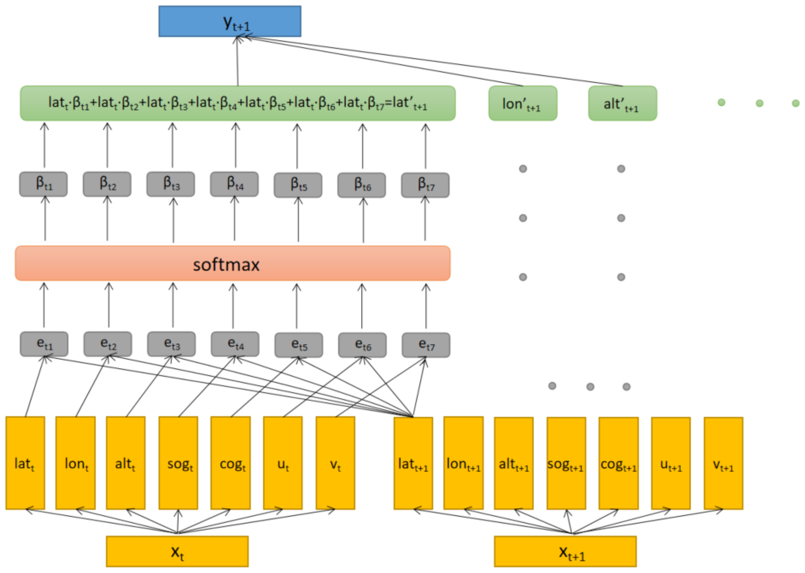
• The ABiLSTM model for AUV trajectory prediction is proposed. The trajectory prediction issue is regarded as a time series prediction problem in this work. In order to increase the accuracy of AUV trajectory prediction, the features of the data are extracted, and the attention mechanism is utilized to boost the contribution of important aspects and decrease the effect of unimportant elements.
• Different factors influencing AUV trajectory prediction are considered, such as historical AUV trajectory data and ocean current influencing factors. In this paper, historical AUV track data is a time series that considers not only the longitude, latitude, and altitude information of AUV historical data points but also the course over ground and speed over ground of AUV and ocean current information about the position of the lost AUV in the ocean to improve data variety.
• A sliding-window data training approach is used. Using the historical trajectory information in the time window to forecast the development direction of the next moment in the future can ensure the continuity of data, which is more conducive to model training and trajectory prediction.

The remaining portions of this paper are structured as follows: The second section describes the principles and structure details of several popular neural network models and the model proposed. The third part describes the contents of this experiment in detail, and the model suggested is contrasted with other commonly used models to verify the accuracy of this model in predicting AUV trajectory. Additionally, do more ship trajectory prediction tests to demonstrate the recommended model’s adaptation. The fourth part puts forward the conclusion and prospects for the work to come.

2. Model Description

In this section, several neural network models are introduced, including the recurrent neural network model, the LSTM model, the BiLSTM model, and the Attention-LSTM model. These models are described in detail below. Based on these models, an improved trajectory prediction model based on ABiLSTM is proposed.

2.1. Recurrent Neural Network Model

A RNN is a recursive neural network that is particularly useful for handling time-series tasks [21]. Natural language is usually arranged in chronological order. In the field of natural language processing, time series usually refers to a series of words or sentences in chronological order. Each of these words or sentences contains a wealth of semantic information, such as emotion, theme, mood, etc. These pieces of information are interrelated in time. Therefore, the RNN model can be used for speech recognition, text classification, machine translation, and other tasks. Because sequence data typically has a non-linear time dependency, the current output is affected by multiple previous inputs. The memory of recurrent neural networks can utilize previous information to learn this complex nonlinear relationship, making it more suitable for learning the nonlinear features of sequences. Figure 1 displays the RNN structure.

As shown in Figure 1, RNN is the most basic single-layer network, which is expanded on the time series. At time t, the input is $x_t$. After the following transformation, the hidden layer $s_t$ at time t is acquired, which is also the output $y_t$ at time t.

$$s_t=f(U{x}_t+W{s}_{t-1}+b)$$

(1)

where f stands for the activation function, U stands for the weight that is delivered from the input layer to the hidden layer, W is the self-recursive weight of the hidden layer, and b is the deviation value. U and W are the same at every moment; that is, the parameters at every moment are shared, which is also one of the important characteristics of RNN.

2.2. LSTM Model

LSTM is an RNN gating algorithm. An array of LSTM units makes up the LSTM network, each of which has three gates (an input gate, a forgetting gate, and an output gate) and one state unit. They include the state unit, which stores information about the current state; the forgetting gate, which regulates the retention of past states; the output gate, which regulates the creation of outputs; and the input gate, which regulates the influence of incoming inputs. The gate mechanism allows LSTM networks to more effectively manage information flow and storage, better capturing long-term relationships in sequences. By using LSTM, the generic RNN’s long-term reliance issue is resolved, and the RNN’s inadequacies of gradient disappearance and gradient explosion are addressed [22]. Figure 2 depicts one LSTM unit’s internal design.

In Figure 2, $\sigma$ is the sigmoid activation function. Its output is between 0 and 1, as shown below:

$$\sigma \left(x\right)=\frac{1}{1+e^{-x}}$$

(2)

$tanh$ is an activation function used to update the hidden state of LSTM. Its output is between −1 and 1, as shown below:

$$tanh\left(x\right)=\frac{1-e^{-x}}{1+e^{-x}}$$

(3)

$I_t$ represents the input at time t, and $h{d}_t$ is the hidden state at this time. Compared with the hidden layer of the original RNN, LSTM adds a cell state, $c{t}_t$. $f{g}_t$, $i{g}_t$, and $o{g}_t$ are forget gate, input gate and output gate, respectively. The forget gate $f{g}_t$ determines how much the cell state $c{t}_{t-1}$ retains at time t, and the input gate $i{g}_t$ determines which parts of the input $I_t$ are retained in the unit state $c{t}_t$, the output gate $o{g}_t$ determines what content in the unit state $c{t}_t$ is to be output at time t. ${\alpha }_t$ is the intermediate unit state at time t, it filters out some contents and determines which parts of the new information to retain. $h{d}_t$ is the hidden state at time t. The update process for the LSTM network is as follows:

$$f{g}_t=\sigma ({\overline{U}}_f{I}_t+{\overline{W}}_{f}h{d}_{t-1}+{\overline{b}}_f)$$

(4)

$$i{g}_t=\sigma ({\overline{U}}_i{I}_t+{\overline{W}}_{i}h{d}_{t-1}+{\overline{b}}_i)$$

(5)

$${\alpha }_t=tanh({\overline{U}}_c{I}_t+{\overline{W}}_{c}h{d}_{t-1}+{\overline{b}}_c)$$

(6)

$$c{t}_t=f{g}_{t}c{t}_{t-1}+i{g}_t{\alpha }_t$$

(7)

$$o{g}_t=\sigma ({\overline{U}}_o{I}_t+{\overline{W}}_{o}h{d}_{t-1}+{\overline{b}}_o)$$

(8)

$$h{d}_t=o{g}_{t}tanh\left(c{t}_t\right)$$

(9)

where ${\overline{U}}_f$, ${\overline{U}}_i$, ${\overline{U}}_c$, ${\overline{U}}_o$, ${\overline{W}}_f$, ${\overline{W}}_i$, ${\overline{W}}_c$, ${\overline{W}}_o$ are the weight values, and ${\overline{b}}_f$, ${\overline{b}}_i$, ${\overline{b}}_c$, ${\overline{b}}_o$ are the deviation values.

2.3. BiLSTM Model

BiLSTM is a bidirectional LSTM structure made up of two components: an LSTM structure for information transmission forward and an LSTM structure for information transmission backward. BiLSTM is often used for modeling context information and text classification [23,24,25]. Figure 3 depicts the BiLSTM’s structural layout.

In Figure 3, the forward hidden state $h{d}_t^f$ at time t is obtained in the following way:

$$h{d}_t^f=\sigma ({\overline{U}}_f{I}_t+{\overline{W}}_{f}h{d}_{t-1}^f+{\overline{b}}_f)$$

(10)

${\overline{U}}_f$ and ${\overline{W}}_f$ are forward weight values and ${\overline{b}}_f$ is forward deviation value.

The hidden backward state $h{d}_t^b$ at time t is defined in the following ways:

$$h{d}_t^b=\sigma ({\overline{U}}_b{I}_t+{\overline{W}}_{b}h{d}_{t-1}^b+{\overline{b}}_b)$$

(11)

where ${\overline{U}}_b$ and ${\overline{W}}_b$ are the backward parameter values and ${\overline{b}}_b$ is the backward deviation value.

When at time t, the output value $y_t$ can be defined in the following ways:

$$y_t=K_{f}h{d}_t^f+K_{b}h{d}_t^b+\overline{b}$$

(12)

where $K_f$ and $K_b$ are weight values and $\overline{b}$ is a deviation value. Compared with LSTM, BiLSTM needs to train more parameters due to its bidirectional structure, so the training time is longer.

2.4. Attention-LSTM Model

The attention mechanism is inspired by the human visual mechanism, which makes online learning pay more attention to characteristics. It is a mechanism for improving the effect of the LSTM coding and decoding model. It is widely utilized in a variety of industries, including speech recognition, picture annotation, and machine translation. Neural network models of learning with attention mechanisms will be more flexible. In time series prediction, attention mechanisms can help the LSTM model give different weights to each dimension of input x at different times and give higher weights to key information so that the predictive performance of the model is improved, and at the same time, it will not increase too many sales in model calculation. The attention layer of this model adopts a soft attention mechanism [26]. The specific details are presented in Section 2.5. The Attention-LSTM structure is illustrated in Figure 4 so that we may comprehend it.

2.5. Trajectory Prediction Model Proposed Based on ABiLSTM

This paper first processes the continuous time series trajectory data, determines the network structure of this model, transfers data to the model for training, and then inputs the data into the trained model to predict the position of AUV trajectory points. LSTM, BiLSTM, and Attention-LSTM are selected as comparison models to prove the validity of the designed model. The detailed flow chart of the AUV trajectory prediction experiment is depicted in Figure 5.

The specific process of the experiment is displayed in Figure 6. In this paper, 2000 consecutive data points are selected as AUV trajectory data, and every two consecutive data points are separated by half an hour. To handle the data, the sliding window approach is chosen, and the first 80% of the data is divided as the training set and the last 20% of the data as the test set to predict the AUV trajectory.

Each piece of data is composed of eight dimensions: time, latitude, longitude, altitude, speed over ground, course over ground, longitudinal velocity, and latitudinal velocity of ocean current; this dimension of time is not considered for entry into the model. The AUV five-dimensional data of the training set is shown in Figure 7.

Aiming to improve the precision of trajectory prediction, the current information on the location of the lost AUV is introduced to further expand the dimensions of the training set. The current information in this area has been released by the Marine Science Big Data Center. The introduction of current data can better predict the direction of the AUV drift trajectory, thereby improving the recommended model’s capacity for prediction accuracy. The current information based on the time series is shown in Figure 8. In Figure 8, u and v represent the speed of the current in the longitude and latitude directions, respectively.

The attention mechanism is merged with the BiLSTM model to create the proposed model, which will further increase the precision of AUV trajectory prediction. Figure 9 depicts the ABiLSTM model’s general design.

As shown in Figure 9, the historical track point data and current data related to AUV are input into the model as input data. After the input layer, BiLSTM layer, attention layer, and output layer, the predicted trajectory is obtained based on the time series. The attention layer’s organizational structure is depicted in Figure 10.

Here, a soft attention mechanism is utilized to extract information from seven dimensions of input information. It should be noted that not only one dimension of information from the previous moment is considered, but some information is extracted from all dimensions of the previous moment. The higher the similarity, the more information is extracted from the dimension information, and the higher the attention value is obtained. In Figure 10, the input $x_t$ at time t includes $la{t}_t$, $lo{n}_t$, $al{t}_t$, $so{g}_t$, $co{g}_t$, $u_t$ and $v_t$. The calculation of similarity is achieved by calculating the correlation between the information of each dimension at time t + 1 and the information of each dimension at time t. The softmax function is used to calculate the weight probability distribution, where the sum of all weight coefficients is 1, then using a weighted summation to obtain the information for the following instant. The following is the similarity calculation formula:

$$S=\frac{1}{w_{t+1}-w_t}$$

(13)

In the above formula, $w_{t+1}$ represents the dimensional values at time t + 1, and $w_t$ represents the dimensional values at time t. The higher the S value, the higher the similarity.

3. Experiments and Result Analysis

By calculating the difference between the anticipated location and the actual position at each time, the suggested model is assessed. Mean square error, root mean square error, and mean absolute error serve as performance metrics for all models in this paper. The experimental setup and surroundings are initially introduced in this part, and the three evaluation indicators of the evaluation model are presented. The proposed model is then contrasted with alternative models.

3.1. Experimental Environment and Experimental Settings

The studies presented in this article were performed using the same computer configuration. uration: CPU:AMD Ryzen 7 4800H, RAM: 16 GB, Graphics card: NVIDIA GeForce GTX 1650 Ti, The AUV trajectory prediction experiment is carried out in Python 3.6. Data points are indexed in time sequence to create a time series called trajectory data; the time interval between two consecutive data points is 30 min. 2000 pieces of data were selected as the dataset for this AUV trajectory prediction experiment, with the first 80% being the training set and the last 20% being the testing set. Train each model using the training set first, and then input the test set for prediction. Verify the predictive performance of the models by analyzing the errors between the real trajectory data in the test dataset and the predicted trajectory data. In the experiment, the sliding window method is selected to handle the input data, and the window size is set to 7, i.e., the data at every seven time points is used as an input, and moving one time point each time is used as the tensor of the input model. Time series data needs to be converted into the format required by the model. The reshape function can be used to convert time series data into 3D tensors, i.e., (samples, timesteps, features). Therefore, the input and output shapes of the training dataset are (1592, 7, 7) and (1592, 1). The input and output shapes of the test dataset are (392, 7, 7) and (392, 1). The real-world AIS dataset from the Marine Science Big Data Center served as the basis for our investigations. The latitude, longitude, altitude, speed over ground, and course over ground of the AUV, besides the longitudinal velocity and latitudinal velocity of the ocean current as the training model’s experimental data, normalize the input data to facilitate the training of the model and inversely normalize the output data to facilitate the visualization of the results. The optimizer is Adam, and the epoch is set to 200, as illustrated in

Table 1. Parameter settings for different models.

Models	Sliding Window Size	Optimizer	Epoch	Learning Rate	Batch Size
LSTM	7	Adam	200	0.001	64
BiLSTM	7	Adam	200	0.001	64
Attention-LSTM	7	Adam	200	0.001	64
ABiLSTM	7	Adam	200	0.001	64

.

3.2. Evaluation Metrics

MSE, RMSE, and MAE are the most often used metrics for assessing regression problems. The performance of our suggested model is assessed using the three aforementioned metrics. These three evaluation indexes are obtained by calculating the difference between the AUV’s expected navigation trajectory points and the AUV’s actual trajectory points. The three evaluation indicators’ calculation formulas are explained in Equations (14)–(16).

$$MSE=\frac{1}{NUM}\sum _t{(y_{pred}\left(t\right)-y_{real}\left(t\right))}^2$$

(14)

$$RMSE=\sqrt{\frac{1}{NUM}\sum _t{(y_{pred}\left(t\right)-y_{real}\left(t\right))}^2}$$

(15)

$$MAE=\frac{1}{NUM}\sum _t|y_{pred}\left(t\right)-y_{real}\left(t\right)|$$

(16)

where $y_{pred}\left(t\right)$ is the forecast position of the AUV navigation trajectory point at time t, and $y_{real}\left(t\right)$ is the actual position of the AUV navigation trajectory point at time t. The closer the forecast trajectory is to the actual trajectory, the smaller the values of the three-error metrics, which also further indicates a greater level of prediction accuracy for the model.

3.3. Model Implementation

The prediction of time series trajectory data by various models can be divided into four steps: data preprocessing, model construction, model training, and predicting future values.

The first step is to carry out preprocessing operations such as supplementing missing values and deleting outliers from the data and use the sliding window method to convert the time series data into a series of input-output pairs, where each input contains data from multiple time steps and the output is the value of the next time step, so as to convert the time series data into a form that can be used for training models.

The second step is to construct ABiLSTM, BiLSTM, Attention-LSTM, and LSTM models, respectively. The ABiLSTM neural network model was constructed with a structure of one input layer, one BiLSTM layer, one dropout layer, one attention layer, one flatten layer, and one dense layer in order to train the model and predict time series data. The construction of the BiLSTM model lacks an attention layer compared to the ABiLSTM model. The Attention-LSTM model replaces the BiLSTM layer with the LSTM layer. The LSTM model not only replaces the BiLSTM layer with an LSTM layer but also lacks an attention layer.

The third step is to train the models, use the training data to train each model to optimize the weight and deviation of each model, carry out forward and backward transfer on the training data to calculate the gradient of the loss function, and then use the Adam optimization algorithm to update the weight and deviation of the model to minimize the loss function. Repeat several times until the loss function of the model converges or reaches the predetermined number of training iterations.

The fourth step is to predict future values, generate a series of inputs using the sliding window method on the test set, and use the trained models to predict future time point values.

3.4. Result Analysis

In this part, analysis of AUV trajectory prediction results and ship trajectory prediction results is included. The superiority of the given model is demonstrated by these two groups of experiments.

3.4.1. Analysis of AUV Trajectory Prediction Results

The AUV trajectory data, normalized by the maximum and minimum values, is put into the ABiLSTM model for prediction. On the AUV test dataset, our model’s performance is contrasted with that of the LSTM, BiLSTM, and Attention-LSTM models in order to demonstrate its efficacy. The forecast outcomes of latitude, longitude, and altitude are shown in Figure 11, Figure 12, Figure 13 and Figure 14.

Figure 11a–c, Figure 12a–c, Figure 13a–c and Figure 14a–c show the prediction results of LSTM, BiLSTM, Attention-LSTM, and ABiLSTM models in latitude, longitude, and altitude, respectively. The prediction impact of the LSTM model may be shown to steadily diminish over time, while BiLSTM and ABiLSTM models predict relatively well because of their unique bidirectional recurrent structure, while Attention-LSTM and ABiLSTM models with attention mechanisms have relatively high prediction accuracy because they focus on important influencing factors. In general, when predicting the AUV trajectory of continuous time series, the ABiLSTM model is better than the other three popular neural network models. As well, when the AUV moves steadily, the model’s ability to predict outcomes is comparatively strong, and the prediction accuracy is relatively high. When the AUV’s course over the ground changes greatly, the model’s ability to forecast outcomes is only somewhat effective, but the overall change trend is consistent with the actual situation. It can be seen from

Table 2. Comparison of different models.

Models	Metrics	Latitude (°N)	Longitude (°E)	Altitude (m)
LSTM	MSE	0.003778	0.002774	595.90824
	RMSE	0.061463	0.052671	24.411232
	MAE	0.053417	0.046633	17.732996
BiLSTM	MSE	0.000553	0.002584	176.978811
	RMSE	0.023516	0.050829	13.303338
	MAE	0.018266	0.036888	9.690001
Attention-LSTM	MSE	0.002663	0.001150	121.345507
	RMSE	0.051604	0.033917	11.015694
	MAE	0.042865	0.028207	8.181799
ABiLSTM	MSE	0.000233	0.000580	79.710532
	RMSE	0.015279	0.024088	8.928076
	MAE	0.012825	0.017669	5.989188

that the suggested ABiLSTM model outperforms the other three neural network models in terms of prediction effectiveness.

In Table 2, the three evaluation indexes of latitude, longitude, and altitude are respectively expressed in °N, °E, and m. The experimental data demonstrate that the LSTM model has the worst prediction effect on the AUV test dataset, followed by the BiLSTM model and the Attention-LSTM model, and the given ABiLSTM model is the ideal one. In contrast to the Attention-LSTM model, represented by the RMSE evaluation standard, the suggested model’s ability to forecast outcomes accurately has increased by about 0.03–0.04° N in latitude and 0.01–0.02° E in longitude. In terms of height, the proposed model’s prediction inaccuracy is reduced to within 10 m. In addition, the ABiLSTM model inevitably runs for a long time due to the addition of bidirectional structure and attention mechanisms. In general, in terms of prediction accuracy, the suggested ABiLSTM model outperforms the other three widely used models.

To statistically demonstrate that the ABiLSTM model outperforms other models, the Wilcoxon rank test method was used. Firstly, the ABiLSTM model and three other models are used to predict the AUV trajectory test set, and the MSE error between the predicted value and the true value of each model at each moment is calculated. Then, the prediction error is arranged in chronological order, and the rank of each sample is calculated. The rank sum of the prediction error between the ABiLSTM model and the Attention LSTM model, BiLSTM model, and LSTM model is calculated. Finally, the Wilcoxon rank sum test is used to obtain the p-value. If the p-value is less than the significance level, it is considered that there is a significant difference in the rank sum of prediction errors between the two tested models; that is, one model has better prediction performance than the other model. The significance level is usually set to 0.01. The analysis results are shown in

Table 3. Results of Wilcoxon rank test.

Models	ABiLSTM & Attention-LSTM	ABiLSTM & BiLSTM	ABiLSTM & LSTM
p	0.008	0.008	0.005

. It can be seen that the ABiLSTM model has significant differences compared to the other three models, further proving that the ABiLSTM model has better predictive performance than the other three models.

3.4.2. Results of Ship Trajectory Prediction Analysis

To further demonstrate how excellent the suggested model is, on the ship test dataset, we will predict the ship’s trajectory using the proposed model and compare it with the other three models. Ship trajectory data extracted from the real-world AIS dataset in the East China Sea, The ship dataset consists of 3600 continuous time series data points, with the first 80% serving as the training set and the latter 20% as the test set. In the ship trajectory prediction experiment, the sliding window size is set to 3, and the training dataset’s input and output shapes are (2876, 3, 2) and (2876, 1), respectively. The test dataset’s input and output shapes are (572, 3, 2) and (572, 1), respectively. The experimental environment has been slightly changed, as illustrated in

Table 4. Parameter settings for different models.

Models	Sliding Window Size	Optimizer	Epoch	Learning Rate	Batch Size
LSTM	3	Adam	150	0.001	32
BiLSTM	3	Adam	150	0.001	32
Attention-LSTM	3	Adam	150	0.001	32
ABiLSTM	3	Adam	150	0.001	32

, and the predicted results are shown in Figure 15a–h.

Figure 15a–h show the prediction results of LSTM, BiLSTM, Attention-LSTM, and the proposed models in ship latitude and longitude, respectively. Figure 16, Figure 17 and Figure 18 demonstrate how well the four models can predict the ship’s trajectory’s trend, but the prediction accuracy is quite different. The LSTM model has the worst prediction accuracy, followed by the BiLSTM model and the Attention-LSTM model, and in this experiment, the maximum prediction accuracy was achieved by the proposed model.

Figure 16, Figure 17 and Figure 18 and

Table 5. Error analysis of four models.

Models	Metrics	Latitude (°N)	Longitude (°E)
LSTM	MSE	0.00175	0.00069
	RMSE	0.04187	0.02629
	MAE	0.03569	0.02247
BiLSTM	MSE	0.00041	0.00009
	RMSE	0.02031	0.00943
	MAE	0.01436	0.00993
Attention-LSTM	MSE	0.000033	0.00007
	RMSE	0.00574	0.00842
	MAE	0.00395	0.00673
ABiLSTM	MSE	0.000019	0.00004
	RMSE	0.00436	0.00624
	MAE	0.00353	0.00461

clearly illustrate that when MSE, RMSE, and MAE are used as evaluation indicators, in contrast to the LSTM, BiLSTM, and Attention-LSTM models, the ABiLSTM model’s prediction outcome is more accurate and better able to satisfy ship trajectory prediction needs. This set of experiments also illustrates how broadly applicable the proposed ABiLSTM model is for predicting trajectory.

4. Conclusions

A trajectory prediction model for lost AUVs based on ABiLSTM was developed. In this research, the AIS dataset of the auv from the real world is the original data set of the experiment, which is divided into a training set and a test set. The experiment in this study is conducted on the test set to compare the performance of different models. The bidirectional structure of the LSTM network is introduced to get more sequence trajectory data characteristics for the lost AUV. By combining the attention mechanisms, higher weights are assigned to highly correlated data features, improving the accuracy of trajectory prediction. However, it will miss out on some training time. The root mean square error was used as a representative evaluation metric to compare the prediction results of the proposed model with the optimal prediction results of the other three models. According to the experimental findings, the model of this study outperforms the three models that were contrasted. The proposed model improves 0.008° N in latitude, 0.009° E in longitude, and 2 m in altitude and reduces the prediction error to less than 10 m. The Wilcoxon rank test proves that the ABiLSTM model is statistically superior to other models. In addition, the extensive applicability of the ABiLSTM model has been demonstrated through experiments on ship datasets using the same experimental steps. In the following work, the geographic information of the ocean location of the AUV and the shape and volume information of the AUV itself will be considered to enhance trajectory prediction precision, and the hyperparameters of the model in this study will be optimized to obtain better prediction results.

References

1. Xiang, X.; Yu, C.; Zhang, Q. On intelligent risk analysis and critical decision of underwater robotic vehicle. Ocean Eng. 2017, 140, 453–465. [Google Scholar] [CrossRef]
2. Hamilton, K.; Lane, D.M.; Brown, K.E.; Evans, J.; Taylor, N.K. An integrated diagnostic architecture for autonomous underwater vehicles. J. Field Robot. 2007, 24, 497–526. [Google Scholar] [CrossRef]
3. Brito, M.; Griffiths, G.; Ferguson, J.; Hopkin, D.; Mills, R.; Pederson, R.; MacNeil, E. A behavioral probabilistic risk assessment framework for managing autonomous underwater vehicle deployments. J. Atmos. Ocean. Technol. 2012, 29, 1689–1703. [Google Scholar] [CrossRef] [Green Version]
4. Luo, J.; Han, Y.; Fan, L. Underwater acoustic target tracking: A review. Sensors 2018, 18, 112. [Google Scholar] [CrossRef] [Green Version]
5. Zhao, J.; Lu, J.; Chen, X.; Yan, Z.; Yan, Y.; Sun, Y. High-fidelity data supported ship trajectory prediction via an ensemble machine learning framework. Phys. A Stat. Mech. Its Appl. 2022, 586, 126470. [Google Scholar] [CrossRef]
6. Liu, R.W.; Liang, M.; Nie, J.; Lim, W.Y.B.; Zhang, Y.; Guizani, M. Deep Learning-Powered Vessel Trajectory Prediction for Improving Smart Traffic Services in Maritime Internet of Things. IEEE Trans. Netw. Sci. Eng. 2022, 9, 3080–3094. [Google Scholar] [CrossRef]
7. Xu, T.; Liu, X.; Yang, X. Ship Trajectory online prediction based on BP neural network algorithm. In Proceedings of the IEEE International Conference of Information Technology, Computer Engineering and Management Sciences, Nanjing, China, 24–25 September 2011; pp. 103–106. [Google Scholar] [CrossRef]
8. Zhou, H.; Chen, Y.; Zhang, S. Ship trajectory prediction based on BP neural network. J. Art. Int. 2019, 1, 29. [Google Scholar] [CrossRef]
9. Hochreiter, S.; Schmidhuber, J. Long short-term memory. Neural Comput. 1997, 9, 1735–1780. [Google Scholar] [CrossRef]
10. Cho, K.; Van Merriënboer, B.; Gulcehre, C.; Bahdanau, D.; Bougares, F.; Schwenk, H.; Bengio, Y. Learning phrase representations using RNN encoder-decoder for statistical machine translation. arXiv 2014, arXiv:1406.1078. [Google Scholar]
11. Zaremba, W.; Sutskever, I.; Vinyals, O. Recurrent neural network regularization. arXiv 2014, arXiv:1409.2329. [Google Scholar]
12. Mikolov, T.; Joulin, A.; Chopra, S.; Mathieu, M.; Ranzato, M.A. Learning longer memory in recurrent neural networks. arXiv 2014, arXiv:1412.7753. [Google Scholar]
13. Le, Q.V.; Jaitly, N.; Hinton, G.E. A simple way to initialize recurrent networks of rectified linear units. arXiv 2015, arXiv:1504.00941. [Google Scholar]
14. Siami-Namini, S.; Tavakoli, N.; Namin, A.S. The performance of LSTM and BiLSTM in forecasting time series. In Proceedings of the IEEE International Conference on Big Data (Big Data), Los Angeles, CA, USA, 9–12 December 2019; pp. 3285–3292. [Google Scholar] [CrossRef]
15. Jia, P.; Chen, H.; Zhang, L.; Han, D. Attention-LSTM based prediction model for aircraft 4-D trajectory. Sci. Rep. 2022, 12, 15533. [Google Scholar] [CrossRef]
16. Yin, J.; Ning, C.; Tang, T. Data-driven models for train control dynamics in high-speed railways: LAG-LSTM for train trajectory prediction. Inf. Sci. 2022, 600, 377–400. [Google Scholar] [CrossRef]
17. Wu, X.; Yang, H.; Chen, H.; Hu, Q.; Hu, H. Long-term 4D trajectory prediction using generative adversarial networks. Transp. Res. Part C Emerg. Technol. 2022, 136, 103554. [Google Scholar] [CrossRef]
18. Mnih, V.; Heess, N.; Graves, A. Recurrent models of visual attention. Adv. Neural Inf. Process. Syst. 2014, 27, 1–9. [Google Scholar]
19. Vaswani, A.; Shazeer, N.; Parmar, N.; Uszkoreit, J.; Jones, L.; Gomez, A.N.; Kaiser, Ł.; Polosukhin, I. Attention is all you need. Adv. Neural Inf. Process. Syst. 2017, 30, 1–15. [Google Scholar]
20. Dong, S.; Xiao, J.; Hu, X.; Fang, N.; Liu, L.; Yao, J. Deep transfer learning based on Bi-LSTM and attention for remaining useful life prediction of rolling bearing. Reliab. Eng. Syst. Saf. 2023, 230, 108914. [Google Scholar] [CrossRef]
21. Irsoy, O.; Cardie, C. Deep recursive neural networks for compositionality in language. Adv. Neural. Inf. Process. Syst. 2014, 27. Available online: https://www.cs.cornell.edu/~oirsoy/files/nips14drsv.pdf (accessed on 24 May 2023).
22. Sherstinsky, A. Fundamentals of recurrent neural network (RNN) and long short-term memory (LSTM) network. Phys. D Nonlinear Phenom. 2020, 404, 132306. [Google Scholar] [CrossRef] [Green Version]
23. Cho, H.; Lee, H. Biomedical named entity recognition using deep neural networks with contextual information. BMC Bioinform. 2019, 20, 735. [Google Scholar] [CrossRef] [PubMed]
24. Liu, G.; Guo, J. Bidirectional LSTM with attention mechanism and convolutional layer for text classification. Neurocomputing 2019, 337, 325–338. [Google Scholar] [CrossRef]
25. Meng, X.-Y.; Cui, R.-Y.; Zhao, Y.-H.; Zhang, Z. Multilingual short text classification based on LDA and BiLSTM-CNN neural network. In Proceedings of the 16th International Conference in Web Information Systems and Applications, Qingdao, China, 20–22 September 2019; pp. 319–323. [Google Scholar] [CrossRef]
26. Niu, Z.; Zhong, G.; Yu, H. A review on the attention mechanism of deep learning. Neurocomputing 2021, 452, 48–62. [Google Scholar] [CrossRef]
Figure 1. RNN structure.
Jmse 11 01295 g001
Figure 2. Standard internal design of one LSTM unit.
Jmse 11 01295 g002
Figure 3. BiLSTM structure.
Jmse 11 01295 g003
Figure 4. Attention-LSTM internal structure.
Jmse 11 01295 g004
Figure 5. The detailed flow chart of the AUV trajectory prediction experiment steps.
Jmse 11 01295 g005
Figure 6. AUV training data and prediction data trajectory.
Jmse 11 01295 g006
Figure 7. AUV five-dimensional data of the training set.
Jmse 11 01295 g007
Figure 8. Ocean current velocity in longitude and latitude.
Jmse 11 01295 g008
Figure 9. The ABiLSTM model architecture.
Jmse 11 01295 g009
Figure 10. Structure of attention layer.
Jmse 11 01295 g010
Figure 11. Prediction results of LSTM model in latitude, longitude, and altitude.
Jmse 11 01295 g011
Figure 12. Prediction results of BiLSTM model in latitude, longitude, and altitude.
Jmse 11 01295 g012
Figure 13. Prediction results of Attention-LSTM model in latitude, longitude, and altitude.
Jmse 11 01295 g013
Figure 14. Prediction results of ABiLSTM model in latitude, longitude, and altitude.
Jmse 11 01295 g014
Figure 15. Prediction results of our proposed model and other models in ship latitude and longitude.
Jmse 11 01295 g015
Figure 16. MSE metrics for single features.
Jmse 11 01295 g016
Figure 17. RMSE metrics for single features.
Jmse 11 01295 g017
Figure 18. MAE metrics for single features.
Jmse 11 01295 g018