Article

Vessel Trajectory Similarity Computation Based on Heterogeneous Graph Neural Network

Digital Image and Intelligent Computation Lab, Shanghai Maritime University, Shanghai 201306, China
*
Author to whom correspondence should be addressed.
J. Mar. Sci. Eng. 2023, 11(7), 1318; https://doi.org/10.3390/jmse11071318
Submission received: 25 May 2023 / Revised: 19 June 2023 / Accepted: 26 June 2023 / Published: 28 June 2023
(This article belongs to the Section Ocean Engineering)

Abstract

:
As AIS data play an increasingly important role in intelligent shipping and shipping regulation, research on AIS trajectories has attracted more attention. Effective measurement is a critical issue in AIS trajectory research. It directly impacts downstream research areas such as anomaly detection, trajectory clustering, and trajectory prediction. However, the extremely time-consuming and labor-intensive traditional pairwise methods for calculating different types of distances between trajectories hinders the large-scale application and further analysis of AIS data. To tackle these issues, we introduce AISim—a metric learning framework that utilizes heterogeneous graph neural networks. This framework includes a spatial pre-training graph and a hierarchical heterogeneous graph, which incorporate spatial and sequential dependency to extract latent features from vessel trajectories. This approach enhances the model’s ability to capture a more accurate representation of the trajectories and approximate various similarity measurements. Extensive experiments on multiple real trajectory datasets have verified the effectiveness and generality of the proposed framework. AISim outperforms advanced learning-based models by 5% to 66% on the HR10 metric in top-k search tasks. The experimental results demonstrate that the proposed framework facilitates research on AIS trajectory similarity learning, thereby promoting the development of AIS trajectory analysis.

1. Introduction

The AIS, short for “automatic identification system”, is a vessel identification system. The AIS uses radio signals to transmit a vessel’s information to other vessels and base stations, enabling automatic identification and communication between vessels [1,2]. With the AIS, real-time monitoring of dynamic information such as the vessel’s position, speed, and heading can be achieved. By analyzing the vessel trajectory data formed by the massive number of AIS signal location points, research on vessel operation dynamics can be promoted and scientific understanding of water traffic flow patterns can be improved [3,4,5,6].
In the study of AIS signal trajectories, measuring the similarity of vessel navigation paths is a fundamental and critical problem [7,8]. As a core issue for tasks such as trajectory clustering, trajectory prediction, and anomaly detection, research on trajectory similarity calculation has attracted significant attention from researchers [9,10,11,12,13]. Distance measurement is a basic prerequisite task and component of trajectory analysis tasks and applications, used to accurately and effectively determine the similarity between two trajectories. Subsequent research can only be carried out based on this similarity measure [14,15,16,17].
Unlike other distance definitions such as single position points, which are relatively intuitive and simpler data types, trajectories can be viewed as an ordered combination and connection of any number of positional points. The distance between trajectories must be defined and calculated ingeniously to reflect the actual distance under the given definition. However, these aspects often lack generality and have high computational complexity for large datasets, which increases the cost of trajectory similarity calculation tasks [18].
Traditional distance measurement methods have proposed many accurate calculation methods for spatial sequence distance measurement. These methods can be divided into equidistant and non-equidistant calculations based on the length of the matched points in the sequence pairs. Equidistant trajectory methods can use common Euclidean distance, Manhattan distance, Chebyshev distance, and other methods for calculation. In reality, the more widely used non-equidistant sequence distance can be calculated by dynamic time warping (DTW) [19], Fréchet distance, Hausdorff distance, and other metrics. Regardless of whether there is an equidistant or non-equidistant sequence, these metric functions can only be applied to their respective application scenarios due to different prior assumptions. Starting from clever definitions, these methods manually design high-complexity calculation procedures, and each calculation method determines its designed metric function. These metric functions map the two trajectories to a non-negative real number according to their respective definitions, and this non-negative real number is the distance, which reflects the similarity between the trajectories under the given definition. For many cases, the similarity measurement problem is just another form of the distance measurement problem, and the two can be easily converted with simple steps. Unless otherwise stated, the following text does not distinguish between the two.
In terms of data features, a trajectory is an ordered sequence with spatial and temporal attributes. Due to this ordering, the distance between two trajectories is constrained by calculation methods that impose ordering restrictions, limiting the application of parallel computing methods. As a result, commonly used precise trajectory similarity methods, such as DTW, have a high time complexity, which limits their application in large-scale trajectory datasets or real-time computation needs. Specifically, with respect to AIS trajectory data as compared to other types of trajectory data, AIS signals have characteristics such as high emission frequency, high positioning accuracy, and strong real-time performance, making AIS trajectories dense in trajectory points and long in sequence length. This leads to greater challenges for high-complexity methods to efficiently and timely obtain distance metric calculation results for large-scale, real-time AIS trajectory data [20,21,22]. Additionally, AIS also has issues related to signal density during high-speed vessel navigation versus relatively sparse signals during low-speed navigation, resulting in potential problems with significant changes in spatial sampling rates [23]. This places a higher demand on learning good trajectory representations. Furthermore, the issue of invalid signals that are difficult to completely solve through preprocessing, such as signal drift in real-world datasets, also needs to be considered with corresponding countermeasures; this also places a high demand on the robustness of the model [21]. Finally, a precise distance metric is designed for specific application scenarios or based on some strong assumptions. A distance metric that has been proven effective for a specific task may not necessarily remain effective when facing other tasks, and designing simplified algorithms for various high-complexity distance metric methods each time requires a great amount of work. Therefore, there is a practical need to design a method that can adapt to different distance metric functions to meet diverse distance metric requirements [24].
In recent years, human society has rapidly entered the era of data explosion, and the aforementioned problem has presented greater challenges. Fortunately, the rapid development of neural network technology has shifted many researchers’ focuses to utilizing the representational abilities of neural networks, and multiple neural network distance measurement methods have been proposed. Neural network methods not only effectively characterize AIS signal trajectory features, but also fully utilize the efficient specialized computing power and parallelism of computing devices such as GPUs, greatly improving the calculation speed of large-scale data. However, there is currently no neural network-based AIS trajectory distance measurement method available. In addition, general neural network methods still have the following issues:
  • Most neural network methods simply treat geographical coordinate trajectory signal data as a simple numerical sequence, ignoring the inherent spatial structural relationships of trajectory position points. As a type of geographical trajectory, AIS trajectories have spatial dependencies between their position point sequences and the regions they belong to. Treating trajectory sequences only with numerical or sequential methods may result in the loss of potentially rich spatial information. Therefore, it is necessary to incorporate spatial structure and explicitly encode spatial information into the model;
  • For trajectory data such as AIS data that have large sampling rate changes and certain signal errors, some sequence-based models lack explicit solutions to ensure model robustness, leading to defects in the model’s handling of outlier samples.
This article proposes a trajectory similarity learning framework for AIS based on heterogeneous graph neural networks called AISim (AIS Similarity Learning) to learn from representations of AIS trajectory data under different distance metrics. By constructing a hierarchical heterogeneous trajectory graph of gridded regions to explicitly model the spatial structure of trajectories, combined with the sequence features of the trajectory, AISim uses heterogeneous graph neural networks to extract robust trajectory representations, greatly reducing computational costs. The framework then learns different trajectory metrics through metric learning. Specifically, AISim first divides the target study area into equally sized grids, extracts the grids that the trajectory passes through, constructs grid-wise spatial dependency models, and encodes the spatial dependency relationships of the grids into the model features through pre-training on the graph, increasing the model’s ability to learn spatial representations. Secondly, real trajectory points and constructed virtual grids are used as different types of heterogeneous nodes to build a hierarchical heterogeneous graph, simultaneously learning real features of the trajectory and abstract features of virtual grids. Thirdly, by separately constructing the spatial and sequence features of the grid and trajectory, the spatial and sequence information are fused into the trajectory graph features. The obtained trajectory graph features are input into the proposed heterogeneous graph neural module to learn the trajectory graph representation. Finally, under a metric learning framework, the trajectory graph representation obtained by the heterogeneous graph neural network is compared to the ground truth distance to calculate error, and the error is backpropagated to optimize the model. The main contributions of this article can be summarized as follows:
  • For the first time, a similarity learning framework for AIS signal trajectories called AISim is proposed, providing a new idea and a solution to alleviate the performance bottleneck problem of large-scale AIS trajectory data mining, as AISim can mimic various pairwise distance metrics, which generally with quadratic time complexity, and make use of parallelization, so that large-scale maritime trajectories analysis can be greatly accelerated;
  • A heterogeneous graph neural network based on explicit spatial structure encoding is designed to model the grid-wise spatial structure of AIS trajectories and the sequential characteristics of position points on the trajectory. By using heterogeneous graph neural networks to learn the spatial structure and sequence fusion features of the constructed trajectory graph, the research on representation learning and similarity calculation for trajectories, especially AIS signal trajectories, is promoted;
  • Extensive experiments are conducted on two large-scale real trajectory datasets, demonstrating that the proposed model not only outperforms baseline models in learning multiple distance metric performances but also effectively reduces computational time complexity.

2. Related Work

This section will introduce existing literature on trajectory similarity measures related to the research in this article.
Currently, trajectory similarity measures based on precise definition and calculation can be roughly divided into two types: shape-based methods such as Fréchet distance, discrete Fréchet distance, Hausdorff distance, and one way distance (OWD), and warping-based methods such as dynamic time warping (DTW), Edit Distance on Real sequence (EDR), and longest common subsequence (LCSS). All of these methods have been widely used in AIS trajectory calculations. For example, Li et al. [7] introduced DTW for calculating vessel trajectories and attempted to robustly cluster AIS trajectories using a center clustering method based on K-means and spectral clustering by decomposing the distance matrix with principal component analysis (PCA). Zhang et al. [15] proposed a segmented improved DTW algorithm to address the problem of classic DTW’s inability to consider and distinguish local features, trajectory direction, and starting and ending positions of trajectories. They improved the point-to-point matching in traditional DTW to segment matching to enhance the ability to distinguish local features and vessel trajectory directions. Additionally, they adjusted the matching weights of the first and last trajectory segments to improve DTW’s perception of the starting and ending points of vessel trajectories. Zhao et al. [25] improved the clustering method to mine the distribution of water transportation space information by improving DTW’s recognition of heading and endpoint weights. Similarly, for Fréchet distance, Cao et al. [10] used discrete Fréchet distance to solve the maximum distance between vessel trajectories and obtained a distance matrix, which was then decomposed using PCA to determine trajectory cluster. Šakan et al. [26] studied route characteristics by using discrete Fréchet distance to measure the similarity of individual container fleets from a statistical perspective. Considering that DTW and discrete Fréchet distance are the most commonly used classical vessel trajectory distance measures and they are based on different similarity calculation ideas (warping and shape), this article chooses them as experimental distance measures for approximation.

3. Definition and Preliminaries

A trajectory is an ordered multi-dimensional data with spatial and temporal attributes. In many existing studies, the temporal attribute is often reasonably ignored based on the characteristics and needs of the research problem, and only the spatial attributes, geometric shape attributes and sequential attributes of the trajectory are focused on [27,28]. This article also follows this assumption according to the research objectives.
For a mobile trajectory dataset T containing spatial information, any trajectory T T is a sequence set of ordered spatial coordinates with fixed order T = [ Z 1 , , Z l , ] , where an element Z l R d i m represents a sampled spatial coordinate, and dim is the dimension of the spatial coordinates. For any two trajectories T i , T j T respectively recording the moving trajectories of the i -th and j -th targets, the size of the trajectories are T i R L i × d i m , T j R L j × d i m , where L i , L i are the numbers of elements contained in the trajectories T i , T j , respectively, namely the length of trajectories. The goal of the trajectory similarity calculation task is that for some distance or metric method D ( · , · ) that D T i , T j = d i j , we need to approximate D ( T i , T j ) by learning a model D ( · , · ) such that | D T i , T j D ( T i , T j ) | 0 . Without loss of generality, it is assumed that the trajectories are moving targets in a two-dimensional plane, i.e., the spatial coordinate dimension of the trajectories is d i m = 2 . In maritime applications, the spatial dimension on the sea surface within a certain area can be simplified to two-dimensional longitude and latitude coordinates T = [ Z 1 , , Z l , ] , where Z l = l o n , l a t , Z l R 2 , and l o n , l a t represent longitude and latitude, respectively. D ( · , · ) can be any metric function, such as DTW similarity, discrete Fréchet distance, or other trajectory similarity metrics. In this paper, the proposed AISim model is used as D · , · to learn an approximation of D ( · , · ) , such that D · , · D ( · , · ) for various D ( · , · ) .

4. Methodology

In this section, we will introduce the detailed structure and specific implementation details of the proposed AISim framework. Figure 1 is an overview of the proposed framework. Generally speaking, the AISim framework consists of three main modules: the grid partitioning and embedding pre-training module, the hierarchical heterogeneous graph construction and feature building module, and the heterogeneous graph neural network module. In addition, after obtaining the representation of the input trajectory hierarchy heterogeneous graph through the model, the metric learning module is used to calculate and backpropagate the error to optimize the model. We will now enumerate the specific details of each component module of the proposed method.

4.1. Grid Partitioning and Embedding Pre-Training

4.1.1. Grid Partitioning

One of the key goals of introducing the heterogeneous graph neural network model to learn the spatial structure dependence of trajectory representation is to build a data structure that explicitly encodes the spatial dependency relationship of trajectories, and use the heterogeneous graph neural network to extract different levels of spatial structural information from this data structure. With the intention of fulfilling this aspiration, it is necessary to first pass a constructor model and ensure that the input trajectories meet the requirements before inputting the AISim heterogeneous graph neural network module for training. Specifically, for a vessel trajectory dataset with spatial and sequential information, first, the maximum and minimum values of latitude and longitude of all position points in all trajectories of the overall trajectory dataset are calculated, and a rectangular area A is defined by giving a small redundant value to the latitude and longitude ranges, for further research; secondly, two integer parameters N l o n and N l a t are selected based on experience to divide the entire region into equally sized grids to establish a virtual spatial grid set, where these two integers respectively represent the number of grids in which AISim will divide the entire region along the longitude and latitude dimensions. Thus, the total number of grids in region A should be N l o n × N l a t = N g r i d .
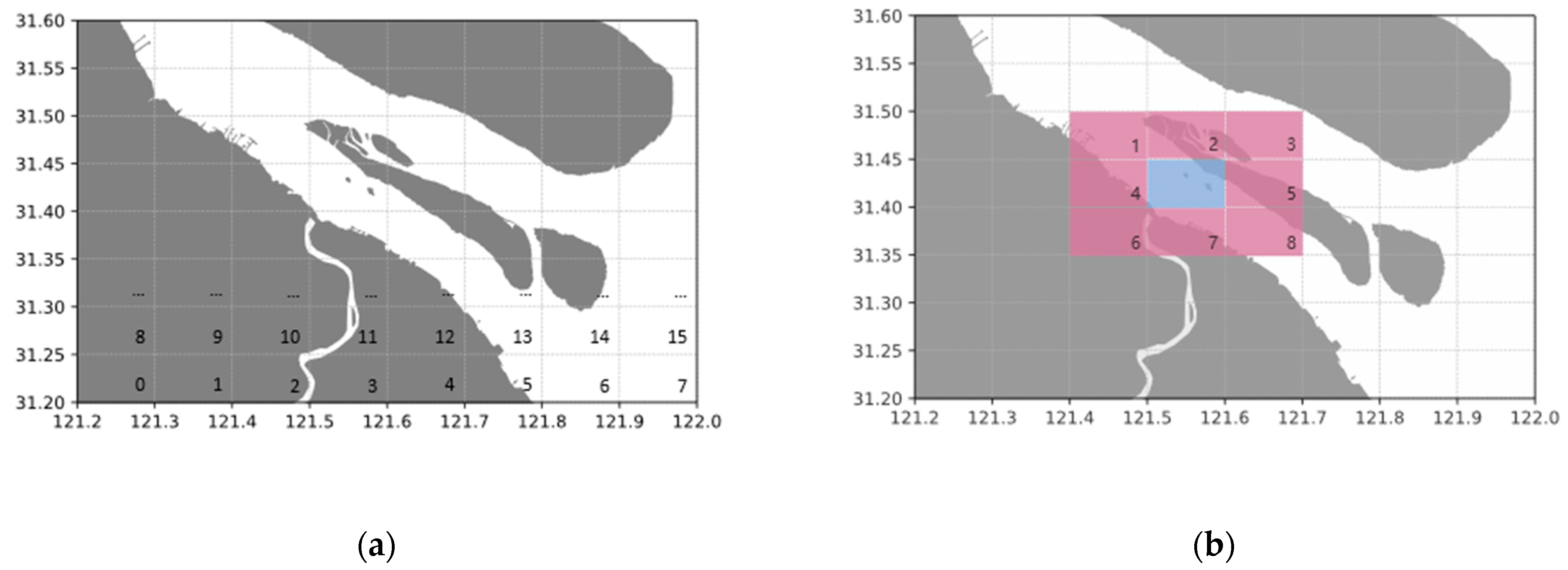
In this paper, the minimum latitude and longitude of the study area were set as the origin, and the grid index was incremented in the order of longitude direction first and then latitude direction, starting from 0. Figure 2a shows an illustrative diagram of dividing the region into equal-sized grids, with the index of each grid marked in the lower right corner. The model identifies a virtual grid using its assigned index and uses the geographical center of the grid as a feature of the grid. Because the virtual grid is a rectangle of equal size, the geographical center can easily be obtained as the center point of the grid rectangle. After dividing the spatial grid, the number of trajectory position points appearing in each grid is counted and used as a feature in subsequent analyses.

4.1.2. Spatial Embedding Pre-Training

After completing the grid partitioning, spatial adjacency structure pre-training was performed on the partitioned grids to obtain embeddings of the intrinsic spatial relationships within the grids. These embeddings are used to incorporate the spatial structural dependencies into the construction of the next-step hierarchical heterogeneous graph features. Specifically, first, a pre-training spatial relationship graph is established to model the spatial dependencies of the grids. A set of nodes N s p a t is established for the spatial dependency graph, consisting of N g r i d spatial grids. For any virtual grid u N s p a t , the spatial eight-neighborhood of the grid is calculated and obtained. Using the spatial eight-neighborhood as the grid neighborhood N s ( u ) , bidirectional edges u , n i , n i , u , n i N s ( u ) are created between the current grid and each of its eight neighbors. The edges in the spatial dependency relationship edge set E s p a t are then formed by adding the self-loop edge u , u to the set of edges, and the spatial dependency graph can be established as G =   ( N s p a t , E s p a t ) :
E s p a t = u N s p a t n i N s ( u ) u , n i
This can ensure that all trajectories entering the grid from adjacent grids have their internal associative relationships between the partitioned grids learned by the model, thus explicitly modeling the spatial dependency structure of the spatially related grids. As shown in Figure 2b, the blue represents the current virtual grid and the pink represents the eight-neighborhood of the grid in establishing spatial adjacency relationships, thus forming a pre-training spatial structural relationship. Afterward, using the coordinates of virtual grid center points as features, the node neighborhoods of the pre-trained spatial dependency graph are explored through methods such as node2vec [29], and embeddings are iteratively learned to obtain node representations that contain spatial structural dependency information. After pre-training f s p a t = n o d e 2 v e c (G), f s p a t R N g r i d × d can be obtained, where f s p a t is the generated embedding and d is the dimension size of the intermediate layer embedding in the model; the representations of each virtual grid node obtained can then be used as one of the node features for constructing heterogeneous graph features in a hierarchical structure.

4.2. Hierarchical Heterogeneous Graph Construction

4.2.1. Hierarchical Heterogeneous Graph Structure Construction

After completing the virtual grid spatial dependency pre-training, hierarchical heterogeneous graphs were separately constructed for each trajectory. The heterogeneous graph of the AISim model is divided into two parts according to different levels, namely the real trajectory position points and the constructed virtual nodes. Since similar trajectory position points may be mapped to the same or adjacent virtual grids, that is, several real trajectory points’ information is aggregated into the same structure content, from the perspective of signal processing this operation can be regarded as irregularly downsampling the trajectory points. Therefore, the real trajectory points and their corresponding virtual grids constitute different levels of signal feature extraction, and thus the proposed model introduces the concept of hierarchy.
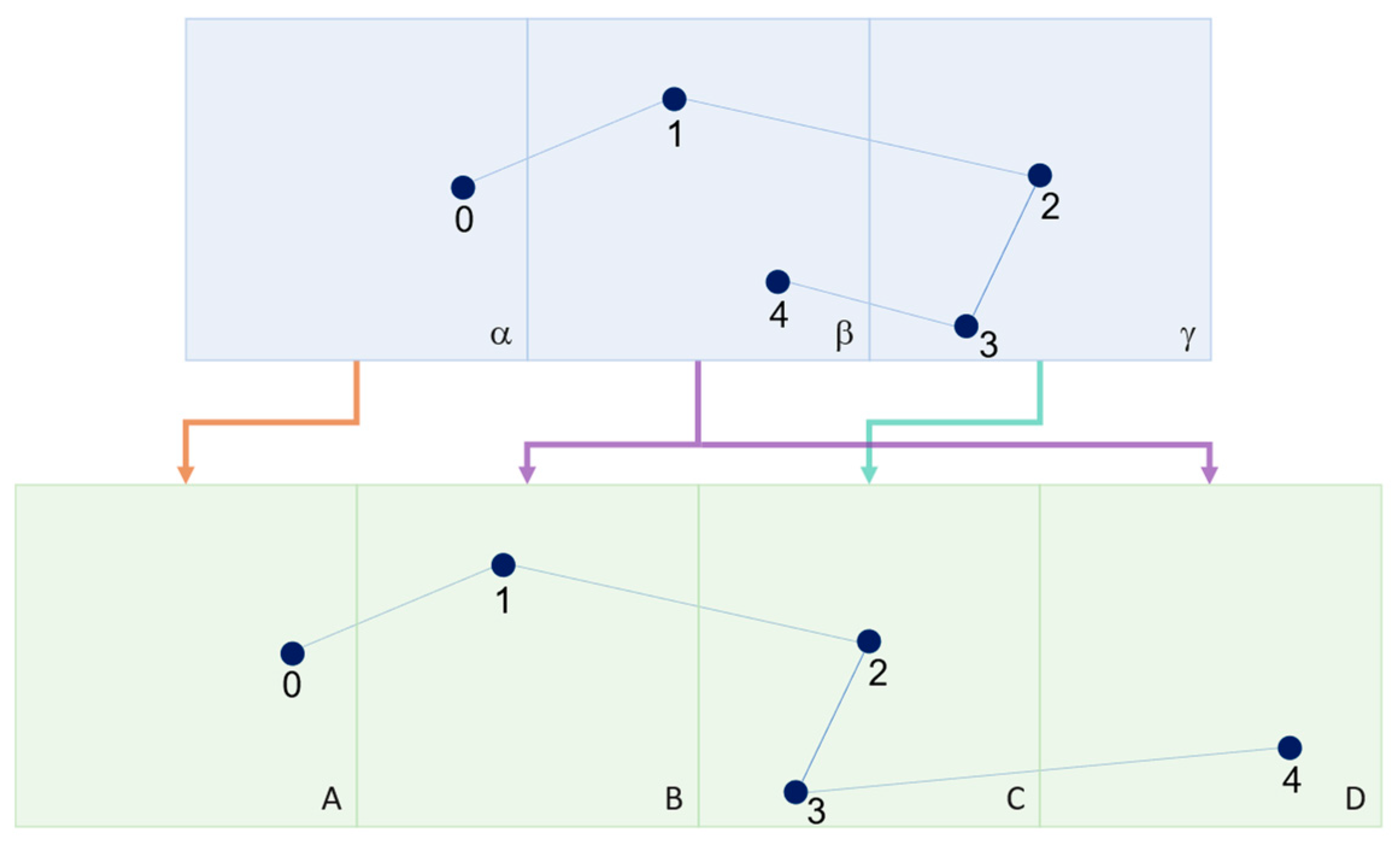
The first level is the construction of virtual grids. Given a real vessel’s latitude and longitude coordinate trajectory, for each recorded real position it is assigned to a spatial virtual grid corresponding to the geographically divided regions under each virtual grid in Section 4.1, that is, each real trajectory point is allocated to a virtual grid. It should be noted that the virtual grid assigned to each real trajectory point is not exactly the same as the spatial grid partitioned in Section 4.1. In fact, the virtual grid in this section uses the center position point of the spatial grid in Section 4.1 as a feature and adds sequence features to form a new virtual grid. This is because the trajectory may pass through the same spatial grid repeatedly. For a trajectory, passing through the same area does not necessarily mean that all virtual grids corresponding to the trajectory segment in this locality have the same features, but only the same spatial features. If virtual grids are constructed only based on spatial features, the sequential dependence information will be lost. Therefore, the AISim virtual grid construction module follows the spatial virtual grids partitioned in Section 4.1 and adds sequential information based on them to derive different sequential virtual grids. Sequential virtual grids derived from the same spatial virtual grid have the same spatial information and features, but their sequential features are different. More specifically, the hierarchical heterogeneous graph construction module first maps the real position points of this trajectory to the grid on space and generates a spatial grid sequence with the same length as the trajectory position points. During the process of traversing this spatial grid sequence from start to finish, the spatial virtual grids that are not connected are set as different sequential virtual grids, while the connected ones are set as the same sequential virtual grids. For example, as shown in Figure 3, assuming there is a trajectory with five positions indexed as 0, 1, 2, 3, and 4, distributed in three adjacent spatial grids α, β, and γ, the trajectory departs from α, passes through β and γ, and then folds back to β. The corresponding spatial grid sequence for this trajectory is αβγγβ, and the corresponding sequential virtual grid sequence is ABCCD. It can be seen that the correspondence between the spatial grid and the sequential grid is A → α, B → β, C → γ, D → β, where the → symbol indicates derivation. After obtaining the sequential virtual grids corresponding to the trajectory, the complete set of the virtual grid in the hierarchy is obtained.
Using the sequential virtual grids obtained from the previous steps as the type of grid nodes to be constructed in the heterogeneous graph, AISim connects the neighboring nodes of two types, sequential neighbors and spatial neighbors, to obtain a heterogeneous target trajectory graph. Assuming that there is a sequential virtual grid node, for sequence neighbors, according to the sequential virtual grid sequence obtained above, the N s e q sequential virtual grids adjacent to the front or back of the grid nodes are added to the sequence neighbor set. Here, N s e q is a manually set hyperparameter. For spatial neighbors, the spatial neighbors of the virtual grid to which the sequential virtual grids belong derive all sequential virtual grid sets in the part that the trajectory passes through and set them as spatial neighbors. Taking the union of the sequential neighbor set and the spatial neighbor set mentioned above, the entire neighbor set of the virtual grid node is obtained, and bidirectional edges are established between each node and its neighbors, plus self-edges. In this way, all edge adjacency relationships of the node are obtained. The above operations are performed on all sequential virtual grid nodes in the heterogeneous graph, and the full picture of the virtual grid node hierarchy is finally generated. Figure 4 shows the process of connecting sequential virtual grids to virtual grid hierarchical edges generated in Figure 3 (excluding self-edges). The spatial neighbors in the first figure and the sequence neighbors in the second figure are combined to generate the complete edge links in the third figure. Since there is currently only one hierarchy in the graph, that is, one type of node, and only one type of edge, the heterogeneous trajectory graph is temporarily a homogeneous graph.
The second level involves constructing the real trajectory positions of the recorded trajectory, forming a complete heterogeneous graph based on the first level. As shown in Figure 3, after generating a sequence of sequential virtual grids, all adjacent trajectory points located in the same spatial virtual grid are assigned to the same sequential virtual grid based on their correspondence with the sequential virtual grid. In this way, a batch of real trajectory position points that enter the same grid at the same time belong to the same sequential virtual grid, and thus share the spatial and sequential features of the sequential virtual grid. Finally, all real position points in the trajectory are used to generate a real position hierarchy node, and a unidirectional edge is created between the position hierarchy node and the virtual grid node based on the correspondence between the real position point and its corresponding sequential virtual grid. It should be noted that this article chooses to construct unidirectional edges because the AISim neural network graph module only aggregates information from the real position point hierarchy to the virtual grid hierarchy but does not update information from the virtual grid to the real location points. Whether updating information from the virtual grid to the real position point affects the representation learning of trajectory spatial features remains to be studied in future research and is not discussed further in this article.

4.2.2. Hierarchical Heterogeneous Graph Feature Construction

After generating the heterogeneous graph structure, the next step is to generate different feature combinations for the two types of nodes. For a heterogeneous hierarchical graph G = ( N , E ) generated from a trajectory T , AISim chooses to use four types of feature representations to characterize the sequence of virtual grid hierarchical nodes, which are the center point position of the grid f g c e n t , the sequence embedding of the grid f g s e q , the pre-trained embedding of the grid space f g s p a t , and the number of real trajectory positions contained in the grid f g n p o s . Next, we will introduce the sources and construction methods of each feature.
The construction of the grid center point position feature f g c e n t consists of feature acquisition and dimension transformation. The input feature of the grid center point position is composed of the coordinates of the center points of the spatial virtual grids corresponding to the virtual grid nodes in the heterogeneous graph. The sequential virtual grid nodes derived from the same spatial virtual grid share the same center point latitude and longitude position features. Since the input coordinate features have only two dimensions and do not match the dimensions of the model intermediate layer, an MLP is used to map the features to the dimensions of the model’s intermediate layer d :
f g c e n t = M L P X g c e n t , X g c e n t = X 1 g c e n t , , X u g c e n t , , X L g g c e n t
where f g c e n t R L g × d , X g c e n t R L g × 2 , X u g c e n t = ( l o n u , l a t u ) , and l o n u , l a t u represent the longitude and latitude of the u -th node in the spatial grid. After being mapped by MLP, each center location feature is dimensionally increased to d , f g c e n t R L g × d , followed by adding non-linear activation functions such as ReLU [30,31] for the mapping.
The grid sequence embedding f g s e q is obtained by sequentially encoding the center feature of the center positions in a single-layer bidirectional GRU [32] module in order to capture the sequential features of the grid sequences that the trajectory passes through:
f g s e q = B i G R U X g c e n t B i G R U X g c e n t , X g c e n t R L g × 2
where f g s e q R L g × d , X g c e n t represents the spatial grid longitude and latitude from the previous section and ⊕ denotes the tensor concatenation symbol. The center feature of the grid sequence can be seen as a low-resolution trajectory obtained by downsampling the original trajectory, and adding GRU to extract sequence features can significantly preserve the positional information of the original trajectory in a more robust way within the learned embedding. Additionally, since the forward and backward directions of the sequence may reflect different sequence information, both directions are modeled here to extract sequence features, with each direction generating a dimension of d / 2 ; the two output tensors are concatenated along the model dimension.
The grid spatial pre-training embedding f g s p a t is first obtained by the spatial dependencies of the spatial virtual grid in the first module embedding pre-training:
f s p a t = n o d e 2 v e c ( G ) ,   G = ( N s p a t , E s p a t )
obtaining f s p a t R N g r i d × d , where f s p a t is the pre-trained generated embedding, and then allocating spatial virtual grids to sequential virtual grids:
f g s p a t = M a p f s p a t , f s p a t R N g r i d × d
Finally, the spatial pre-training features f g s p a t R L g × d for each sequential virtual grid are obtained.
The number of real trajectory positions contained in the grid, denoted as f g n p o s , also belongs to spatial information. It is a statistical feature used to add class weight information to spatial grids, in order to characterize the possible importance of spatial grids within the region. In the first module, after partitioning the spatial virtual grids, the frequency information for the appearance of real trajectory position points in the training set is collected and counted. To maintain dimension alignment, an MLP mapping is also applied to the frequency information:
f g c e n t = M L P X g n p o s , X g n p o s R L g × 1
obtaining f g n p o s R L g × d .
After the construction of node features in the virtual grid hierarchy, the position feature X g c e n t is replaced by the coordinate feature X p c o o r d of the trajectory point. Referring to Equations (2) and (3), the hierarchical node coordinate feature f p c o o r d and sequence feature f p s e q of the trajectory position points can similarly be obtained by
f p c o o r d = M L P X p c o o r d , X p c o o r d R L g × 2
f p s e q = B i G R U X p c o o r d B i G R U X p c o o r d , X p c o o r d R L g × 2
where f p c o o r d R L g × d , f p s e q R L g × d .

4.3. Hierarchical Heterogeneous Graph Neural Network

Once the feature construction of all node types in the heterogeneous graph is completed, features can be entered into the heterogeneous graph neural network and representation learning for trajectories can be performed. It is particularly important to capture the dependency structure in vessel trajectories in order to find key information in the trajectory signal and learn the best feature representation for similarity measurement. AISim chooses a heterogeneous graph neural network model to perform feature fusion and information updating on two hierarchical nodes in the heterogeneous graph. As described in the previous section, AISim’s graph construction module considers the spatial and sequential dependencies of trajectories as homogeneous virtual node links and performs the same computation. Therefore, the heterogeneous graph constructed by AISim is a heterogeneous graph with two types of nodes and a single type of link.
To perform an information update across different node types, it is first necessary to be able to fuse different feature types within the same node type. Inspired by Zhang et al. [33], AISim uses BiGRU to fuse different features of the same dimension, forming a fusion feature with comprehensive expression capability across multiple feature types. Formally, for a constructed heterogeneous graph G = N , E , X = [ X N g , X N P ] , X N g = f g c e n t , f g s e q , f g s p a t , f g n p o s , and X N P = [ f p c o o r d , f p s e q ] , where X N g , X N P are the feature sets of grid and position type nodes, respectively. For a node u N in G , its features can be fused according to the following formula:
f u = i C u [ B i G R U { X i } B i G R U X i ] | F u |
where f u R d , F u represents the set of feature types for node u, and | F u | represents the number of elements in the feature type set. In the GRU, different feature types are treated as different step sizes in a sequence. The sequence outputs of each feature at each step are obtained by passing them through the GRU and concatenating them along the dimension of the output representation. The resulting representation is then averaged, and both types of nodes obtain the fusion feature using Equation (9).
After obtaining the fused features, information updates between heterogeneous nodes of different types are possible. In the heterogeneous graph neural network of AISim, a layer of graph neural network operation is performed, and the resulting representation is aggregated using the following Equation (10):
h d s t l + 1 = A G G r T E G N N G r , h r s r c l , h r d s t l , r s r c N , d s t = r d s t N g
where h r s r c l and h r d s t l are the input representation matrices for source nodes and destination nodes, respectively, whose information is aggregated under relation r in the l -th layer of the neural network. Here, T E = 1 , which means that there is only one type of edge. Since AISim has only unidirectional edges from location point nodes to grid nodes, i.e., the representation of location point nodes will not be updated by messages from grid nodes, r d s t N g , where N g is the set of grid-type nodes; all nodes can send messages outward, so r s r c N , where N is the set of all types of nodes. When l = 0 , h s r c l = f u , h d s t l = f v , u N , and v N g . G N N is a type of homogeneous graph neural network [34,35], and in this case, AISim uses a graph convolutional layer [36]. Finally, A G G is a certain aggregation function, such as taking the average or maximum value, but since the proposed model only has one type of edge, A G G does not have any effect in this case. It can be seen that AISim propagates the features of position nodes to grid nodes. Grid nodes receive shared information from position point neighbors, grid neighbors, and themselves, and update their own features. In this way, grid nodes not only aggregate the information of their corresponding position points but also transmit their own features to spatial and sequential neighboring grids, capturing spatial and sequential dependencies. The graph neural network module of AISim performs four graph convolution operations. The first heterogeneous graph convolution aggregates the information of the two types of nodes, transferring the position point information to the grid nodes for updating. The second convolution passes the message from grid nodes to neighbors based on the aggregated information of the two types of nodes. The third convolution aggregates position point information once again based on the node representation obtained in the second convolution, ensuring that the node information is not excessively lost and can be regarded as a form of residual connection. The fourth convolution passes the message to neighboring nodes again, further capturing spatial dependencies. After completing the graph convolution, a graph attention layer [37] is applied to grid type nodes to capture key grid objects and output node representations with multiple attention heads. Finally, the node readout function based on BiGRU reads all grid node representations as the representation of the entire heterogeneous hierarchical graph, obtaining the embedding of the trajectory representation.
After obtaining embeddings that represent two trajectories, the Euclidean distance is used to calculate the distance between the two embedding vectors. The difference between the resulting distance and the precise distance of the trajectory calculation result is used as the error signal, which can be backpropagated to guide the network parameter update. This allows the model to learn the given similarity measure.

5. Experiments and Discussion

To validate the effectiveness and evaluate the performance of the proposed AISim framework, extensive experiments were conducted on two large real trajectory datasets. Two similarity measures based on different concepts, DTW and discrete Fréchet distance, were used to test AISim on each dataset, and a key hyperparameter of the model was experimentally tested under different settings. Finally, a comparative experiment was conducted on two advanced-sequence neural network models, TCN [38] and transformer [39], under the same experimental setting. The performance of AISim under the Top-K similarity search metric demonstrated the effectiveness of the proposed model.

5.1. Experimental Settings

5.1.1. Data Description

In order to verify the performance of the model, two trajectory datasets were used for experiments in this paper. The first one was the publicly available Porto taxi GPS trajectory dataset [40,41], and the second was the vessel AIS trajectory data for Wusongkou (WSK) in Shanghai, China (data source: HiFleet, www.hifleet.com, accessed on 22 November 2022). Illustration of raw WSK trajectories after data cleaning is shown in Figure 5. All trajectories underwent necessary preprocessing, including removal of trajectory drift, AIS signal content that does not conform to IMO specifications, etc. [20,21,22,42]. Ten thousand trajectories were selected from Porto, with a length range from 100 to 1000 positions; five thousand trajectories were selected from WSK, with a length range from 100 to 400 positions. By experimenting with diverse source trajectory data, the generality of the proposed AISim framework was demonstrated. After obtaining preprocessed trajectories, trajectories were generated by computing pairwise distances between trajectories using DTW and discrete Fréchet distance. As DTW is asymmetric, the method of adding the DTW metric and its reverse direction symmetrically was adopted here.

5.1.2. Evaluation Metrics

This article evaluates the performance of the proposed model on the Top-K similarity search task using three metrics: HR@10, HR@50, and R10@50. These represent the hit rate at the top 10 and top 50 predictions, as well as the recall rate of the top 10 true values within the top 50.

5.1.3. Parameter Settings

In addition to the number of grids under study, AISim has several key parameters as listed in Table 1.
Note that the dimensions of all intermediate and output layers of the model, which equals the model embedding size, are 64. In addition, 70% of the trajectories and their ad-hoc distances were used for training, and the remaining 30% were used for validation.
In addition to the special parameters of the model architecture, the experiment ensured that the hyperparameters of the baseline model were basically consistent to control the conditions of the control experiment as much as possible.

5.2. Results

Table 2 shows the performance of AISim and the control model on the Top-K similarity search task; the bold font indicates the best results.
From Table 2, it can be seen that both TCN and transformer, as advanced sequence models, have their own strengths in various indicators, especially HR10, while AISim outperforms the control model on almost all metrics. Taking the Fréchet distance of the Porto dataset that models perform most equally on as an example, the performance of TCN and transformer on the HR10 and HR50 metrics is basically similar, while AISim surpasses them by 15% on HR10; in the Fréchet distance of WSK where it has the greatest advantage, AISim outperforms the relatively good TCN by 66% on HR10. It shows that AISim successfully captures the intrinsic spatial structural relationship within trajectories and can learn reasonable trajectory representations better than pure sequence models.
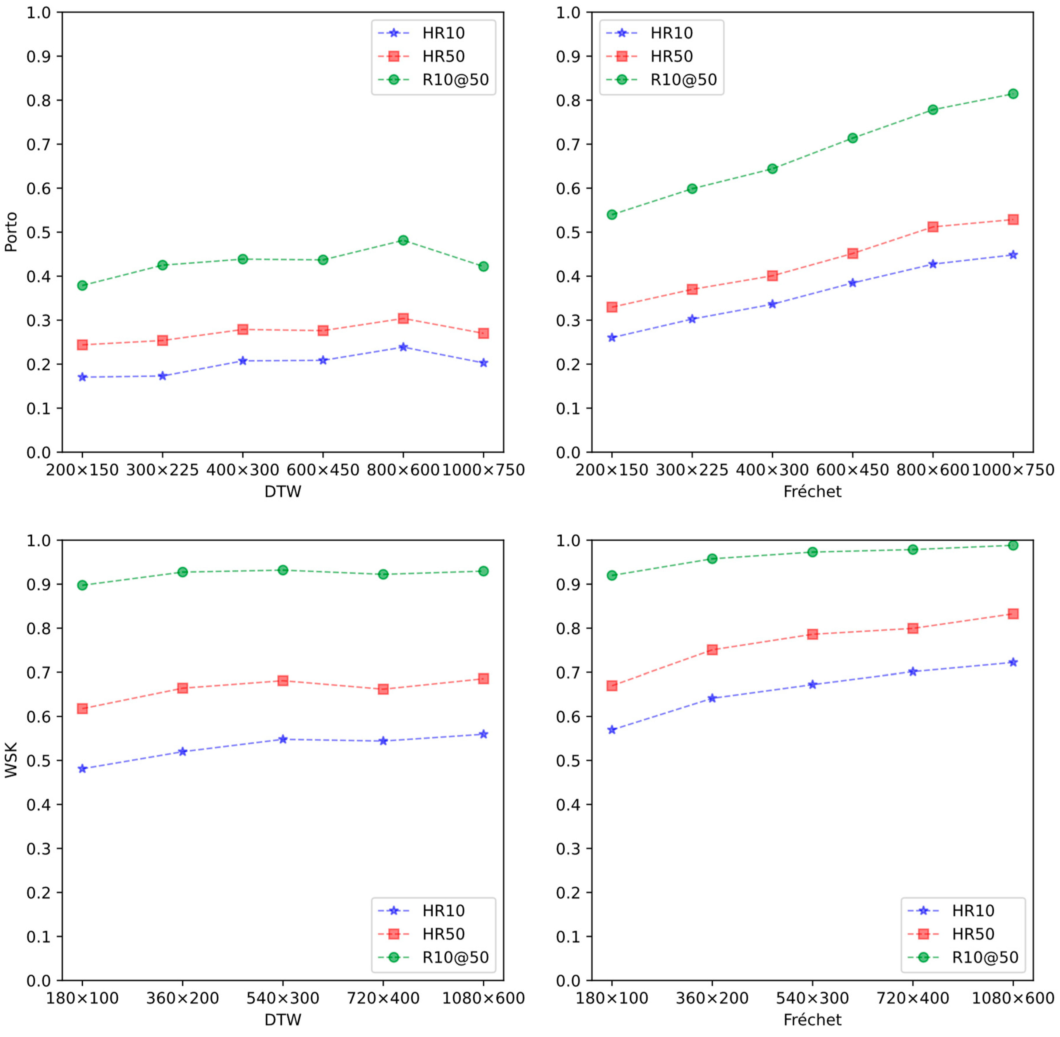
Figure 6 provides a clearer and more intuitive observation of the different performances exhibited by the models.
After comparison with the baseline model, Figure 7 shows the impact of a key parameter of the AISim model, the number of grids, on its performance.
This article assumes that a square grid shape is most likely to have the best effect, so the ratio of longitude and latitude of the grid is set according to the closest integer ratio of longitude and latitude in research area A. For Porto and WSK, six and five parameter pairs, respectively, were selected for experimentation. First, the most intuitive trend that can be observed is that as the number of grids increases, overall model performance shows an upward trend, but bigger is not always better.

5.3. Discussion

The first model comparison experiment in Section 5.2 verified the effectiveness of the AISim model and also indicated that different models may perform differently on different distance metrics, but it is still possible to use a single model to learn many metrics as well as possible, which is a problem worth continuing work on. Secondly, the same distance metric shows significant differences in performance on different datasets, which may have two possible reasons. The first reason is the difference in trajectory length selection after preprocessing, which needs further investigation in future studies. The second possible reason is the difference in inherent data characteristics of the dataset. By visualizing trajectories, it can be found that the Porto dataset has features such as large trajectory changes, many curve bends, and low approximation compared to WSK, which has the characteristics of small trajectory changes, few curve bends, and high approximation as a vessel AIS trajectory. This reflects the uniqueness of similarity research on vessel trajectories.
In the second parameter comparison experiment, different distance functions of the Porto dataset showed different trends with parameter changes. For example, in the Porto dataset, the DTW metric achieved the best performance at a resolution of 800 × 600, while the Fréchet distance achieved the best effect at a maximum resolution of 1000 × 750. This indicates that different distance functions require different downsampling resolutions for trajectories. Therefore, using adaptive grid resolutions for different distance metrics may be a future research focus. In addition, by observing the trend differences of different metrics on parameter effects in the two datasets, it can be found that the Fréchet distance is more sensitive to parameters and may show excessive damage to key information in the Fréchet distance due to excessive downsampling. Future research can focus on how to preserve key information.

6. Conclusions

Vessel trajectory similarity measurement is a fundamental issue in maritime regulation and smart shipping. This article proposes a vessel trajectory similarity measurement framework based on heterogeneous graph networks to fit any distance metric, reducing the cost of vessel trajectory similarity measurement. The framework first constructs a spatial structure for the research area based on the dataset and extracts spatial features to form a spatial pre-training graph. Then, a space-dependent extraction method based on random walks is used to pre-train the spatial pre-training graph. In the second step, the trajectories are constructed into graphs, with heterogeneous graph neighbors connected by spatial and sequential neighbors in grid and positional points, and relevant features are constructed. Then, the proposed heterogeneous graph neural network learns the representation of the entire graph through five layers of information propagation and feature mapping, and finally optimizes the entire model through metric learning to transfer the real signal and learn the closest original distance metric. Experiments on two datasets show that the proposed framework has a performance improvement of 5% to 66% compared to advanced learning-based sequence models, confirming the effectiveness of the proposed framework. Possible reasons for the experimental results are discussed, and future research directions, such as adaptive grid granularity and spatial key feature recognition, are explored.

Author Contributions

Conceptualization, S.L. and W.Z.; methodology, S.L.; software, S.L.; validation, S.L.; writing—original draft preparation, S.L.; writing—review and editing, W.Z. All authors have read and agreed to the published version of the manuscript.

Funding

This work was sponsored by the National Natural Science Foundation of China (Grants No. 61906117 and 31870979).

Data Availability Statement

The open Porto taxi dataset is available at: archive.ics.uci.edu/dataset/339/taxi+service+trajectory+prediction+challenge+ecml+pkdd+2015 accessed on 19 June 2023.

Conflicts of Interest

The authors declare no conflict of interest.

Nomenclature

NotationsMeanings
AStudy area within a given range
GSpatial structure pre-training graph A
N s p a t , E s p a t Node set and edge set of G
N l o n , N l a t , N g r i d Number of grid nodes in longitude, latitude, and total
TPre-processed trajectory dataset
T i i -th trajectory record
G i i -th trajectory hierarchical heterogeneous graph
N p Node set of real location points
N g Node set of virtual grid points
N = N p N g Set of both types of nodes
d Embedding dimension
A G G Aggregation function
h r s r c l , h r d s t l Representation of source and target node at the l -th layer under relationship r
T E Set of edge type E

References

  1. Mao, S.; Tu, E.; Zhang, G.; Rachmawati, L.; Rajabally, E.; Huang, G.-B. An Automatic Identification System (AIS) Database for Maritime Trajectory Prediction and Data Mining. In Proceedings of ELM-2016; Springer International Publishing: Berlin/Heidelberg, Germany, 2016. [Google Scholar]
  2. Tu, E.; Zhang, G.; Rachmawati, L.; Rajabally, E.; Huang, G.-B. Exploiting AIS Data for Intelligent Maritime Navigation: A Comprehensive Survey From Data to Methodology. IEEE Trans. Intell. Transp. Syst. 2018, 19, 1559–1582. [Google Scholar] [CrossRef]
  3. Pallotta, G.; Vespe, M.; Bryan, K. Traffic Knowledge Discovery from AIS Data. In Proceedings of the 16th International Conference on Information Fusion, Istanbul, Turkey, 9–12 July 2013; pp. 1996–2003. [Google Scholar]
  4. Munim, Z.H.; Dushenko, M.; Jimenez, V.J.; Shakil, M.H.; Imset, M. Big Data and Artificial Intelligence in the Maritime Industry: A Bibliometric Review and Future Research Directions. Marit. Policy Manag. 2020, 47, 577–597. [Google Scholar] [CrossRef]
  5. Yang, D.; Wu, L.; Wang, S.; Jia, H.; Li, K.X. How Big Data Enriches Maritime Research—A Critical Review of Automatic Identification System (AIS) Data Applications. Transp. Rev. 2019, 39, 755–773. [Google Scholar] [CrossRef]
  6. Shelmerdine, R.L. Teasing out the Detail: How Our Understanding of Marine AIS Data Can Better Inform Industries, Developments, and Planning. Mar. Policy 2015, 54, 17–25. [Google Scholar] [CrossRef]
  7. Li, H.; Liu, J.; Liu, R.; Xiong, N.; Wu, K.; Kim, T. A Dimensionality Reduction-Based Multi-Step Clustering Method for Robust Vessel Trajectory Analysis. Sensors 2017, 17, 1792. [Google Scholar] [CrossRef] [Green Version]
  8. Zhang, D.; Zhang, Y.; Zhang, C. Data Mining Approach for Automatic Ship-Route Design for Coastal Seas Using AIS Trajectory Clustering Analysis. Ocean Eng. 2021, 236, 109535. [Google Scholar] [CrossRef]
  9. Li, H.; Liu, J.; Yang, Z.; Liu, R.W.; Wu, K.; Wan, Y. Adaptively Constrained Dynamic Time Warping for Time Series Classification and Clustering. Inf. Sci. 2020, 534, 97–116. [Google Scholar] [CrossRef]
  10. Cao, J.; Liang, M.; Li, Y.; Chen, J.; Li, H.; Liu, R.W.; Liu, J. PCA-Based Hierarchical Clustering of AIS Trajectories with Automatic Extraction of Clusters. In Proceedings of the 2018 IEEE 3rd International Conference on Big Data Analysis (ICBDA), Shanghai, China, 9–12 March 2018; pp. 448–452. [Google Scholar]
  11. Wei, Z.; Xie, X.; Lv, W. Self-Adaption Vessel Traffic Behaviour Recognition Algorithm Based on Multi-Attribute Trajectory Characteristics. Ocean Eng. 2020, 198, 106995. [Google Scholar] [CrossRef]
  12. Yan, Z.; Yang, G.; He, R.; Yang, H.; Ci, H.; Wang, R. Ship Trajectory Clustering Based on Trajectory Resampling and Enhanced BIRCH Algorithm. J. Mar. Sci. Eng. 2023, 11, 407. [Google Scholar] [CrossRef]
  13. Zhang, Y.; Shi, G. Trajectory Similarity Measure Design for Ship Trajectory Clustering. In Proceedings of the 2021 IEEE 6th International Conference on Big Data Analytics (ICBDA), Xiamen, China, 5–8 March 2021; pp. 181–187. [Google Scholar]
  14. Pallotta, G.; Jousselme, A.-L. Data-Driven Detection and Context-Based Classification of Maritime Anomalies. In Proceedings of the 2015 18th International Conference on Information Fusion (Fusion), Washington, DC, USA, 6–9 July 2015; pp. 1152–1159. [Google Scholar]
  15. Zhang, B.; Hirayama, K.; Ren, H.; Wang, D.; Li, H. Ship Anomalous Behavior Detection Using Clustering and Deep Recurrent Neural Network. J. Mar. Sci. Eng. 2023, 11, 763. [Google Scholar] [CrossRef]
  16. Karataş, G.B.; Karagoz, P.; Ayran, O. Trajectory Pattern Extraction and Anomaly Detection for Maritime Vessels. Internet Things 2021, 16, 100436. [Google Scholar] [CrossRef]
  17. Li, H.; Lam, J.S.L.; Yang, Z.; Liu, J.; Liu, R.W.; Liang, M.; Li, Y. Unsupervised Hierarchical Methodology of Maritime Traffic Pattern Extraction for Knowledge Discovery. Transp. Res. Part C Emerg. Technol. 2022, 143, 103856. [Google Scholar] [CrossRef]
  18. Tao, Y.; Both, A.; Silveira, R.I.; Buchin, K.; Sijben, S.; Purves, R.S.; Laube, P.; Peng, D.; Toohey, K.; Duckham, M. A Comparative Analysis of Trajectory Similarity Measures. GIScience Remote Sens. 2021, 58, 643–669. [Google Scholar] [CrossRef]
  19. Itakura, F. Minimum Prediction Residual Principle Applied to Speech Recognition. IEEE Trans. Acoust. Speech Signal Process. 1975, 23, 67–72. [Google Scholar] [CrossRef]
  20. Lee, W.; Cho, S.-W. AIS Trajectories Simplification Algorithm Considering Topographic Information. Sensors 2022, 22, 7036. [Google Scholar] [CrossRef]
  21. Yan, R.; Mo, H.; Yang, D.; Wang, S. Development of Denoising and Compression Algorithms for AIS-Based Vessel Trajectories. Ocean Eng. 2022, 252, 111207. [Google Scholar] [CrossRef]
  22. Zhao, L.; Shi, G.; Yang, J. Ship Trajectories Pre-Processing Based on AIS Data. J. Navig. 2018, 71, 1210–1230. [Google Scholar] [CrossRef]
  23. Yao, X.U.; Zhuoran, L.I.; Jinlong, M.; Lipo, Z.; Jianxin, W.E.N.; Guiling, W. Extraction Method of Marine Lane Boundary from Exploiting Trajectory Big Data. J. Comput. Appl. 2019, 39, 105. [Google Scholar] [CrossRef]
  24. Yao, D.; Zhang, C.; Zhu, Z.; Hu, Q.; Wang, Z.; Huang, J.; Bi, J. Learning Deep Representation for Trajectory Clustering. Expert Syst. 2018, 35, e12252. [Google Scholar] [CrossRef]
  25. Zhao, L.; Shi, G. A Novel Similarity Measure for Clustering Vessel Trajectories Based on Dynamic Time Warping. J. Navig. 2019, 72, 290–306. [Google Scholar] [CrossRef]
  26. Šakan, D.; Žuškin, S.; Rudan, I.; Brčić, D. Container Ship Fleet Route Evaluation and Similarity Measurement between Two Shipping Line Ports. J. Mar. Sci. Eng. 2023, 11, 400. [Google Scholar] [CrossRef]
  27. Lu, N.; Liang, M.; Yang, L.; Wang, Y.; Xiong, N.; Liu, R.W. Shape-Based Vessel Trajectory Similarity Computing and Clustering: A Brief Review. In Proceedings of the 2020 5th IEEE International Conference on Big Data Analytics (ICBDA), Xiamen, China, 8–11 May 2020; pp. 186–192. [Google Scholar]
  28. Liang, M.; Liu, R.W.; Li, S.; Xiao, Z.; Liu, X.; Lu, F. An Unsupervised Learning Method with Convolutional Auto-Encoder for Vessel Trajectory Similarity Computation. Ocean Eng. 2021, 225, 108803. [Google Scholar] [CrossRef]
  29. Grover, A.; Leskovec, J. Node2vec: Scalable Feature Learning for Networks. In Proceedings of the 22nd ACM SIGKDD International Conference on Knowledge Discovery and Data Mining, San Francisco, CA, USA, 13–17 August 2016; Association for Computing Machinery: New York, NY, USA, 2016; pp. 855–864. [Google Scholar]
  30. Hahnloser, R.H.R.; Sarpeshkar, R.; Mahowald, M.A.; Douglas, R.J.; Seung, H.S. Digital Selection and Analogue Amplification Coexist in a Cortex-Inspired Silicon Circuit. Nature 2000, 405, 947–951. [Google Scholar] [CrossRef] [PubMed]
  31. Krizhevsky, A.; Sutskever, I.; Hinton, G.E. ImageNet Classification with Deep Convolutional Neural Networks. Commun. ACM 2017, 60, 84–90. [Google Scholar] [CrossRef] [Green Version]
  32. Cho, K.; van Merriënboer, B.; Gulcehre, C.; Bahdanau, D.; Bougares, F.; Schwenk, H.; Bengio, Y. Learning Phrase Representations Using RNN Encoder–Decoder for Statistical Machine Translation. In Proceedings of the 2014 Conference on Empirical Methods in Natural Language Processing (EMNLP), Doha, Qatar, 25–29 October 2014; Association for Computational Linguistics: Cambridge, MA, USA, 2014; pp. 1724–1734. [Google Scholar]
  33. Zhang, C.; Song, D.; Huang, C.; Swami, A.; Chawla, N.V. Heterogeneous Graph Neural Network. In Proceedings of the 25th ACM SIGKDD International Conference on Knowledge Discovery & Data Mining, Anchorage, AK, USA, 25 July 2019; Association for Computing Machinery: New York, NY, USA, 2019; pp. 793–803. [Google Scholar]
  34. Zhou, J.; Cui, G.; Hu, S.; Zhang, Z.; Yang, C.; Liu, Z.; Wang, L.; Li, C.; Sun, M. Graph Neural Networks: A Review of Methods and Applications. AI Open 2020, 1, 57–81. [Google Scholar] [CrossRef]
  35. Battaglia, P.W.; Hamrick, J.B.; Bapst, V.; Sanchez-Gonzalez, A.; Zambaldi, V.; Malinowski, M.; Tacchetti, A.; Raposo, D.; Santoro, A.; Faulkner, R.; et al. Relational Inductive Biases, Deep Learning, and Graph Networks. arXiv 2018, arXiv:1806.01261. [Google Scholar]
  36. Kipf, T.N.; Welling, M. Semi-Supervised Classification with Graph Convolutional Networks. arXiv 2017, arXiv:1609.02907. [Google Scholar]
  37. Veličković, P.; Cucurull, G.; Casanova, A.; Romero, A.; Liò, P.; Bengio, Y. Graph Attention Networks. arXiv 2018, arXiv:1710.10903. [Google Scholar]
  38. Bai, S.; Kolter, J.Z.; Koltun, V. An Empirical Evaluation of Generic Convolutional and Recurrent Networks for Sequence Modeling. arXiv 2018, arXiv:1803.01271. [Google Scholar]
  39. Vaswani, A.; Shazeer, N.; Parmar, N.; Uszkoreit, J.; Jones, L.; Gomez, A.N.; Kaiser, Ł.; Polosukhin, I. Attention Is All You Need. In Advances in Neural Information Processing Systems; Association for Computing Machinery: New York, NY, USA, 2017; Volume 30. [Google Scholar]
  40. Moreira-Matias, L.; Gama, J.; Ferreira, M.; Mendes-Moreira, J.; Damas, L. Predicting Taxi–Passenger Demand Using Streaming Data. IEEE Trans. Intell. Transp. Syst. 2013, 14, 1393–1402. [Google Scholar] [CrossRef] [Green Version]
  41. Moreira-Matias, L.; Gama, J.; Ferreira, M.; Mendes-Moreira, J.; Damas, L. Time-Evolving O-D Matrix Estimation Using High-Speed GPS Data Streams. Expert Syst. Appl. 2016, 44, 275–288. [Google Scholar] [CrossRef] [Green Version]
  42. Sang, L.; Wall, A.; Mao, Z.; Yan, X.; Wang, J. A Novel Method for Restoring the Trajectory of the Inland Waterway Ship by Using AIS Data. Ocean Eng. 2015, 110, 183–194. [Google Scholar] [CrossRef] [Green Version]
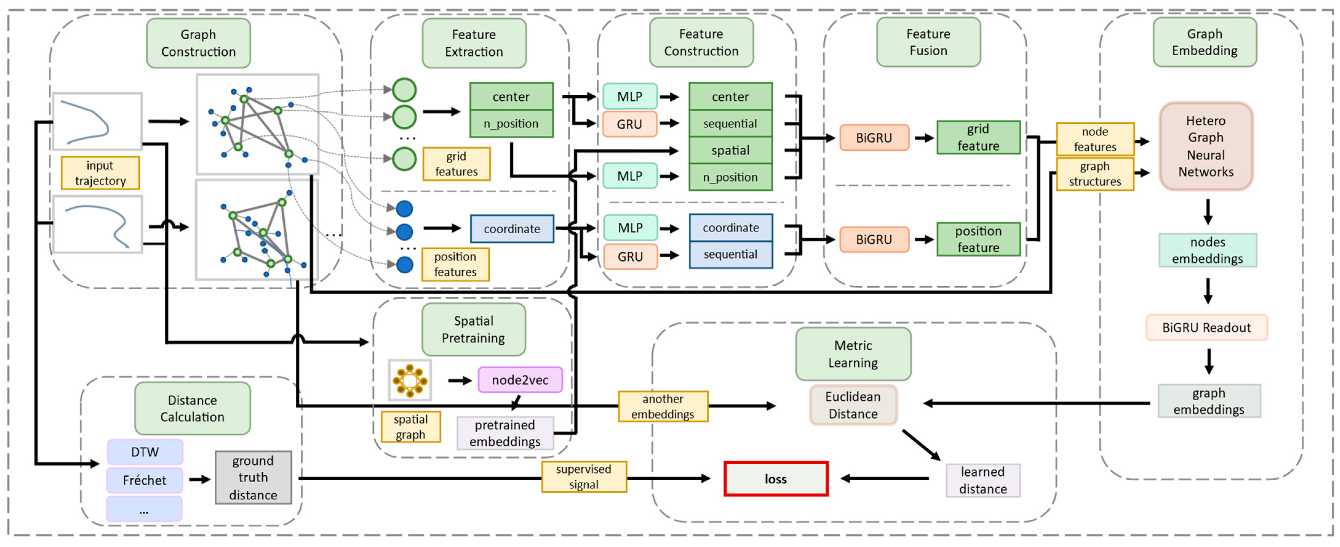
Figure 1. Overview of the proposed AISim framework.
Jmse 11 01318 g001
Figure 2. (a) Demonstration of spatial grid partitioning and indexing; (b) eight-neighborhood of a certain grid.
Jmse 11 01318 g002
Figure 3. Generation procedure of sequential virtual grids.
Jmse 11 01318 g003
Figure 4. Connection and combination of links in virtual grid hierarchy. Letters represents grid nodes.
Jmse 11 01318 g004
Figure 5. Raw vessel trajectories in Wusongkou, Shanghai.
Jmse 11 01318 g005
Figure 6. Illustration of performance comparison.
Jmse 11 01318 g006
Figure 7. Performance comparison under various N l o n   a n d   N l a t parameters.
Jmse 11 01318 g007
Table 1. Parameter settings in experiments.
ParametersValuesMeanings
N s e q 10Number of sequential neighbors
d 64Model embedding size
n _ s a m p l e 20Number of learning samples
Table 2. Performance comparison.
DatasetMethodDTWFréchet
HR10HR50R10@50HR10HR50R10@50
PortoTCN0.18280.27740.41160.38430.47800.7219
Transformer0.14890.25310.39310.38980.47750.7809
AISim0.23870.30390.48150.44840.52870.8145
WSKTCN0.35030.48930.75350.43450.52590.8251
Transformer0.40450.58430.84460.38110.57410.8511
AISim0.54800.68120.93190.72230.83260.9883
The bold indicate best performance.
Disclaimer/Publisher’s Note: The statements, opinions and data contained in all publications are solely those of the individual author(s) and contributor(s) and not of MDPI and/or the editor(s). MDPI and/or the editor(s) disclaim responsibility for any injury to people or property resulting from any ideas, methods, instructions or products referred to in the content.