For the numerical simulations conducted in the present study, the commercial CFD software STAR-CCM+ (version 15.06.007-R8) was employed. A trimmed hexahedral mesher with prism layers on the wall boundaries was employed in all the main types of simulations (towing resistance, propeller in open water, and ship self-propulsion calculations), as well as additional simulations with a flat plate, which were used to assess the influence of surface roughness height. All simulations, except for the flat plate calculations, were carried out in a time-dependent manner using the implicit unsteady segregated flow solver. Simulations involving rotating propeller (open water and self-propulsion) were performed using the sliding mesh technique to fully account for the interaction between the rotating and stationary components in the setup. The properties of water and air used in the simulations were derived from recorded values during the sea trials of MV REGAL. The simulations were performed for full-scale conditions corresponding to sea trials, as specified in the case description for the JoRes CFD Workshop regarding the MV REGAL vessel [
20]. Three ship speeds (9, 10.5, and 12 knots) were investigated in the resistance and self-propulsion scenarios, while in the open water case the advance coefficient (J) values of 0.2, 0.3, 0.4, 0.5, and 0.6 were used. The case-specific details of numerical setups are addressed for each individual simulation scenario in their respective subsections below.
A high-Reynolds near-wall treatment method was employed in the analyses. While using fine near-wall meshes with Y+ < 5 offers advantages in accurately predicting the frictional component of forces and moments, as well as modelling boundary layer separation/detachment, especially in Scale-Resolving Simulations, it becomes impractical in a full-scale case due to the excessively large mesh size and the small time step required to maintain the desired Courant number level in the areas of mesh refinement. In this regard, one needs to remember that it is not sufficient to increase mesh density only in the direction normal to the wall. Eddies developing in the near-wall region also require fine mesh resolution in the spanwise and streamwise directions. Failing to capture those eddies may compromise the overall simulation quality. Therefore, avoiding the resolution of viscous sub-layers may be a more reliable approach for solving high-Reynolds flows, even with such techniques as DES and LES. Another reason for choosing the high Y+ near-wall treatment is the inclusion of surface roughness, which relies on the use of roughness-modified wall functions. The present setup employs blended wall functions, supporting the so-called “All Y+ Treatment” method.
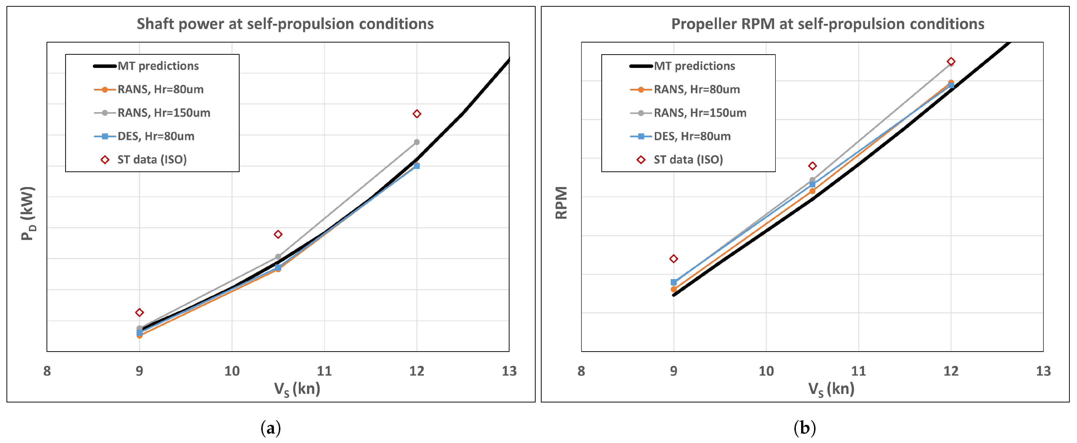
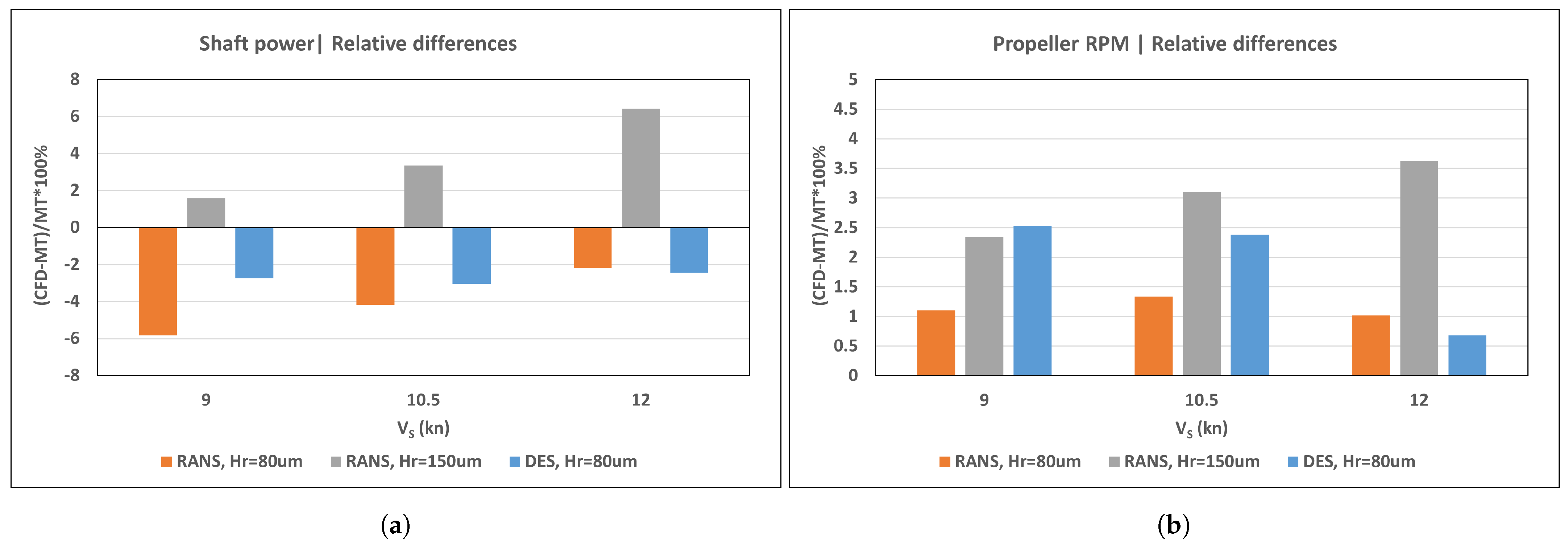
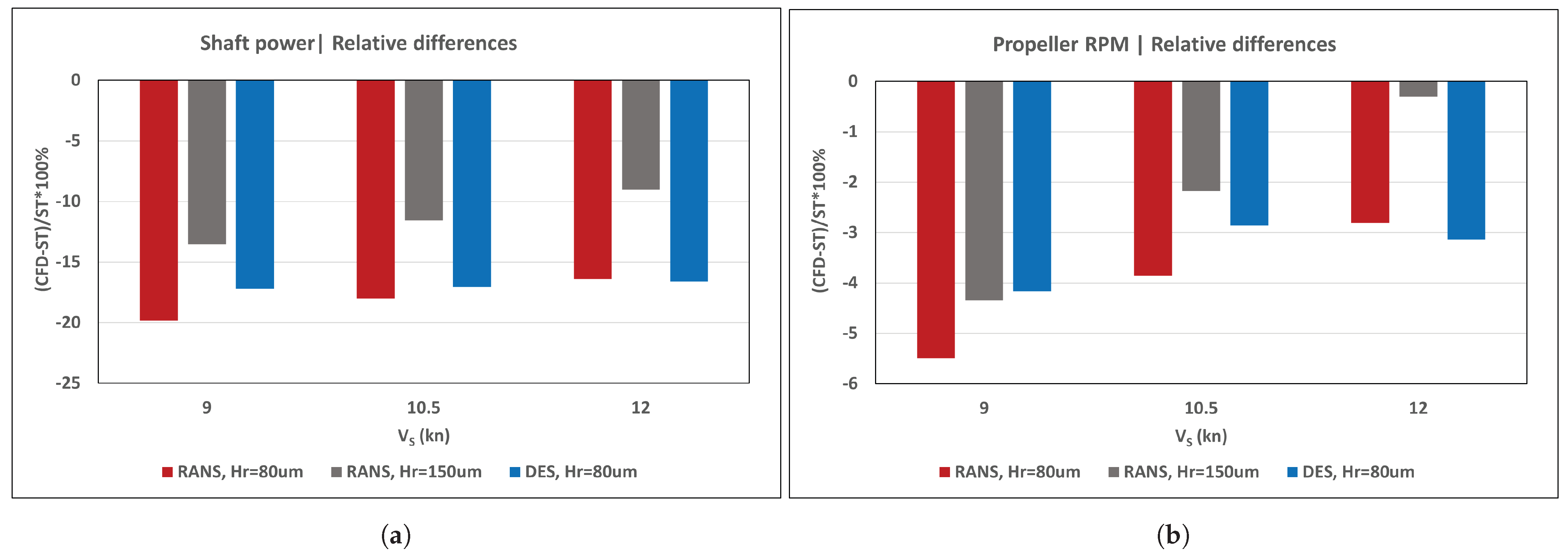
Separately, as a part of the JoRes project, SINTEF Ocean has conducted a model test campaign with the MV REGAL vessel. The campaign included towing resistance, open water, and propulsion tests in calm water at the scale of 1:23.111. The results of model tests were used in full-scale performance prediction for the sea trial conditions, following the standard procedure applied at SINTEF Ocean for single-screw ships [
21]. The results of performance prediction were compared against the sea trials data, which was post-processed according to the ISO15016 standard [
22], as well as the CFD calculations conducted at full-scale. The comparisons focused on propeller RPM and propeller shaft power, P
D. Additional comparisons were made between the CFD calculations and model test results extrapolated to full-scale conditions, examining the towing resistance of the ship, its dynamic position, and propeller characteristics in open water.
3.1. Open Water Propeller Simulations
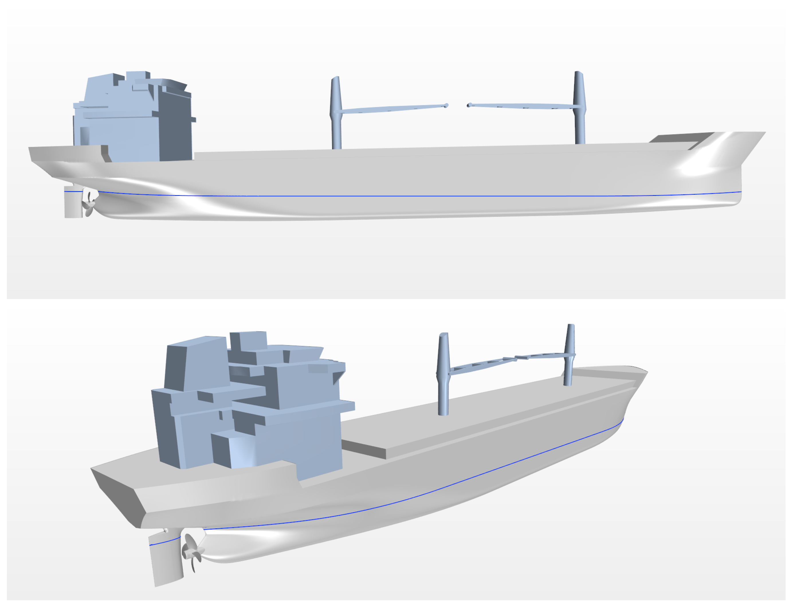
The open water simulations were performed in full-scale using the same propeller setup as in self-propulsion conditions. This means that, unlike a conventional open water model test setup, the propeller was not driven from downstream but from upstream. As a result, it operated in a pushing mode behind the ship hull, similar to the setup in propulsion conditions, and had the same hub cap. This setup is illustrated in
Figure 3, which also provides an overview of the overall mesh refinement pattern around the propeller.
The cylindrical rotating propeller region used in the sliding mesh calculation has the dimensions 0.125D (upstream), 0.288D (downstream), and 0.5385D (radius), measured from the propeller plane, where D represents the propeller diameter. These dimensions are smaller than those typically applied in the SINTEF Ocean standard open water CFD setup, because, in the self-propulsion case studied in this work, the propeller region had to be accommodated within a tight space between the ship hull and the rudder, as shown in
Figure 2. The rationale was then to use the same region dimensions in open water calculations to avoid the influence of region size when deriving propulsion factors. The respective dimensions of the main fluid region (also cylindrical in this case) were 5D (inlet), 15D (outlet), and 5D (radius), measured from the propeller centre. Additional simulations were performed to assess the influence of the downstream extension of the sliding mesh region on propeller open water characteristics and the quality of propeller slipstream resolution.
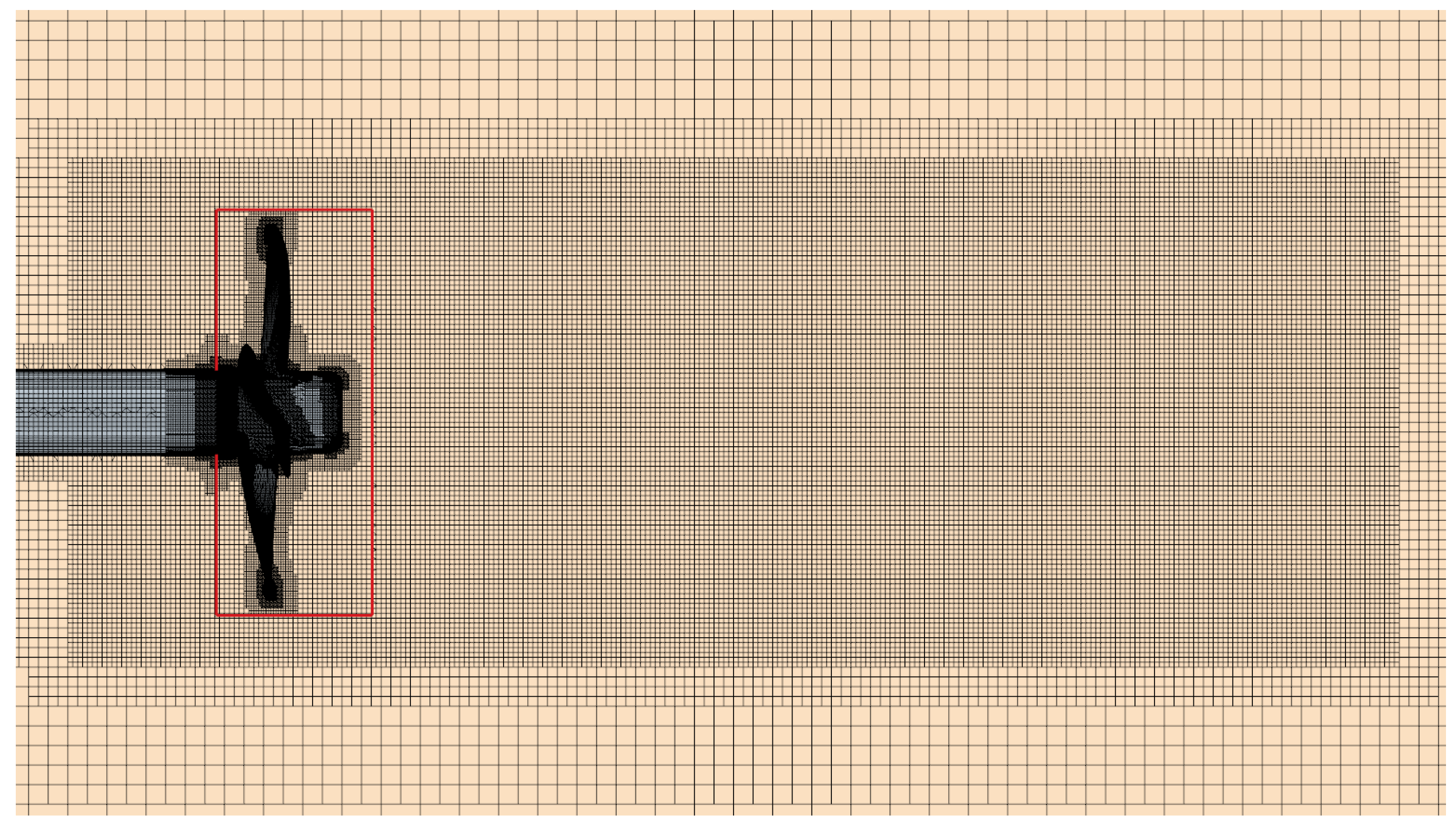
The cell size in the propeller region and the first (finest) volumetric control around the propeller and slipstream (as depicted in
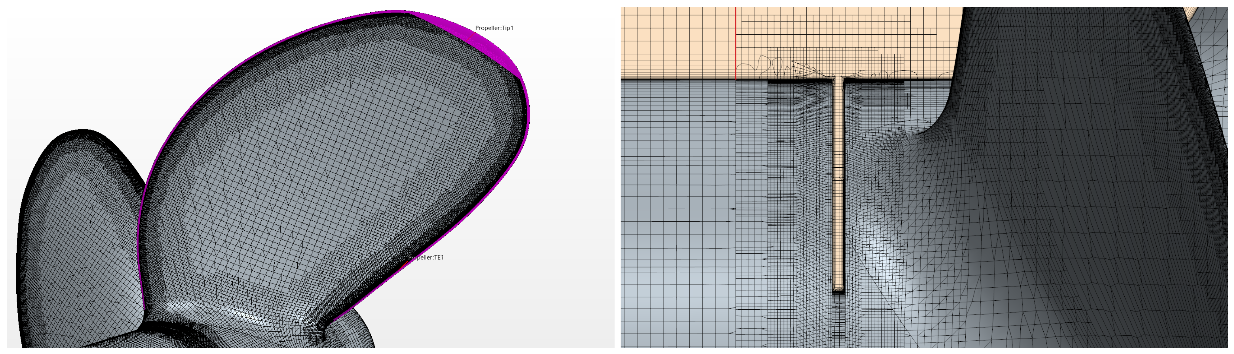
Figure 3) were set to 1.3% of the base size, which corresponds to the propeller diameter, D. The volumetric control extends to the distance of 3D downstream. On the propeller blades, the maximum target cell size is 0.65% of base, and it is reduced to the minimum size of 0.0203125% of base at the blade edges and tip. The edge and tip refinements are achieved using the surface patches extracted from the initial CAD geometry of the propeller, as shown in
Figure 4. In the absence of such patches, similar refinement can be achieved by means of volumetric controls in the shape of a tube following the leading edge feature curve, typically obtained from blade surface wireframe. The propeller model included a gap between the rotating propeller hub and the stationary shaft, measuring 17 mm in size, which is consistent with the self-propulsion setup. The inclusion of the hub gap in the numerical model allows for more accurate computation of forces acting on the propeller by avoiding uncertainty related to the integration of pressure on the side of the propeller hub facing the shaft. The total number of cells in the open water setup was 22.1 million, of which 18.6 million were accommodated in the propeller region.
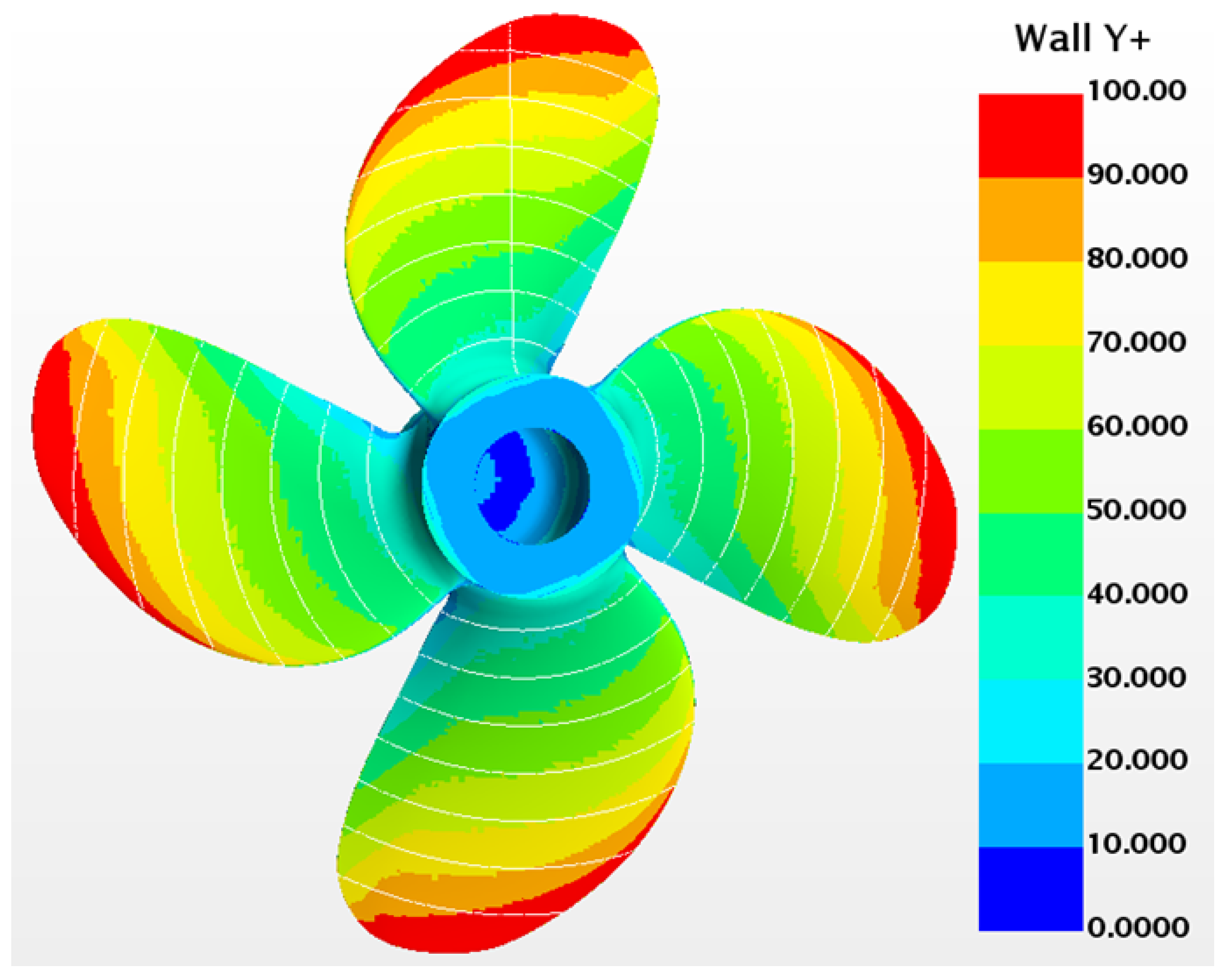
Figure 5 illustrates the arrangement of prism layers on propeller blades. The prism layer mesh consists of 10 layers. The height of the first near-wall cell is selected to target an average Wall Y+ approximately 60 in the middle section of the blade. This choice implies the use of wall functions, which offer computational efficiency and inclusion of surface roughness. The total thickness of prism layers is 0.235% of the propeller diameter. The present settings result in a layer stretch factor of approximately 1.35 and Wall Y+ distribution shown in
Figure 6. With a coarse near-wall mesh, one cannot achieve a uniform distribution of Y+ over the whole blade. However, as depicted in the figure, the applied settings provide a favourable Y+ range between 30 and 100, avoiding buffer zones everywhere except the gap and hub vortex separation area. The same Y+ range on the propeller is also met at other advance coefficients and in self-propulsion calculations.
In the open water scenario, several turbulence modelling approaches were investigated. These included (i) the traditional unsteady RANS method using the k-
SST model with linear constitutive relation [
23]; (ii) the Improved Delayed Detached Eddy Simulation (IDDES) method [
24], which incorporates a subgrid length-scale dependence on the wall distance. This allows the RANS part of the solution to be utilised in the thin near-wall region where the wall distance is smaller than the boundary layer thickness. The DES formulation with the k-
SST turbulence model in the RANS zones was employed [
25]; (iii) Large Eddy Simulation (LES) method with the Smagorinsky Subgrid Scale model [
26] and Modified Van Driest damping function [
27]; (iv) Scale-Resolving Hybrid (SRH) turbulence model [
28], which is a continuous hybrid RANS-LES technique. It switches continuously (unlike the DES method) from the RANS model to the LES model when the mesh resolution is fine and the time step is small. Similar to the DES solution, the SRH method was applied with the k-
SST model in the RANS part of the solution.
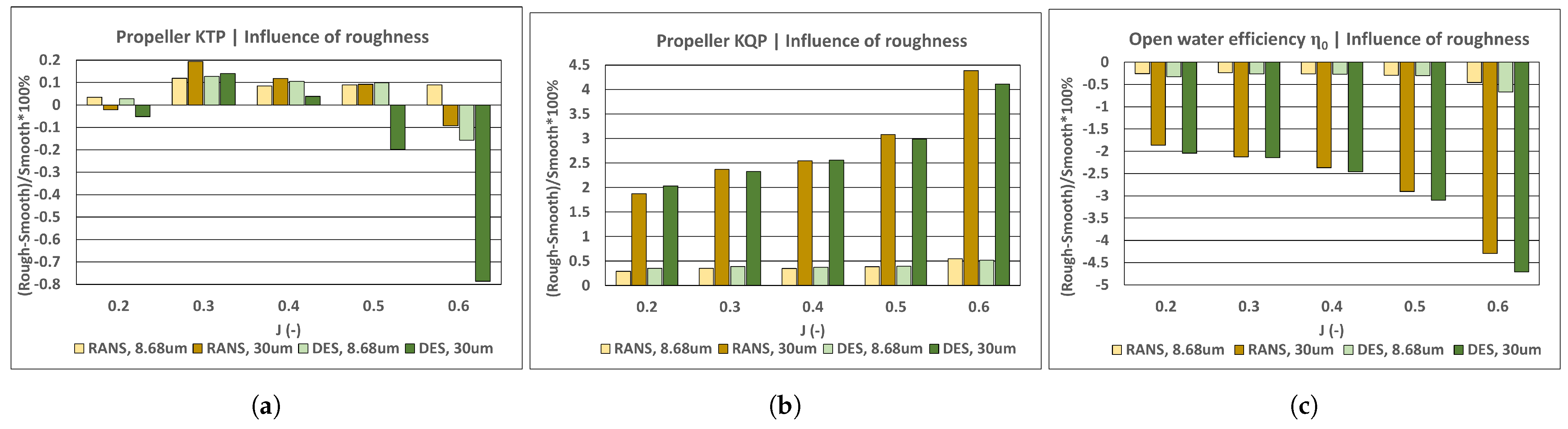
Open water calculations were performed with both smooth and rough propeller surfaces. The influence of surface roughness was accounted for by using roughness-modified wall functions, which shift the log layer of the inner part of the boundary layer closer to the wall. Mathematically, it is achieved by means of a roughness function [
29] that modifies the log law offset coefficient depending on the equivalent sand-grain roughness height, viscosity, and velocity scale. The influence of roughness was investigated only with the RANS and DES methods, considering the two values of roughness height: 8.68
m resulting from the JoRes propeller surface roughness measurements and 30.0
m, which is a standard value of sand-grain roughness used at SINTEF Ocean in CFD calculations on older ship propellers in service that have undergone cleaning and polishing before trials.
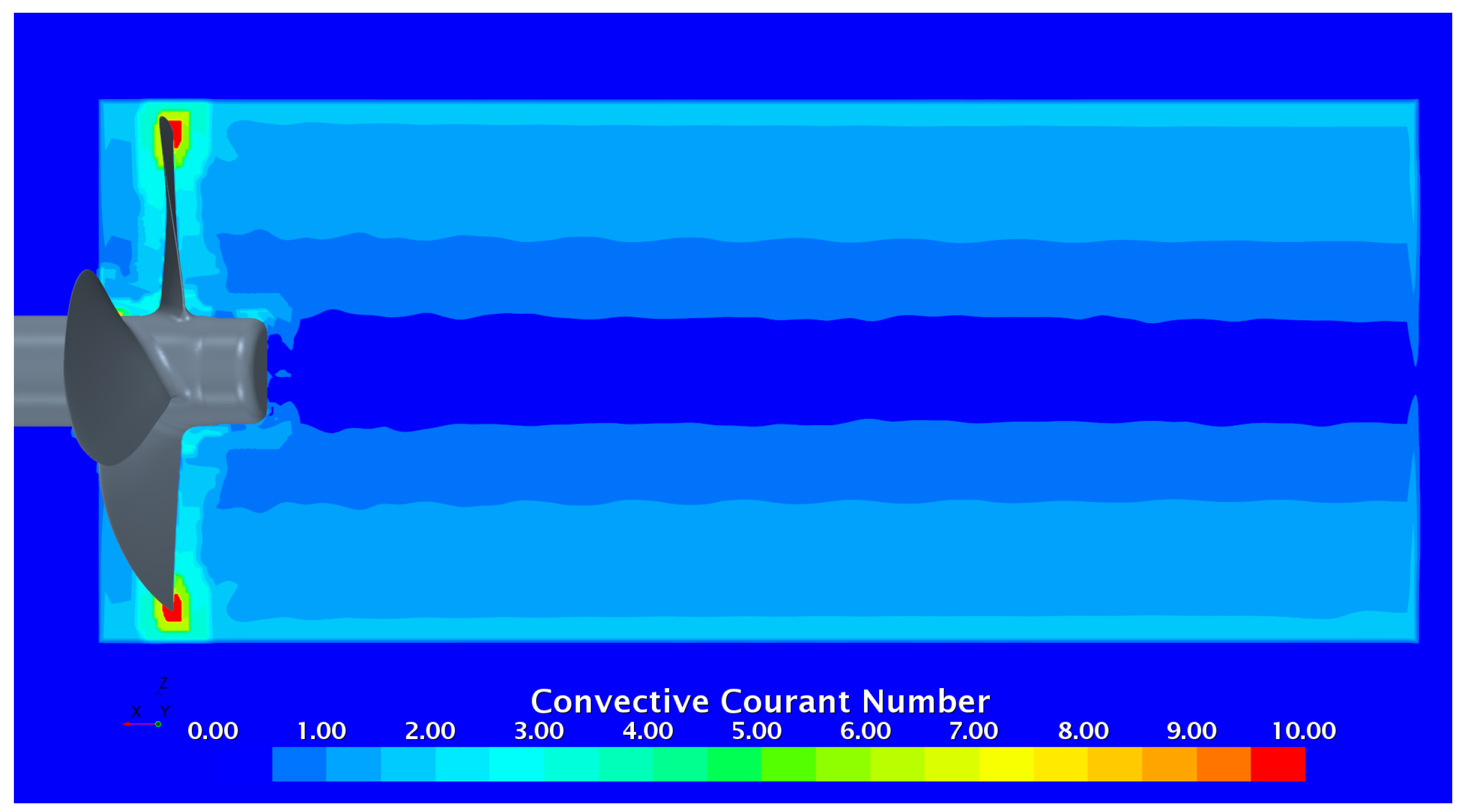
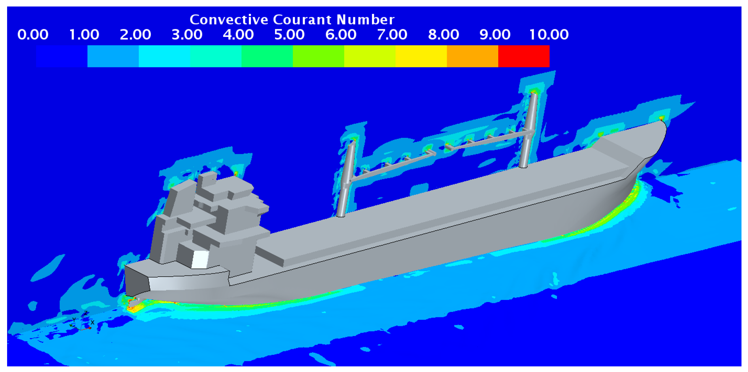
The time-accurate solution is achieved by rotating the sliding mesh region (propeller region) about the shaft axis with a specific angular step. The time step corresponding to 2 deg of propeller rotation was applied in both the open water and self-propulsion calculations, which in the authors’ experience is sufficient in most practical cases. However, an additional test with a step of 1 deg was conducted to assess the sensitivity of the LES and SRH models to time step size. Representative levels of Courant number obtained with the time step of 2 deg are shown in
Figure 7. Reducing the time step to 1 deg lowers the Courant number by a factor of 2.
The open water simulations were performed using the multi-phase flow formulation with the Volume of Fluid (VOF) model, as in the self-propulsion calculations, but with the reference pressure set to atmospheric conditions to prevent occurrence of cavitation.
3.2. Hull Resistance Simulations
The resistance simulations were performed in full scale using a geometry model consisting of the ship’s hull, rudder, and propeller hub. The calculation matrix included both cases with and without superstructure and cranes to evaluate their influence on the ship’s resistance and dynamic position. The initial hydrostatic position for the resistance simulations was the same as in the self-propulsion case, and it corresponded to the draught marks provided by JoRes as specified earlier.
The dimensions of the rectangular computation domain were assigned according to existing practises to minimise the influence of the outer boundaries on the quality of the numerical solution: 4LPP in X (inlet and outlet) and Y (side boundaries) directions from the ship’s aft perpendicular/centre plane, 2LPP in the Z direction to the bottom boundary, and 1LPP in the Z direction to the top boundary, from the base. As an additional measure to mitigate wave reflections, the VOF damping method described in [
30] was employed, with the damping zone extending to a distance of 2LPP from the inlet, outlet, and side boundaries. The resistance simulations were performed using the full hull model.
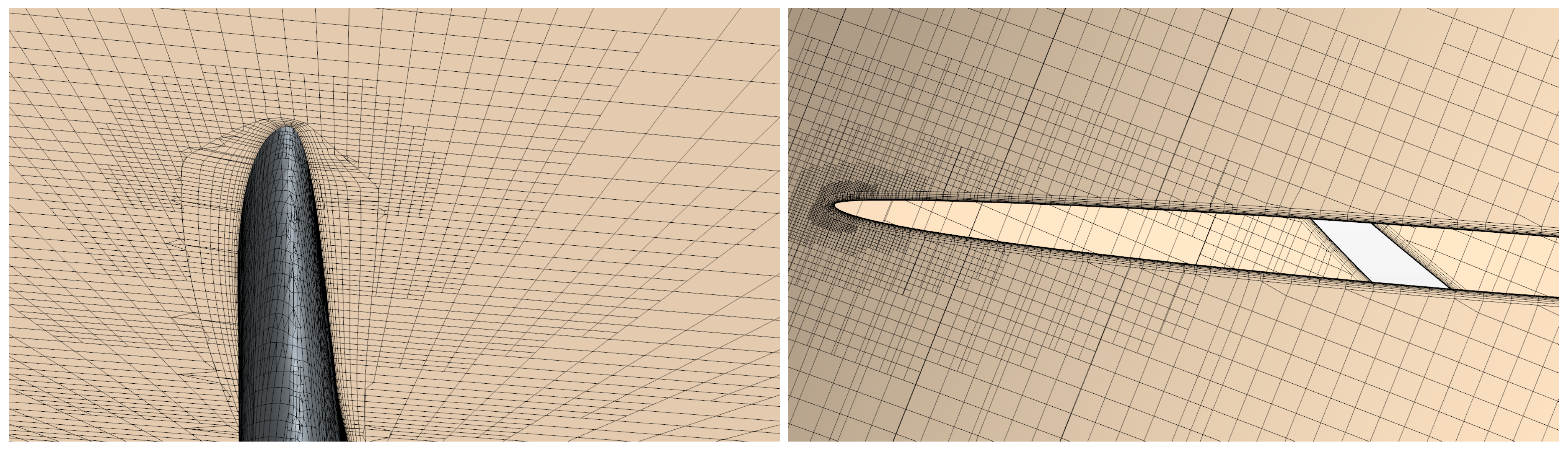
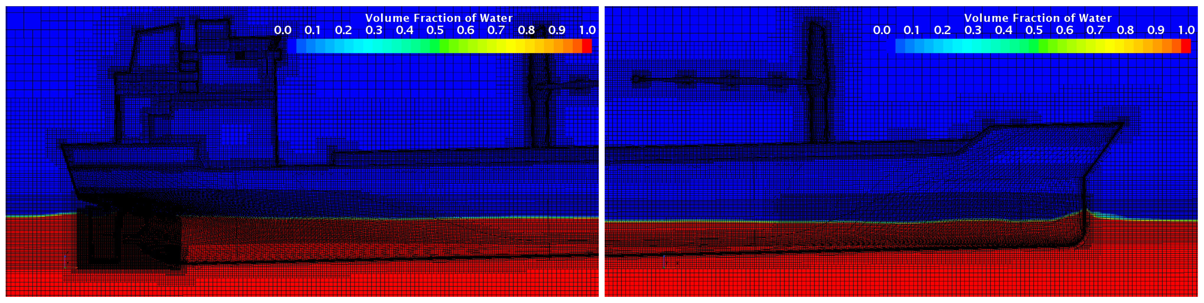
The Trimmer hexahedral mesh employed in the resistance case was designed to ensure refinement near the free surface, with a size equal to 0.1% of LPP in the Z direction. In the bow and stern regions, this size also applies to the isotropic cells around the hull. In the mid-ship area, the cells are anisotropic, with aspect ratios varying from 2 to 4. Conventional Kelvin’s wake refinement controls were used to capture the wave systems generated by the ship.
Figure 8 and
Figure 9 give illustrations of the mesh around the ship hull with superstructure and cranes, and in the area of free surface.
Additional mesh refinement controls are implemented around the propeller and rudder locations to ensure an adequate level of refinement for capturing the key characteristics of the separated hull wake. In this specific area, the refinement pattern is isotropic, and the cell size is set to 1.35% of the propeller diameter, which matches the size applied in the propeller slipstream in open water and self-propulsion calculations.
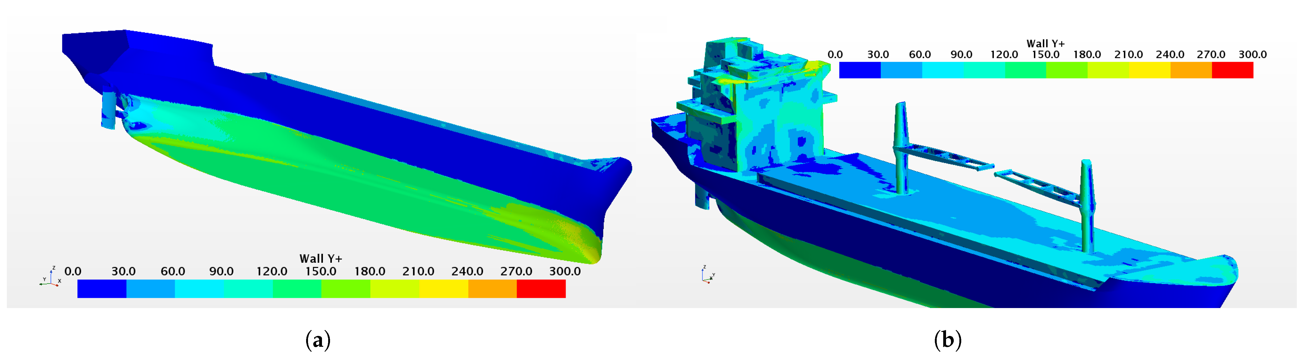
The prism layer mesh on the hull consists of 16 layers, with the height of the first near-wall cell chosen to target an average Wall Y+ of approximately 130 on the hull and 50 on the rudder. The total boundary layer thickness is chosen based on the consideration of stretch factor (which varies between 1.30 and 1.35) and reasonably smooth transition to the core mesh, which is particularly relevant in the stern area. A typical distribution of Wall Y+ on the ship is presented in
Figure 10a. As in the case of the propeller, it is impossible to provide a uniform distribution of Y+, but its values are kept above the buffer region (i.e., above 30) everywhere except in the flow separation zones.
The number of prism layers on the deck, superstructure, and cranes is reduced to 6. Because these parts are subject to intensive separation of the air flow with multiple stall areas, the Y+ varies significantly. However, the range of Y+ between 30 and 240 is well preserved, as shown in
Figure 10b. The total number of cells in the resistance setup is 15.8 million, which is higher than the usual count in routine resistance calculations. This is primarily due to the inclusion of on-deck features and the finer resolution of propulsor area.
The numerical solution for the free surface is obtained using the VOF method with the Flat VOF Wave model and the blended High-Resolution Interface Capturing (HRIC) scheme [
31]. The Courant number limits in the blended HRIC scheme are set to high values (Co
l = 200 and Co
u = 250) to ensure that the HRIC is used irrespective of the time step. These settings mitigate solution dependency on the chosen time step, which is essential when processing the results of resistance and self-propulsion calculations, such as deriving the thrust deduction factor. A representative distribution of Courant number around the ship observed in the resistance simulations is shown in
Figure 11.
The Courant number remains below 2.0 for the greatest part of the domain, but it increases to 7.0–8.0 in the regions where the ship’s bow and stern wave systems are generated and to 9.0–10.0 in the area where the stern wave interacts with the rudder. These higher values of Courant number are a natural consequence of the high induced velocities and finer mesh size in these specific areas. In propulsion simulations, due to the small time step (t∼2 deg), the Courant number remains well below 1.0 throughout the domain. Special tests were conducted to verify that the mentioned differences in Courant number have little, if any, impact on the computed ship resistance.
The Dynamic Fluid–Body Interaction (DFBI) model with two degrees of freedom in heave and pitch was used to solve the hydrodynamic position of the ship. The DFBI solver was applied to the whole domain. The equilibrium body motion option was chosen to accelerate convergence towards the sought-after steady-state solution. On the cautionary, it needs to be noted that, depending on the case, the equilibrium solution may lead to large variations in the body’s position at intermediate time steps and introduce disturbances that remain in the numerical solution for a long time. This effect is particularly noticeable in the DFBI solutions conducted without mesh morphing.
The turbulence model investigations primarily focused on two solutions: the RANS method with the k- SST model and the IDDES method with the k- SST model in the RANS domain. Preliminary studies on the case without superstructure also included the LES method, which was found to provide a good prognosis of total resistance of the smooth hull but had larger discrepancies with the RANS and DES solutions in terms of pressure and viscous resistance components. Furthermore, the LES model is not applicable with rough surfaces, which limits its use in the present case where the influence of hull roughness is essential. The results obtained with the SRH model revealed dependency on time step, because as the time step decreases, a larger part of the solution is treated by LES, and eventually when the time step is small (as in the self-propulsion case), the SRH solution is found to be equivalent to that of LES.
Assigning an appropriate value of sand-grain roughness to the ship’s hull required separate investigations. Initially, a surface roughness of 3.244 mm was provided in the JoRes case description from measurements on the hull using an underwater roughness scanner. Such a high reported value of average hull roughness may be caused by the following main factors: vessel age, quality of underwater hull cleaning, and method used for conversion of locally measured values. Furthermore, the available photos of the hull surface revealed numerous patches, pits, and bumps, which can be considered macro-scale roughness measured in millimeters rather than micrometers. At a later stage, JoRes provided another estimation of hull roughness using an alternative approach, resulting in a value of 440 m. Converting the measured value of technical averaged hull roughness (AHR) to the equivalent sand-grain roughness height used in the wall functions is not a straightforward process. Therefore, the value of this parameter was derived from additional calculations with a flat plate model.
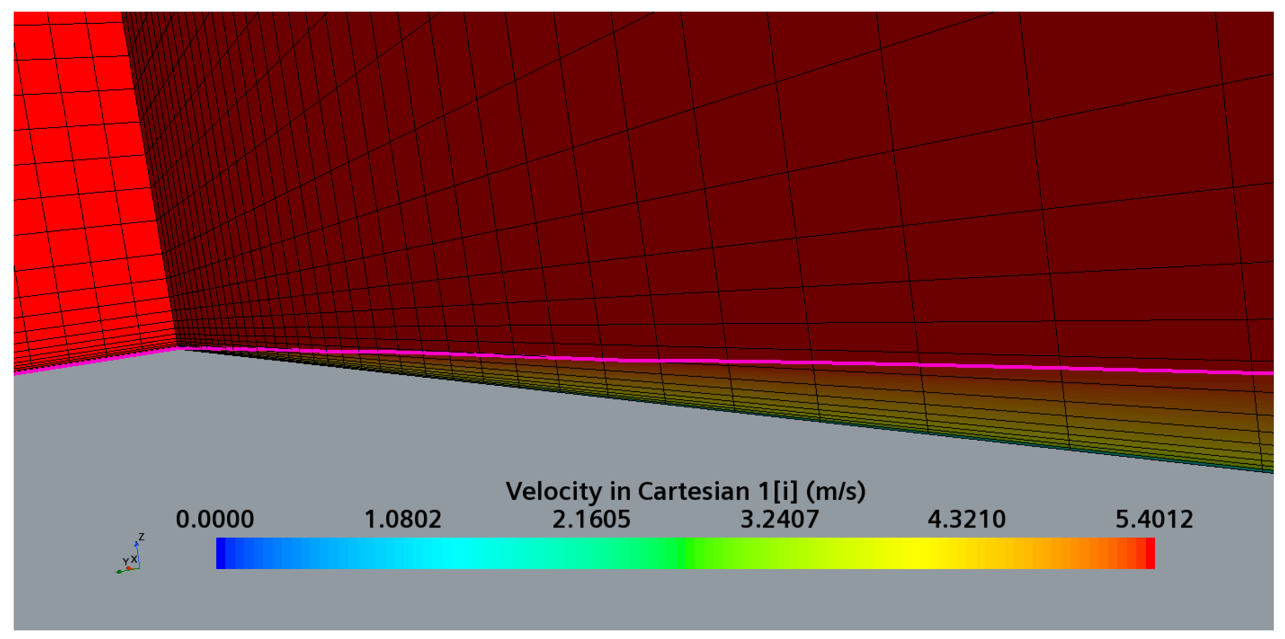
In these calculations, the computational domain consisted of a rectangular box of length equal to the ship’s LPP. The bottom surface of the domain was set as the no-slip wall boundary, representing the flat plate. The upstream boundary was designated as the velocity inlet, while the downstream and top boundaries were set as pressure outlets. The side boundaries were imposed with a symmetry boundary condition. The computation mesh was constructed to replicate the prism layer mesh settings used in the ship resistance calculations and provided the same target Wall Y+. At the inlet, a Blasius velocity profile was utilized, which represents the theoretical solution for the streamwise and normal velocities in the laminar boundary layer over a smooth plate. This was done following the recommendation from the JoRes case description [
20] in an attempt to mitigate a slight acceleration in the boundary layer that may occur locally when using a constant velocity profile. The Blasius profile applied at the inlet was calculated at a distance of x/L = 0.005 from the plate leading edge. A comparison between the two methods to set up the inlet velocity revealed that local flow acceleration downstream of the inlet is reduced and the displacement velocity decreases somewhat faster along the plate when the Blasius profile is applied. However, only very minor differences between the two solutions were found in the computed distributions of the local friction coefficient and in its integral value. The calculations were performed with a smooth surface and an equivalent roughness height (r
g) of 50, 100, 15, and 200
m.
Figure 12 illustrates the computation mesh and the field of streamwise (axial) velocity in the near-wall region of the smooth flat plate.
In
Table 2, the computed values of the integral friction coefficient (C
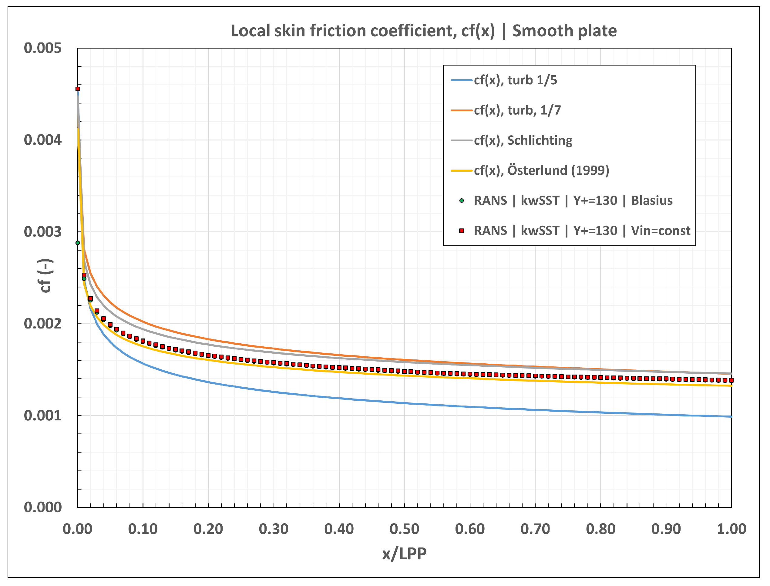
F) are compared with the ITTC friction lines used in ship performance prediction procedures and the experimental correlations by Österlund [
32]. The calculation results for the smooth plate are approximately 2% below the ITTC57 friction line [
33] and 1% above the experimental results by Österlund. The computed streamwise distributions of the local friction coefficient (cf) are presented in
Figure 13, where they are compared with different theoretical solutions and experimental correlations. The results show good agreement with Österlund’s data.
Regarding the case of a plate with roughness, the ITTC57 friction line results for C
F corrected with the ITTC78 roughness allowance according to Townsin [
34,
35] are found to be between the CFD results for the flat plate with sand-grain roughness heights of 50
m and 100
m, as shown in
Table 2. Based on these findings, a sand roughness height of 80
m was chosen to be applied in the main resistance and self-propulsion simulations for comparison with the predictions based on model test data. To assess the influence of higher roughness, and considering the high roughness values measured on MV REGAL, additional simulations were performed with r
g = 150
m. The same values of roughness height were applied to the ship’s hull and rudder surfaces.
3.3. Self-Propulsion Simulations
As for the topology of the computation domain, mesh regions, and mesh settings on the ship and propeller, the self-propulsion simulation setup is largely a combination of the setups used in the resistance and open water simulations.
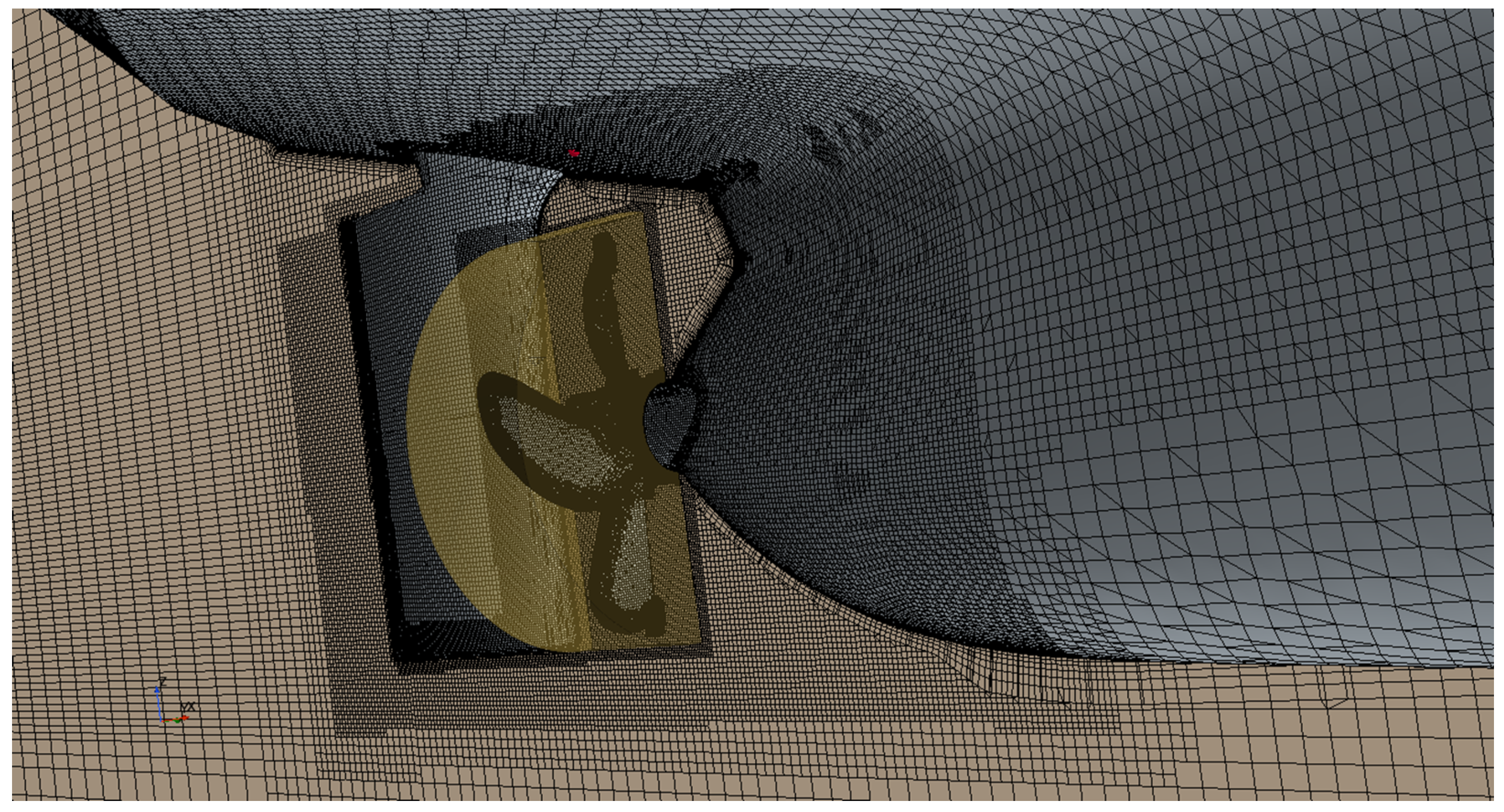
Figure 14 provides an illustration of the mesh in the aftship area, where the sliding mesh propeller region is fitted between the ship hull and the rudder. Similar to the open water case, this region accommodates the entire propeller hub and cap. The total number of cells in the self-propulsion setup is 32.8 million, with 13.3 million cells in the main fluid region and 19.5 million cells in the propeller region.
The self-propulsion calculation is performed in several steps. In the first step, the propeller region is fixed, and the solution is performed using the Moving Reference Frame (MRF) method until convergence is attained for the free surface flow. In the second step, the sliding mesh region is set in motion with the initial value of propeller RPM. The RPM is subsequently adjusted to determine the vessel’s self-propulsion point, where the force balance Equation (
1) is satisfied:
where
is the ship resistance with an operating propeller,
is the correction accounting for additional resistance components that are not modelled in the simulation (set to 0 in the present case),
is the X-component of propeller thrust, and
is the solution tolerance (set to 0.5% of propeller thrust).
Finally, in the third step, the phase transfer solver with the cavitation model by Scherr-Sauer [
36] is activated. The saturation pressure is gradually ramped through the first propeller revolution to its value specified in water properties to address the possible occurrence of cavitation. During the cavitation calculation, it is assumed that thrust-resistance balance is not violated, and therefore propeller RPM is fixed to its value determined in the second step.
In the present study, the ship’s position was fixed in the self-propulsion analysis using the dynamic sinkage and trim values obtained from the DFBI resistance calculation. Both RANS and DES turbulence modeling approaches were investigated, with an equivalent sand grain roughness height of 80 m applied to the ship hull and rudder, and a roughness height of 30 m to the propeller. An additional run with the RANS method using a roughness height of 150 m on the hull and rudder was conducted after the fashion of resistance analyses.


 and
and 


