Numerical Modeling of Nearshore Wave Transformation and Breaking Processes in the Yellow River Delta with FUNWAVE-TVD Wave Model

Abstract

The presence of wave coherence, which contributes to the inhomogeneity of wave characteristics and significantly affects wave processes over nearshore regions of the Yellow River Delta (YRD), was simulated and analyzed in this study. A phase-resolving Boussinesq-type wave model, FUNWAVE-TVD, was used to simulate waves with desirable coherency effects. Bathymetry and topography data were obtained from the Chinese nautical chart and E.U. Copernicus Marine Service Information. After the model configuration, spatial distributions of the root mean square and significant wave heights, and the maximum cross-shore current velocity and vorticity over the domain with respect to different degrees of wave coherence and energy spectrum discretization were investigated. The results indicate that the complexity of the spatial distribution and magnitude of longshore variations in wave statistics are proportional to the degree of coherence. Waves with higher coherency exhibit more complex variabilities and stronger fluctuations along the longshore direction. The influence of morphological changes on wave height in the YRD was discernible by comparing the results with and without coherency effects. The cross-shore current velocity decreased as the waves moved toward the surf zone, while the vorticity accelerated, indicating a higher shear wave magnitude. The simulated wave dissipates more than 60% (80%) of its energy when it reaches water depths of less than 5 m (2 m) and completely dissipates when it breaks at the shore.

1. Introduction

Coastal regions range from estuaries and shallow coastal areas to shelf breaks [1], which provide important natural resources that are fundamental for the present and future generations of coastal communities [2]. However, the coastal environment has been facing enormous pressure, including rapid changes in the global climate and the influence of human activities, which leads to significant risks and hazards in coastal erosion [3], tidal flooding [4], and changes in coastal morphology [5]. Complex hydrodynamics in nearshore regions have drawn great attention in the past half-century. With the development of computational power and numerical methods in the past two decades, the modeling of physical processes in coastal domains has achieved significant advances in various fields by using unstructured grids, model nesting techniques, data assimilation, and model coupling. Many studies on the application of numerical models have helped researchers solve complex problems that cannot be handled by physical models (or are too expensive to compute), overcome the lack of field observations and measurements, and provide valuable hydrodynamic simulations in coastal regions. Consequently, coastal modeling has become an important and effective tool for achieving remarkable results.

However, recent numerical models have certain limitations. Recent findings indicate that coastal researchers have focused on model coupling, data assimilation, nearshore processes, cyberinfrastructure, model skill assessment, observing system design and operation, probabilistic prediction methods, and early prediction. In terms of nearshore wave dynamics, many studies have been conducted to investigate critical factors that affect wave transformation and breaking processes, such as wind–wave interactions [6,7], wave–current dynamics [8,9], breaking wave-induced dissipation [10,11], transient wave and reflection [12,13,14], wave run-up, and rip currents [15,16,17,18]. Despite recent advances in numerical modeling, these models have major limitations. One of the ad hoc aspects of model development is the treatment of coherency effects. Accurate simulations of nearshore waves are critically dependent on accurate modeling of the impacts of coherent waves on the interference patterns of wave characteristics (e.g., mean surface elevation, wave height, current velocity, and vorticity).

Wave coherence is a significant phenomenon that occurs when a pair of individual waves with identical frequencies and constant phase differences interact with each other and form a stationary interference in the wave field. For the water waves, coherent waves affect wave processes in coastal regions, which leads to spatial inhomogeneity in the wave characteristics [7,19]. Wave coherence potentially affects the longshore distribution of wave statistics, including wave heights [20,21,22], wave-induced nearshore circulation and rip currents [18,23,24], vorticity, and wave breaking [25,26]. Because previous modeling studies were mainly based on ideal experiments, they could not fully evaluate practical issues with realistic bathymetries and topographies [27]. Therefore, this study aimed to enhance the understanding of nearshore wave transformation and breaking processes influenced by primary parameters (e.g., varying bathymetry, energy spectra, and wave coherence) in a realistic domain.

Albeit important, it is relatively challenging to simulate coherent interference at the field scale. Among the early works on wave coherence modelling, phase-averaged models based on the radiative transfer equation (RTE) have frequently been applied to replicate the impacts of coherent interference in the wavefield. The RTE-based model assumes that the wave field remains quasi-homogeneous and near-Gaussian and that the wave variance density transfers through a slowly varying medium (e.g., currents and topography). They require boundary conditions that are mainly satisfied in the open ocean and restrict the model capability in resolving inhomogeneous patterns caused by coherent waves in coastal regions [28]. Considerable efforts have been made to alleviate this limitation through the continuing development of a third-generation phase-averaged wave model [29], with newly proposed transport equations incorporating coherency effects [28,30], a source term dealing with depth-induced wave breaking [31], a bi-spectral evolution equation handling non-Gaussian wave characteristics in shallow water regions [32], and recent improvements in wave–current interaction [33].

Owing to the explicit retention of phase information, phase-resolving Boussinesq-type [34,35,36,37] and nonhydrostatic models [38,39,40] provide alternative approaches for the direct modeling of wave interference patterns prompted by coherent waves, wave–wave interaction, and breaking-induced nearshore circulation. FUNWAVE-TVD was fundamentally developed with parallel computing and adaptive mesh refinement (AMR) in modelling waves at either the coastal or basin scale, and its computational time was less than that of nonhydrostatic models. Owing to the wave energy discretization techniques of the source function [41], coherent waves in the Boussinesq-type model are synergistically generated by the topographic characteristics of the domain and numerical wavemaker from the offshore boundary. The latter source makes it more challenging to separate the impacts of the coherency effects and longshore variations induced by bathymetries in coastal waves, as the default wavemaker of the FUNWAVE-TVD model could generate artificial longshore variations of nearshore processes. Numerous efforts have been devoted to avoiding ambiguity in this problem, such as increasing the discretization in both wave direction and frequency [42] or the proposed method for the discretization of the input spectrum [17,43]. Furthermore, Salatin et al. [44] proposed a new wavemaker, which is a generalized form of the default wavemaker in the FUNWAVE-TVD model that can eliminate and control the degree of wave coherence [44].

The objective of the present study is to further investigate the impacts of five levels of wave coherence, associated with different input energy spectra, on the spatiotemporal distribution of wave statistics in the nearshore area of the Yellow River (Huanghe) Delta (YRD), China. Because of the high computational cost of a phase-resolving model [45], studies on this relatively large-scale area are limited. For accurate model simulations, this study introduced a flexible approach to derive high-resolution bathymetries for the domain of interest. The YRD is located between Bohai and Laizhou Bays in the semi-enclosed Bohai Sea. Many studies on wave dynamics have been conducted in the Bohai Sea, such as the assessment of wave energy [46], wave generation and dissipation during cold-wave events [47], and storm surge variations along the coastline [48]. However, there are limited studies on the numerical modeling of coastal hydrodynamics and wave–current interactions over the nearshore of the YRD. While most recent studies have focused on applying remote sensing and geographic information system (GIS) tools to assess coastal risks and vulnerability, in the case of the modeling approach, most studies have only focused on the simulation of tidal levels and currents [49] or applied the hydrostatic model to solve RANS equations [50]. Few comparative studies have focused on the impact of wave coherence on the spatial variability of wave processes in the nearshore region of the YRD. Moreover, previous studies have rarely used the latest coastline in their models. Although high-resolution bathymetries and accurate coastlines are significant in nearshore modeling, they are overly expensive to obtain using conventional field survey techniques such as echo-sounding and LiDAR (e.g., airborne light detection and ranging) measurements. The present work uses interpolated high-resolution bathymetric data extracted from a nautical chart, and this proposed approach can be applied to simulate wave processes over the nearshore of other delta regions.

In short, the key questions for advancing the understanding of nearshore wave processes in the Yellow River Delta are: (1) How do different levels of wave coherence affect the spatial distribution of wave field in the nearshore region, and (2) How does the morphological change affect the wave transformation and breaking processes with and without coherency effects? The present study addressed these questions by employing FUNWAVE-TVD, a phase-resolving Boussinesq-type wave model, to simulate the wave transformation and breaking processes in the nearshore region of the Yellow River Delta, with a focus on the impact of wave coherence. In the next section, the study area and detailed procedure for generating proper bathymetric data are described, followed by a brief introduction of the FUNWAVE-TVD model, newly proposed wavemaker, model configuration, and skill assessment of depth model. The impacts of different degrees of wave coherence and input energy spectra on the spatiotemporal variabilities of wave statistics (e.g., root mean square and significant wave height, maximum cross-shore current velocity, and vorticity) over the YRD are analyzed and discussed in Section 3. Finally, the conclusions are presented in Section 4.

2. Methodology

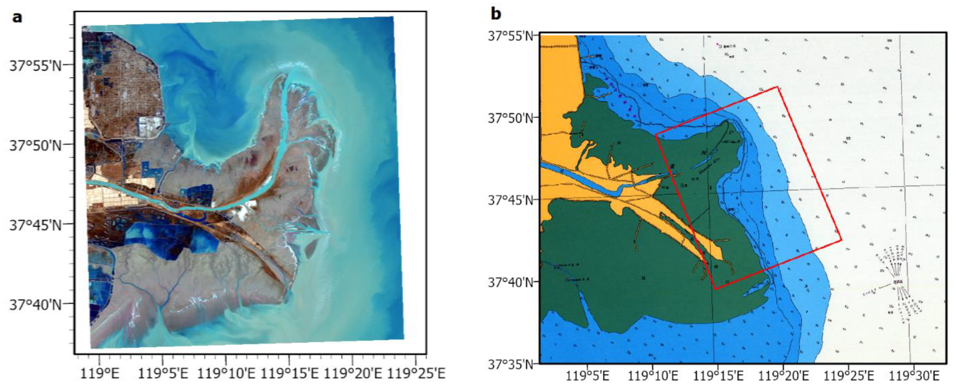
2.1. Study Area and Data Sources

The Yellow River Delta (YRD) lies in the interior of the semi-enclosed Bohai Sea, north of Bohai Bay, and east of Laizhou Bay (Figure 1). The entire drainage basin of the Yellow River covers an area of approximately 750,000 km² and its carried sediments have formed the YRD since 1855 [51]. The modern YRD, located in the northeast of Dongying City, Shandong Province, includes five counties (i.e., Dongying, Hekou, Guangrao, Lijin, and Kenli) and covers approximately 5500 km² land area between the Bohai and Laizhou Bays. Laizhou Bay is south of the Bohai Sea and stretches from the modern YRD (37.8° N, 119.1° E) in the west to Qimu Island (37.67° N, 120.65° E). The bay is bowl-shaped, with an average (maximum) water depth of <10 m (18 m). Its surface area is ~7000 km², with an ~300 km coastline [52].

To validate the performance of the wavemaker, this study used observation wave data collected every 30 min 17–23 May 2022 at ($37°{41}^{\prime }{56.4}^{″} \mathrm{N}$, $119°{21}^{\prime }{32.4}^{″}\mathrm{E}$) using BL900MM (Figure 2a). According to the data, the significant (root mean square) wave height in the offshore ranges from 0.14 to 0.76 (0.13 to 0.44) m, with a mean of 0.36 (0.23) m. In addition, the peak wave period ranges from 1.4 to 20.8 s, with an average of 3.3 s, and the mean wave direction is $145°$.

To obtain the bathymetric map, the depth values were digitized from the latest version of the Chinese nautical chart issued in 2011 and then used to construct a triangular irregular network (TIN), a vector-based digital geographic dataset representing the depth morphology. A 50 m resolution bathymetric map was created by converting the above TIN dataset to a raster file using the interpolation function of the ArcGIS application. In addition, this study employed ship-based multibeam gridded bathymetry data from the Global Multi-Resolution Topography (GMRT) database for validation. A thorough search of relevant databases revealed that the current version (GMRT v4.0, released in January 2022) provides the highest resolution (approximately 50 m grid size) among other public sources, such as GEBCO (15 arcsec grid) and ETOPO1 (1 arcmin grid). The GMRT data were downloaded on 3 March 2022 and georeferenced to the WGS 1984 datum, UTM projection Zone 50 N. Subsequently, depth data, either derived from the Chinese nautical chart or downloaded from the GMRT source, were mosaiced with Copernicus DEM gridded data (GLO-30) that covered the modern topography of the YRD to form a united bathymetric map. GLO-30 is a 30 m resolution cell-centered grid dataset with geographic coordinates that can be exported from the SNAP application.

To determine the appropriate resolution for model simulation, the mosaiced bathymetric maps described above were interpolated to exact grid sizes of 50, 10, 5, and 2 m using the cubic convolution resampling raster function in ArcGIS. Generally, resampling methods are applied to transform raster images of different resolutions into a uniform cell size and coordinate system. For data analysis, these resampled bathymetric maps are hereafter denoted with an ID, in which the letter part (NC and GMRT) refers to the data obtained from Chinese nautical charts and the GMRT database, respectively; the numbers (50, 10, 5, and 2) indicate the grid size in meters of the corresponding map.

2.2. Numerical Model

FUNWAVE-TVD is a recently developed total variation diminishing (TVD) version [34] of a widely accepted time-dependent phase-resolving wave-current model that was developed based on the fundamental theory of fully nonlinear Boussinesq equation [53,54] and its extensions [55]. The generalized conservative form of the Boussinesq equations is given by:

$$\frac{\partial \mathsf{\Psi }}{\partial t}+\nabla \cdot \mathsf{\Theta }\left(\mathsf{\Psi }\right)=S$$

(1)

where $\mathsf{\Psi }$ and $\mathsf{\Theta }\left(\mathsf{\Psi }\right)$ are the vector of conserved variables and the flux vector function, respectively, given by:

$$\begin{array}{c}\mathsf{\Psi }=\left(\begin{array}{c}H\\ U\\ V\end{array}\right),\\ \mathsf{\Theta }=\left(\begin{array}{c}{S}_{p}Pi+Qj\\ \left[\frac{S_p{P}^2}{H}+\frac{1}{2}{S}_{p}g\left({\eta }^2+2\eta h\right)\right]i+\frac{PQ}{H}j\\ \frac{S_{p}PQ}{H}i+\left[\frac{Q^2}{H}+\frac{1}{2}g\left({\eta }^2+2\eta h\right)\right]j\end{array}\right),\end{array}$$

(2)

where $\left(P, Q\right)$ is the horizontal volume flux, $\left(U,V\right)$ is the velocity component, and $H=h+\eta$ with h being the water depth and η being the surface elevation. $S$ represents the source term added to the governing equation [41,56], and $t$ denotes the partial differentiation with respect to time. S_p is the spherical coordinate correction factor defined for the spherical mode of FUNWAVE-TVD model; (i, j) is the location of a grid point in $x$ and $y$ direction in a Cartesian coordinate system; $g$ is acceleration constant due to gravity.

For spatial discretization, the FUNWAVE-TVD model employs a combination of finite volume and finite difference approaches to compute values and numerical fluxes at cell interfaces by applying a reconstruction technique and a local Riemann solver [57]. Both the low- and high-order MUSCL-TVD (Monotone Upstream-centered Scheme for Conservation Laws-TVD) schemes are implemented for the flux and first-order derivative terms. However, the modified fourth order MUSCL-TVD scheme [58] developed in the present version (v.3.6) was adopted for the high-order scheme to avoid numerical instability in long-term simulations.

For temporal discretization, a third-order strong stability preserving (SSP) Kutta scheme for nonlinear spatial discretization was adopted [59], which is written as

$$\begin{array}{c}{\mathsf{\Psi }}^{\left(1\right)}={\mathsf{\Psi }}^n+\mathsf{\Delta }t\left(-\nabla \cdot \mathsf{\Theta }\left({\mathsf{\Psi }}^n\right)+S^{\left(1\right)}\right),\\ {\mathsf{\Psi }}^{\left(2\right)}=\frac{3}{4}{\mathsf{\Psi }}^n+\frac{1}{4}\left[{\mathsf{\Psi }}^{\left(1\right)}+\mathsf{\Delta }t\left(-\nabla \cdot \mathsf{\Theta }\left({\mathsf{\Psi }}^{\left(1\right)}\right)+S^{\left(2\right)}\right)\right],\\ {\mathsf{\Psi }}^{\left(n+1\right)}=\frac{1}{3}{\mathsf{\Psi }}^n+\frac{2}{3}\left[{\mathsf{\Psi }}^{\left(2\right)}+\mathsf{\Delta }t\left(-\nabla \cdot \mathsf{\Theta }\left({\mathsf{\Psi }}^{\left(2\right)}\right)+S^{\left(n+1\right)}\right)\right],\end{array}$$

(3)

where ${\mathsf{\Psi }}^n$ denotes the $\mathsf{\Psi }$ at time level $n$, ${\mathsf{\Psi }}^{\left(1\right)}$ and ${\mathsf{\Psi }}^{\left(2\right)}$ are values at the intermediate stages in the Runge–Kutta integration. $S$ should be updated using (u, v, η) at the corresponding time step, and iterations are required to achieve convergence [60]. In addition, an adaptive time step is selected following the Courant–Friedrichs–Lewy (CFL) criterion, which is given as

$$\mathsf{\Delta }t=C_{CFL}min\left(\begin{array}{c}min\left[\frac{\mathsf{\Delta }x}{\left|u_{i,j}\right|+\sqrt{g\left(h_{i,j}+{\eta }_{i,j}\right)}}\right],\\ min\left[\frac{\mathsf{\Delta }y}{\left|v_{i,j}\right|+\sqrt{g\left(h_{i,j}+{\eta }_{i,j}\right)}}\right]\end{array}\right),$$

(4)

where $C_{CFL}$ is the Courant number; $\mathsf{\Delta }x$ and $\mathsf{\Delta }y$ are the grid sizes in the x- and y-axis directions, respectively; $g$ is the acceleration due to gravity; and $u_{i,j}$, $v_{i,j}$, $h_{i,j}$, and ${\eta }_{i,j}$ are the x- and y-axis velocities, local still water depth, and surface elevation at the grid point (i, j), respectively.

2.2.1. Wave Generation

The FUNWAVE-TVD model employs an internal wavemaker [41,56] to generate monochromatic or directional spectral waves by adding a straight longshore line with a nondimensional cross-shore width close to the offshore boundary of the computational domain. Internal wavemaker introduces a source function into the continuity equation to generate both regular and irregular waves corresponding to a given frequency and directional spectrum. Regarding the formulation of the wavemaker, this study adopted the newly proposed wavemaker developed by Salatin et al. [44], which considers the degrees of wave coherence. The wave energy spectrum of the FUNWAVE-TVD model was discretized in both frequency and direction. Each frequency bin accommodates several coherent wave components, resulting in artificial longshore variations in the nearshore processes. By applying a new single-summation method, the proposed wavemaker discretizes the input energy spectrum into finer frequency components. Each frequency corresponds to a single directional bin, resulting in no coherent waves generated in the wavefield and ensuring that the highest energy is associated with the mean direction and peak frequency. Therefore, an irregular wave field can be generated by the new wavemaker by superimposing the single-wave components. In addition, the new wavemaker can introduce a controllable number of coherent waves into the offshore boundary condition by defining a percentage of the generated waves, which is hereafter referred to as the degree of wave coherence. It can be displaced from the original to other frequencies, forming groups of coherent waves in the model domain for the desired purposes. This recent development of wavemaker formulation enables modelers to investigate the impact of wave coherence on hydrodynamic processes with respect to different coherent levels. Detailed formulae and descriptions of the newly proposed wavemaker and its components can be found in Salatin et al. [44].

2.2.2. Wave-Breaking Treatment

Two wave-breaking algorithms were employed in the FUNWAVE-TVD model. The first method implements conventional eddy viscosity using the TVD scheme. The second technique, based on the work of Tonelli and Petti [61], converts the Boussinesq equations into a nonlinear shallow water equation (NSWE) in cells, where the Froude number exceeds a predetermined threshold. This was achieved by disregarding the required dispersive terms and taking advantage of the shock-capturing mechanism with the TVD scheme. For model validation, numerical tests that replicated Mase and Kirby’s experiment [62] were conducted to evaluate the impact of different SWE criteria on the simulation of irregular wave breaking in shallow water.

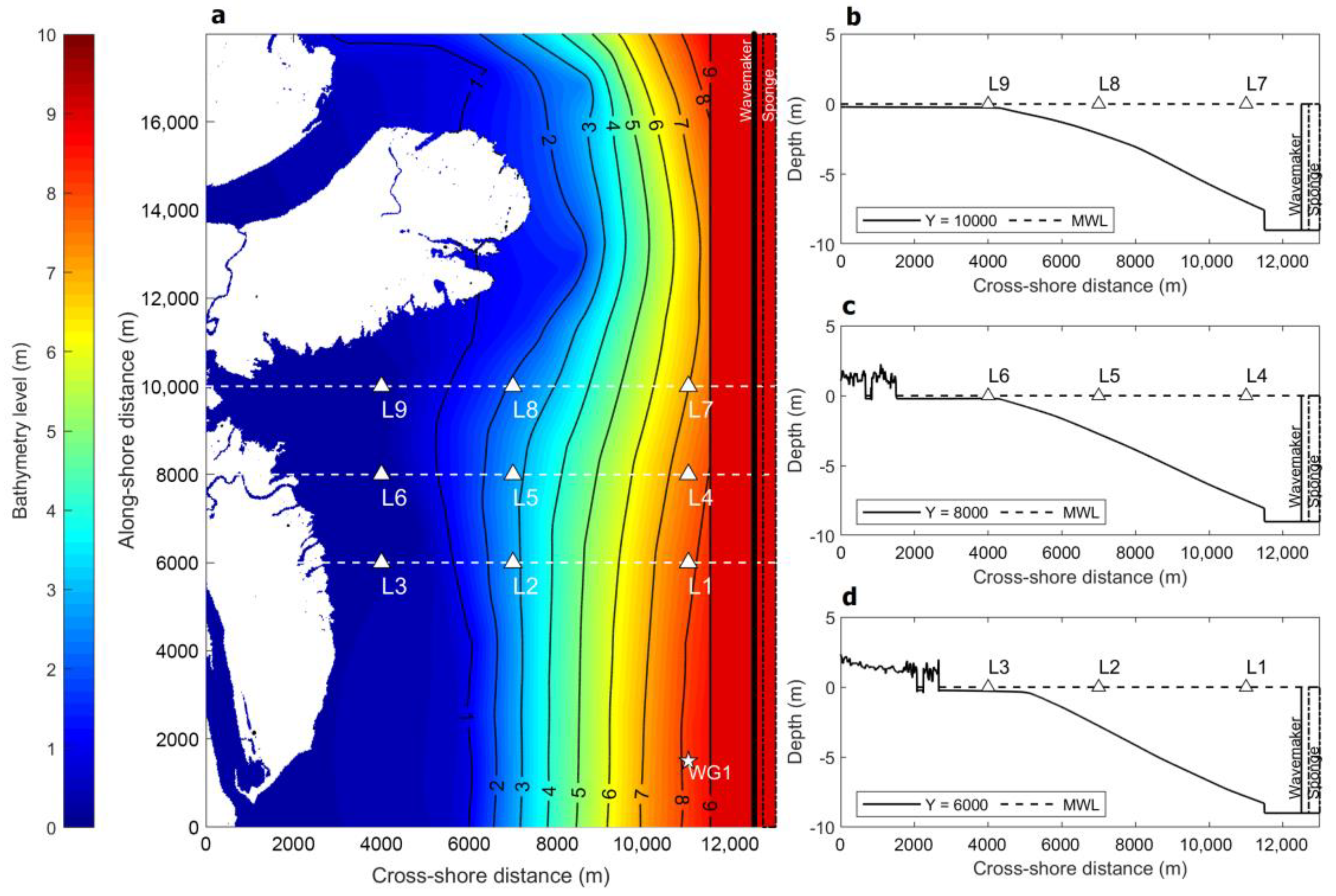
2.2.3. Model Configuration

To investigate the role of the offshore boundary conditions, idealized experiments were set up using the bathymetry data mainly derived from the nautical chart in the YRD and the initial wave conditions were employed from the wave characteristics measured by the wave buoy BL900MM located offshore of the YRD (Figure 2a).

The computational domain for the model configuration was defined based on the interpolated bathymetric map NC5 and covered ~18 and 13 km in the north-south and east-west directions, respectively, in Cartesian coordinates. The spatial resolution was 5 m in both directions, resulting in a matrix of 2600 × 3600 grid points in the x and y directions. The computational domain coordinates were rotated 21° clockwise from north. The model domain was expanded along the longshore direction to implement a periodic lateral boundary condition to generate an unrestricted longshore flow. In addition, wave reflection was fully reflected. To generate proper wave forcing [63], a 1500 m width flattened area with a constant depth of 9 m was created around the wavemaker, which was 500 m from the offshore boundary. To reduce the unintended reflection effects, a 300 m width sponge layer was applied. The total simulation time was 2 h with a time step of 1 s, resulting in a computation time of approximately 12 h to derive the selected model output, including the water surface elevation, vertical and horizontal velocities, the maximum vorticity, significant wave height, and other wave statistics.

The Texel, MARSEN, and ARSLOE (TMA) shallow-water spectrum and other parameters of the newly developed wavemaker were applied to generate random directional irregular waves in the model domain. The input frequency ranges from 0.01 to 0.4 Hz, with the peak at 0.05 Hz. The directional domain covers the interval between $-{90}^{\mathrm{o}}$ and ${90}^{\mathrm{o}}$, considering zero degrees as the mean direction. The discretized energy spectrum included 45 frequency bins and 25 directional components, resulting in 1125 wave components. To investigate the work of wavemakers in four scenarios with different frequencies and directional spreading, this study followed the latest approach of Salatin et al. [44]. The narrow and broad spreading frequencies are defined by the coefficient of the TMA spectrum as ${\gamma }_{TMA}=20.0$ and ${\gamma }_{TMA}=5.0$, respectively; the narrow and broad spreading directions are introduced by ${\sigma }_{\theta }=10°$ and ${\sigma }_{\theta }=30°$, respectively. Combinations include broad directional–broad frequency (BDBF), broad directional–narrow frequency (BDNF), narrow directional–broad frequency (NDBF), and narrow directional–narrow frequency (NDNF).

Input significant wave height $H_{m0}=1.5 \mathrm{m}$. The default SWE threshold for the shock-capturing approaches in the wave-breaking treatment is set to 0.8, and $C_{CFL}=0.5$. Regarding the percentage of the original wave components considered as coherent waves ($a_c$), this study analyzed five cases of wave coherence: 0% (${\alpha }_c=0$), 25% (${\alpha }_c=25$), 50% (${\alpha }_c=50$), 75% (${\alpha }_c=75$), and 100% (${\alpha }_c=100$, i.e., the default wavemaker).

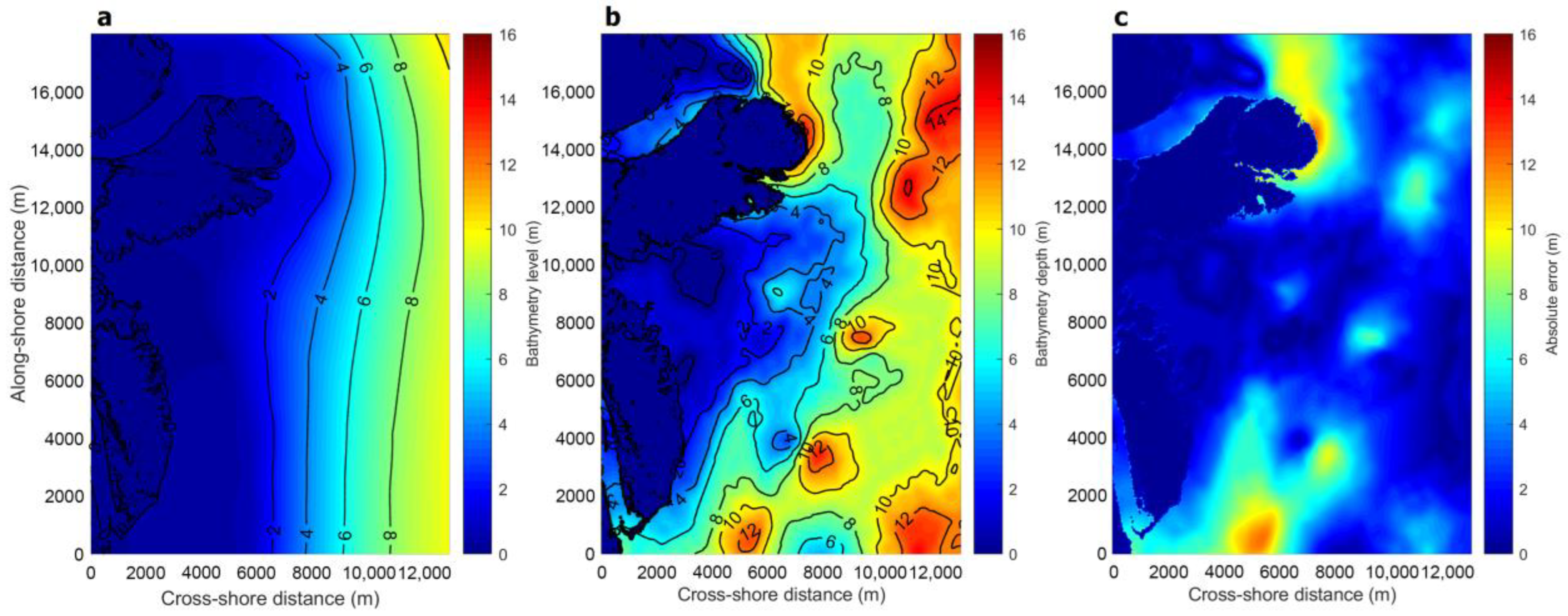
2.3. Skill Assessment of Depth Model

Several statistical methods were applied to compare the differences between the depth values extracted from the bathymetric maps with the original resolutions (NC50 and GT50) and interpolated bathymetric maps. Taking NC50 and NC10 as an example, statistical metrics, including the Bias (m), the difference of median—Diff.Md (m), the root mean square error—RMSE (m), the median absolute error—MdAE (m), and the coefficient of correlation—$R^2$, are defined as follows:

$$Bias=Mean\left(Z_{NC50}\right)-Mean\left(Z_{NC10}\right)$$

(5)

$$Diff.Md=Median\left(Z_{NC50}\right)-Median\left(Z_{NC10}\right)$$

(6)

$$RMSE=\sqrt{Mean\left({\left(Z_{NC50}-Z_{NC10}\right)}^2\right)}$$

(7)

$$MdAE=Median\left(\left|Z_{NC50}-Z_{NC10}\right|\right)$$

(8)

$$R^2=\left[{\displaystyle \sum }{\left(Z_{NC50}-Z_{NC10}\right)}^2/{\displaystyle \sum }{\left(Z_{NC50}-Mean\left(Z_{NC50}\right)\right)}^2\right]$$

(9)

where $Z_{NC50}$ and $Z_{NC10}$ correspond to the depth values extracted from bathymetric maps NC50 and NC10, respectively. These statistical criteria were applied to compare the depth values of the Chinese nautical chart-based bathymetric map with those derived from the GMRT-based map at different resolutions.

Table 1. Descriptive statistics of depth values obtained using various bathymetric maps (unit: m).

Maps	NC50	NC10	NC5	NC2	GT50	GT10	GT5	GT2
Min	−11.785	−11.815	−11.792	−11.795	−15.132	−15.214	−16.042	−16.316
Max	4.372	4.401	4.522	4.433	4.372	4.401	3.915	5.298
Median	−2.169	−2.223	−2.171	−2.173	−6.918	−6.976	−6.942	−6.949
Mean	−3.496	−3.538	−3.503	−3.505	−5.795	−5.871	−5.829	−5.833
STD	4.021	4.03	4.018	4.018	4.891	4.889	4.888	4.889
	Comparing with NC50				Comparing with GT50
Bias	-	0.0411	0.0066	0.0083	-	0.0763	0.0346	0.0388
Diff.Md	-	0.0543	0.0016	0.0041	-	0.058	0.0242	0.0313
MdAE	-	0.0252	0.0306	0.0337	-	0.0878	0.0511	0.0255
RMSE	-	0.2945	0.2568	0.2656	-	0.8605	0.615	0.7166

presents the descriptive statistics of the depth values and a comparison between the 50 m resolution bathymetric map and other interpolated maps. Generally, the data derived from the NC50 bathymetric map demonstrated a water depth interval of approximately 0–12 m, with a mean/median of 3.5/2.2 m. The depth values acquired from the GT50 over the study area ranged from 0 to ~15 m, with a mean/median of 5.8/6.9 m. There were no significant differences in the mean (i.e., bias metric) and median depth values between NC50 and the other interpolated bathymetric maps (NC10, NC5, and NC2). Comparable results were observed when comparing the GT50 to GT10, GT5, and GT2. In addition,

Table 2. Coefficient of correlation ($R^2$) matrix between depth values obtained using different bathymetric maps.

Maps	NC50	NC10	NC5	NC2	GT50	GT10	GT5	GT2
NC50	1
NC10	0.9936	1
NC5	0.998	0.9946	1
NC2	0.9979	0.9947	0.9992	1
GT50	0.8617	0.8512	0.8545	0.8538	1
GT10	0.8561	0.8547	0.8547	0.8545	0.9846	1
GT5	0.8594	0.8539	0.8575	0.8566	0.9921	0.9908	1
GT2	0.8579	0.8535	0.8568	0.8573	0.9892	0.9913	0.9958	1

shows a relatively high degree of correlation between bathymetric maps derived either from the same (above 0.99 and 0.98, for nautical chart-based and GMRT-based maps, respectively) or a different dataset (greater than 0.85 for most of the pairs). These results verify the consistency of the resampling raster function and endorse the use of interpolation to generate bathymetry with the desired resolution.

However, there is a noticeable difference between the two sources of bathymetry data, which were estimated using statistical metrics (

Table 3. Statistical comparison between the depth levels of the NC-based and GMRT-based bathymetric maps with respect to different resolutions (unit: m).

Pairs	NC50 vs. GT50	NC10 vs. GT10	NC5 vs. GT5	NC2 vs. GT2
Bias	2.2982	2.3334	2.3262	2.3287
Diff.Md	4.7487	4.7524	4.7713	4.7759
MdAE	1.6178	1.6678	1.6753	1.6608
RMSE	3.388	3.4247	3.4188	3.4157

) and it is shown in Figure 3 and Figure 4. Particularly, in Table 3, the mean and median of depth values derived from the Chinese nautical chart are shallower than that of GMRT data, with the median of absolute error being about 1.61–1.68 m and the root mean square error being about 3.38–3.42 m. To assess the spatial distribution of depth differences, Figure 3 illustrates the cross-shore profiles spaced every 2000 m, starting from 2000 to 16,000 m longshore distances, which were extracted from the NC-based and GMRT-based bathymetric maps of different resolutions. There were differences in the morphological cross-shore profiles extracted from the NC-based and GMRT-based maps, regardless of the grid resolution. The profiles obtained from the NC-based maps showed smooth morphologies from the nearshore to the offshore region, whereas complex variations in depth values were displayed by those of the GMRT-based maps. For example, when taking the NC5 and GT5 maps, a similar observation could be made quickly for the entire study area (Figure 4). Additionally, the spatial distribution of their absolute differences revealed two hot spots of large dissimilarity next to the southern and northern coasts of the delta (approximately 0–4000 m seaward from two river mouths of the Yellow River), while they showed good agreement for most parts in the center between 6000 and 12,000 m longshore distance). In this study, 9 numerical wave gauges were set up in the center region to investigate the wave dynamics.

3. Results and Discussion

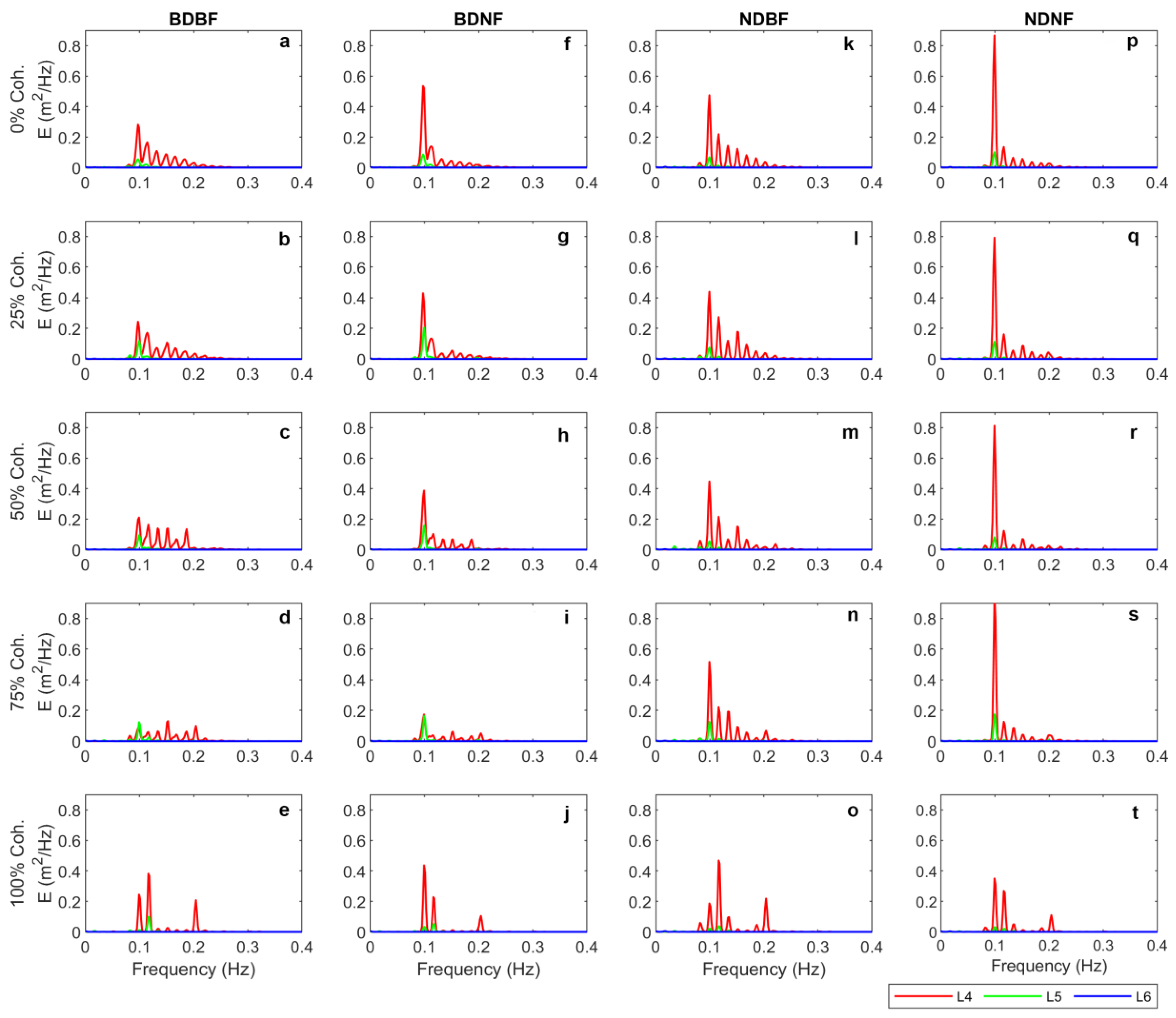
3.1. Energy Spectra Analysis

Figure 5 illustrates the energy spectra at three locations (L4, L5, and L6 in Figure 2a) for four different scenarios of incident waves (BDBF, BDNF, NDBF, and NDNF) for different levels of wave coherence. The energy spectra were calculated based on the time series of the wave height and represent the distribution of energy levels among different frequencies at specific locations. It can be noticed that the interference of the coherent waves results in discrete peaks in the energy spectra at the numerical gauges, whereas in the absence of wave coherency, the energy spectra are most like the input wave energy spectrum.

Figure 6 shows the simulated root mean square wave height ($H_{rms}$) and significant wave height ($H_{sig}$) at the longshore transect that passes the surveyed wave gauge (approximately 11,000 m cross-shore distance) with respect to different averaging periods, percentages of wave coherence, and scenarios of input energy spectra. The observation data indicated that significant (root mean square) wave height in the offshore ranged from 0.14 to 0.76 (0.13 to 0.44) m, with a mean of 0.36 (0.23) m. To study the consistency of the wave height distribution in different averaging periods, the modelled wave height was calculated using the zero-crossing method for three different time intervals: 900 s (simulation time from 4500 to 5400 s), 1800 s (from 3600 to 5400 s), and 3600 s (from 1800 to 5400 s), after a spin-up interval of 1800 s (from 0 to 1800 s). Generally, the simulated $H_{rms}$ and $H_{sig}$ variations were approximately stationary in the longshore direction and fluctuated around and above the target wave height determined according to the observed wave data. This behavior in the case of 100% coherence is in good agreement with the recent work of Zhang et al. [64]. As discussed by Zhang et al. [64], regardless of the averaging intervals used for estimating the wave height, there was no significant difference in the fluctuation patterns of longshore $H_{sig}$. However, they only analyzed $H_{sig}$ generated by the default wavemaker (i.e., 100% coherence waves). The present study has taken a further step when investigating the persistence of the longshore distributed $H_{rms}$ and $H_{sig}$ of different averaging periods with different degrees of wave coherences. For smaller degrees of coherence, particularly waves with 0% coherence, there are notable differences in the longshore fluctuation corresponding to different averaging periods. A shorter time interval resulted in a higher variation in $H_{sig}$. However, these differences were difficult to observe in average $H_{rms}$.

For the scenario where no coherent waves occur, the $H_{rms}$ distribution in the longshore variation remains approximately uniform over the domain regardless of the characteristics of the energy spectra and the interval of the averaging period, while there is a noticeable fluctuation of $H_{sig}$ considering a particularly short averaging period. In addition, the wave height with broad directional spreading presented a higher magnitude and more complex longshore distribution pattern than that with narrow-directional spreading. However, broad-frequency spreading produced fewer discontinuous peaks and gentler wave height variability than narrow-frequency spreading. These observable differences are in good agreement with the results of Salatin et al. [44] and can be explained by the distribution of energy levels and wave–wave interference of coherent waves.

Regarding the variation in the longshore wave height, for either $H_{rms}$ or $H_{sig}$, the magnitude of fluctuation is proportional to the degree of coherence. Waves with higher coherency express stronger magnitudes, varying in the longshore direction. The highest range of variation is ~0.5 m for the case of wavemaker with 100% coherence. These correlations were quantitatively evaluated using the standard deviation and variance of the longshore $H_{rms}$ and $H_{sig}$ (Figure 7 and Figure 8).

Figure 9 and Figure 10 illustrate the spatial distributions of $H_{rms}$ and $H_{sig}$ averaged for 1800 s over the entire domain with respect to different energy spectra and two specific cases of coherency levels at 0% and 100%. Generally, the wave height distribution in the longshore direction over the entire domain, regarding the type of energy spectra and degree of coherence, was like the wave height variation for a longshore transect. Without coherent waves, the generated wave height was uniformly distributed in the longshore distribution over the domain, and the decreasing of wave heights in the cross-shore direction owing to topological changes was straightforward to observe. In the scenarios with no coherent waves, the mean current speed demonstrates similar patterns for the longshore uniform domain. Furthermore, waves with BDBF energy spreading exhibited the most continuous spatial distribution of the wave height in both directions over the domain.

The maximum vorticity for each energy spectrum case at both coherency levels is shown in Figure 11. The vorticity significantly increased when the wavemaker energy changed from narrow to broad directional spreading, whereas there was no difference between the broad- and narrow-frequency spreading scenarios. Regarding the coherency effects, the vorticity for the case of non-coherent waves was homogeneously distributed throughout the domain with mostly positive values. The distribution for the other case is more complex, with varying longshore amplitudes.

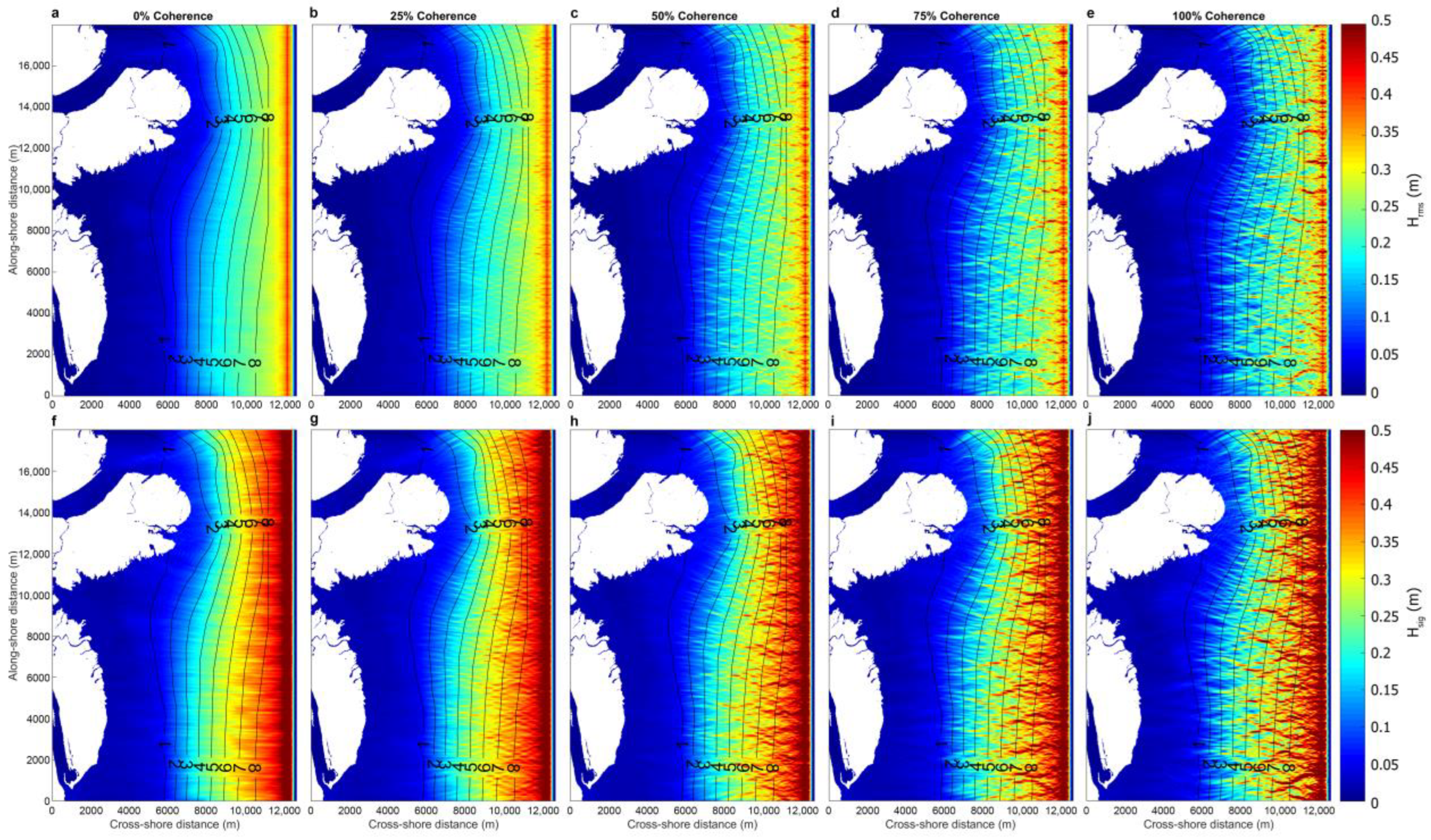
3.2. Coherence Analysis

To further investigate the impact of coherency effects, spatiotemporal variations in wave heights (Figure 12), the maximum cross-shore current velocity ($u_{max}$) and vorticity (${\sigma }_{\omega }$) were examined with respect to different degrees of coherence. The waves were generated by the newly proposed wavemaker with BDBF energy spreading and were derived for a time interval of 1800 s (simulated time from 1800 to 3600 s). Without the coherency effect, the wave height is consistently distributed over the domain owing to the uniform distribution of the energy spectra in the broad frequency-spreading scenario. Moreover, the wave components received higher energy levels in the case of broad directional spreading than in the other scenarios, resulting in stronger wave–wave interference of the coherent waves. Therefore, the longshore variation patterns of the wave height become noticeable and more complex as the components of the coherent waves increase.

The longshore transects of $H_{rms}$ and $H_{sig}$ distributions at the cross-shore distances of 8000, 10,000, and 12,000 m for the above wavemaker scenarios are demonstrated in Figure 13. By visualizing the longshore wave height at different locations in the case of no coherent waves, the impact of topography on longshore variability could be clearly observed. The results agree with the discussion by Salatin et al. [44], as wave interference becomes more intense because most of the wave energy is concentrated at a small number of frequencies and distributed in equal proportions among coherent waves with different directions, thus leading to an increase in the variation in the wave height. Furthermore, the wave components that do not propagate in the mean direction receive a high amount of energy in broad-directional spreading scenarios, thus contributing to the intricate wave–wave interference of coherent waves across the domain.

The cross-shore transects of the $H_{rms}$ and $H_{sig}$ distributions at alongshore distances of 6000, 8000, and 10,000 m for the above wavemaker scenarios are demonstrated in Figure 14a–e and Figure 14g–k, respectively. The longshore standard deviations of $H_{rms}$ and $H_{sig}$ for different degrees of wave coherence are presented in Figure 14f and Figure 14l, respectively. As the wave height was uniformly distributed in the alongshore direction of the domain for the case of 0% wave coherence, there were no significant differences among the wave heights at the varying cross-shore transects. In contrast, the existence of coherent waves in the domain leads to a complex spatial distribution of wave height, thus enhancing the fluctuation at different cross-shore transects. In addition, the magnitude of wave height variations increased proportionally with the coherency degree. Without the coherency effects, the impact of morphological changes on the wave height is readily detected as the propagating waves gradually dissipate towards the shoreline and reduce approximately half of their height (e.g., from approximately 0.4 to 0.2 m) at water depths of 5–6 m (approximately 3–4 km away from the wavemaker). The bathymetric effect on the wave height distribution was highlighted by visualizing the longshore standard deviations of $H_{rms}$ and $H_{sig}$ averaged over 1800 s in Figure 14 f and l, respectively. Despite the decrease in wave height due to bathymetric changes in the absence of wave coherence, its longshore standard deviation remains stable and negligible in the offshore zone (from X = 10,000 m and further). The standard deviation of the wave height increased when the waves traveled to the breaker zone (approximately X = 8000 m) in the northern part of the domain (from Y = 10,000 m and above) and decreased when they propagated close to the shoreline a water depth of 1 m (approximately X = 6000 m) and below. In contrast, in the presence of wave coherence, it is more difficult to investigate the underlying drivers of cross-shore and longshore variations in wave height.

Figure 15 describes the distribution of the maximum current velocity in the cross-shore direction ($u_{max}$) and the maximum instantaneous vorticity (shear wave amplitude, ${\sigma }_{\omega }$) for a time interval of 1800 s (simulated time from 1800 to 3600 s) over the domain. The instantaneous vorticity was estimated for every computational grid point throughout the domain, and the share wave amplitude at each point was demonstrated. The presence of wave coherence noticeably diminished both the uniformity of the spatial distribution and magnitude of the maximum cross-shore velocity and vorticity. Notwithstanding, the spatial pattern of the maximum cross-shore velocity was closely comparable to the distribution of the wave height over the domain, whereas the maximum vorticity showed significant differences. When waves propagated to the surf zone of the study area, where the water depth was in the range of 1–5 m, the velocity of the cross-shore current decreased, whereas the vorticity accelerated, representing a higher shear wave magnitude in this region. These observations are highlighted in Figure 16a,b through the longshore average of the maximum cross-shore velocity and vorticity, respectively. In addition, the longshore average of the maximum energy spectrum at all the numerical wave gauges was computed to study the mixed effects of varying bathymetry and coherency on the dissipation of longshore wave energy in the cross-shore direction (Figure 16c,d). There was no significant difference in energy dissipation among the studied cases of wave coherence, although the energy loss in the case of 100% coherence was slightly less than that of the other scenarios. The generated waves dissipated more than 60% of the energy when traveling to locations where the depth level was less than 5 m, dissipated more than 80% when the water depth was shallower than 2 m, and completely dissipated the energy when breaking at the shoreline.

Figure 17 presents snapshots of the surface elevation, cross-shore current velocity, and maximum vorticity field, which were captured at different simulated time steps of t = 5, 15, 30, 60, and 90 min. Waves propagated in an approximately uniform direction, followed by shoaling effects at locations where the water depths were approximately 4–5 m. In addition, the cross-shore velocity of the generated waves gradually slowed down when propagated from the offshore to the nearshore zone, slightly accelerated, and induced higher vorticity in the surf zone before breaking near the coastline (approximately at a water depth of 1 m). As the breaking of individual random waves could create vorticity, it is efficient to identify the surf and breaker zones of the YRD by observing time-varying snapshots of the maximum vorticity.

4. Conclusions

To improve the performance of the numerical model in the simulation of nearshore wave processes, it is essential to fully understand the impact of coherency effects on wave interference and spatiotemporal distribution of wave statistics over the domain. In the present study, the state-of-the-art Boussinesq-type wave model FUNWAVE-TVD was used to simulate wave propagation in the nearshore regions of the Yellow River Delta (YRD), considering different degrees of wave coherence and varying types of input energy spectra in the wavefield. The coherent waves in this study were generated using a new directional wavemaker proposed by Salatin et al. [44] and developed for the FUNWAVE-TVD model. Thus, by changing the number of coherent waves generated in the wavefield, this study clarified the impact of wave coherence on the spatial distribution of wave statistics such as the root mean square and significant wave heights, the maximum cross-shore current velocity, and vorticity. In addition, by comparing bathymetry data obtained from the Chinese nautical charts and satellite-based databases (i.e., GMRT), the authors suggest that interpolated data from nautical charts could be an alternative and acceptable approach for preparing high-resolution depth data for model simulations. The major findings of this study are summarized as follows:

(1)

Among several public satellite-based databases, the Copernicus DEM database (GLO-30) can provide 30 m resolution cell-centered grid elevation data that cover the modern topography of the YRD. Despite delivering high-quality bathymetry data with high resolution (~50 m), the latest version of GMRT (v4.0) cannot provide accurate water depths near the modern coastline of the YRD. Therefore, the derived depth data from the Chinese nautical chart at the YRD are considered to obtain accurate bathymetry at a desirable resolution, as the interpolated bathymetry is not only in good agreement with satellite-based data but also displays smooth morphologies from the offshore to the modern coastline regions, which could benefit the model simulation.

(2)

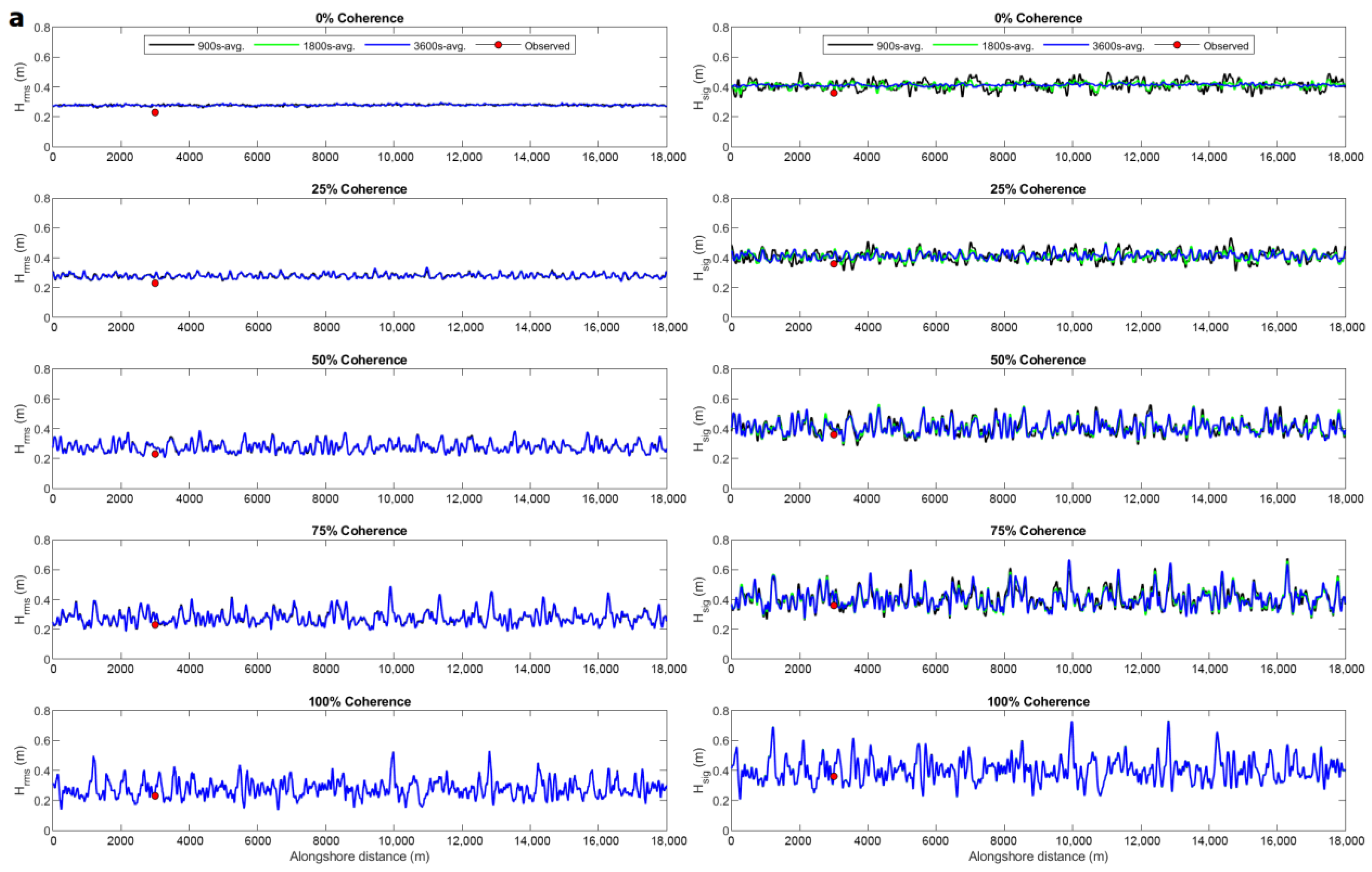
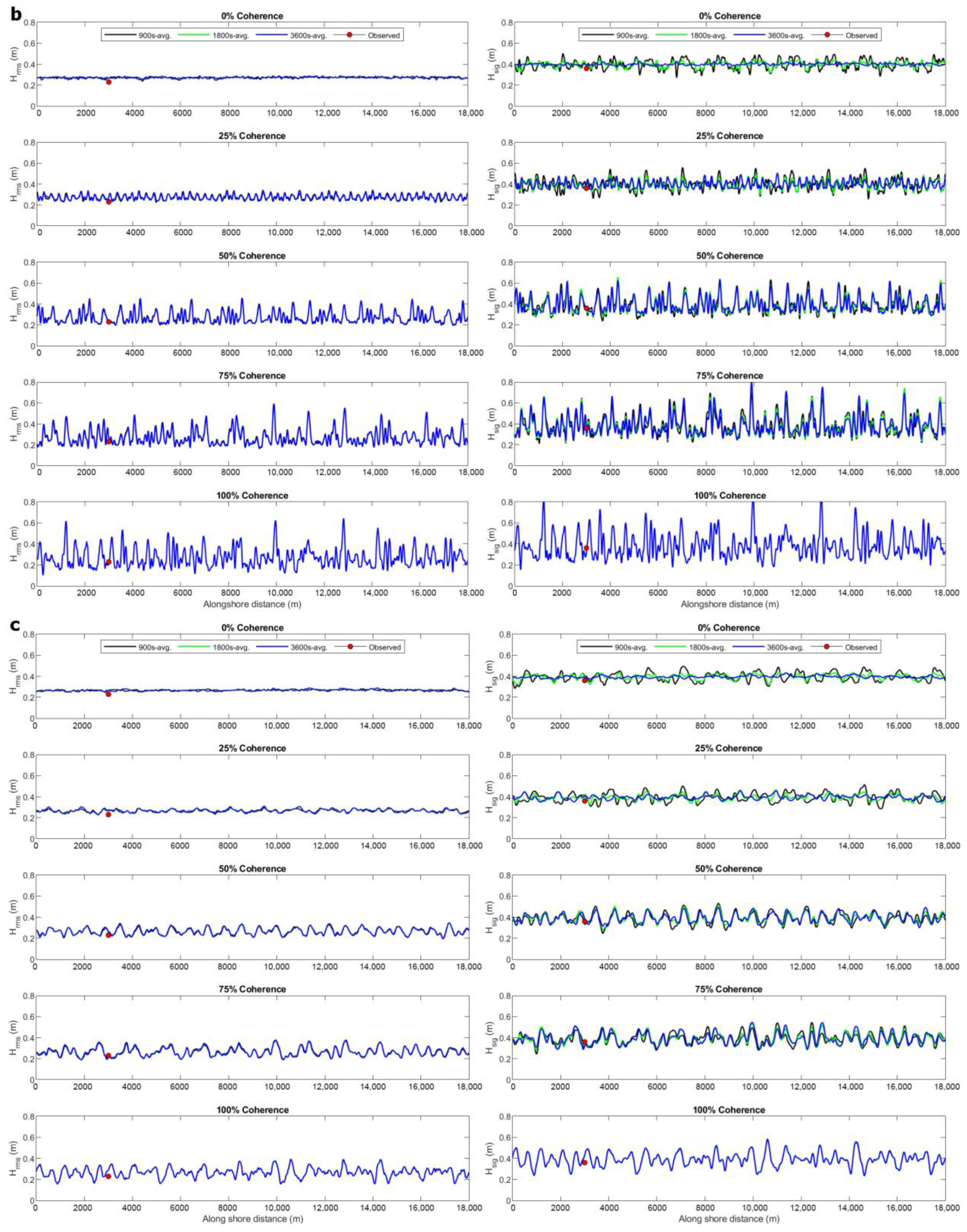
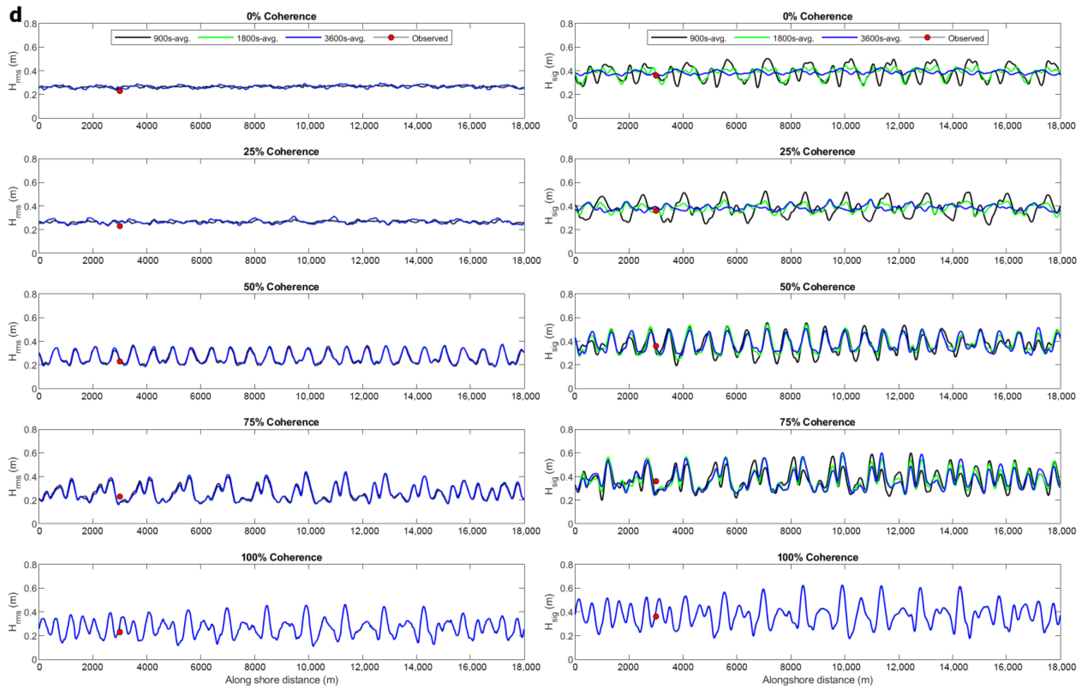
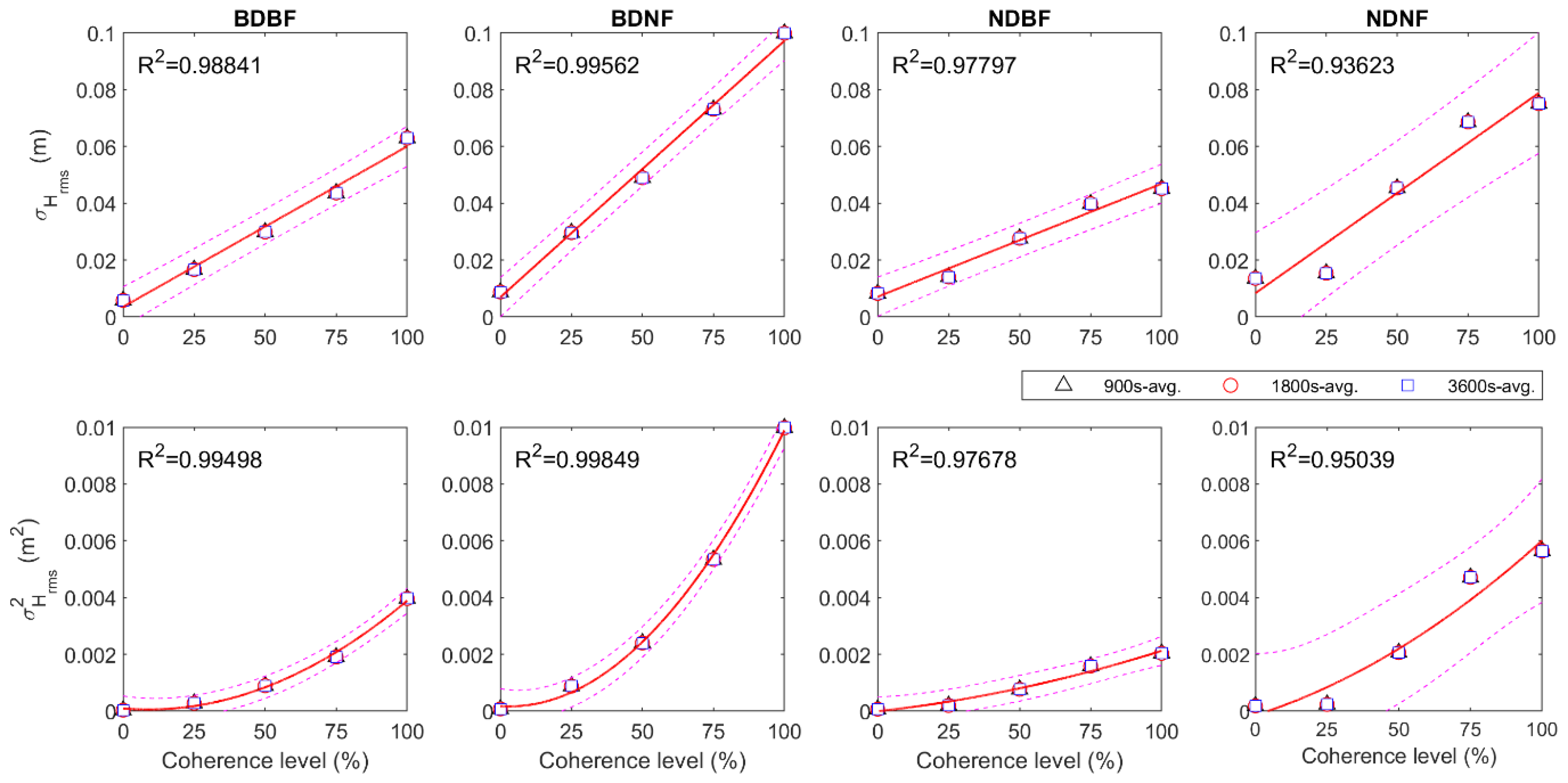
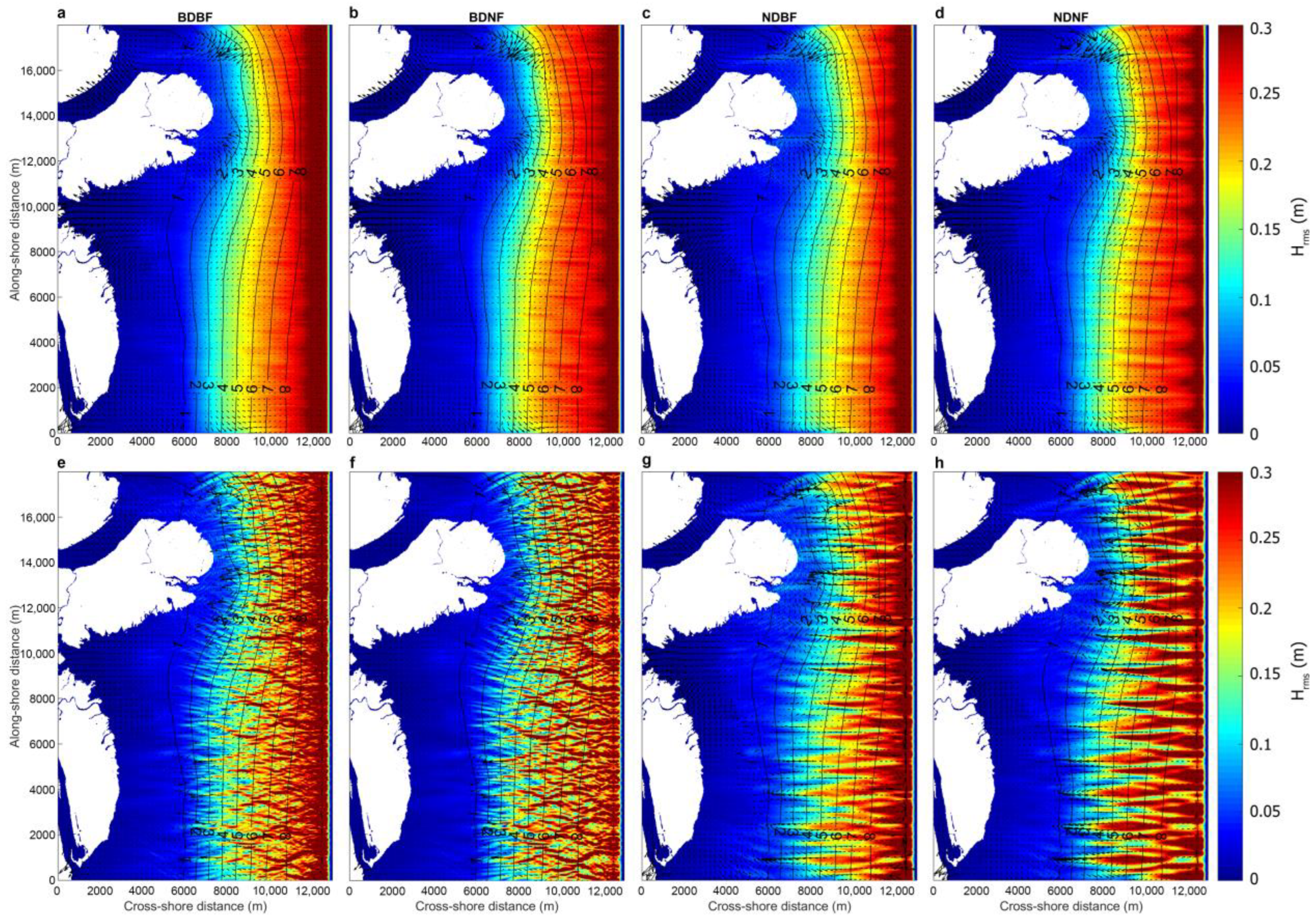
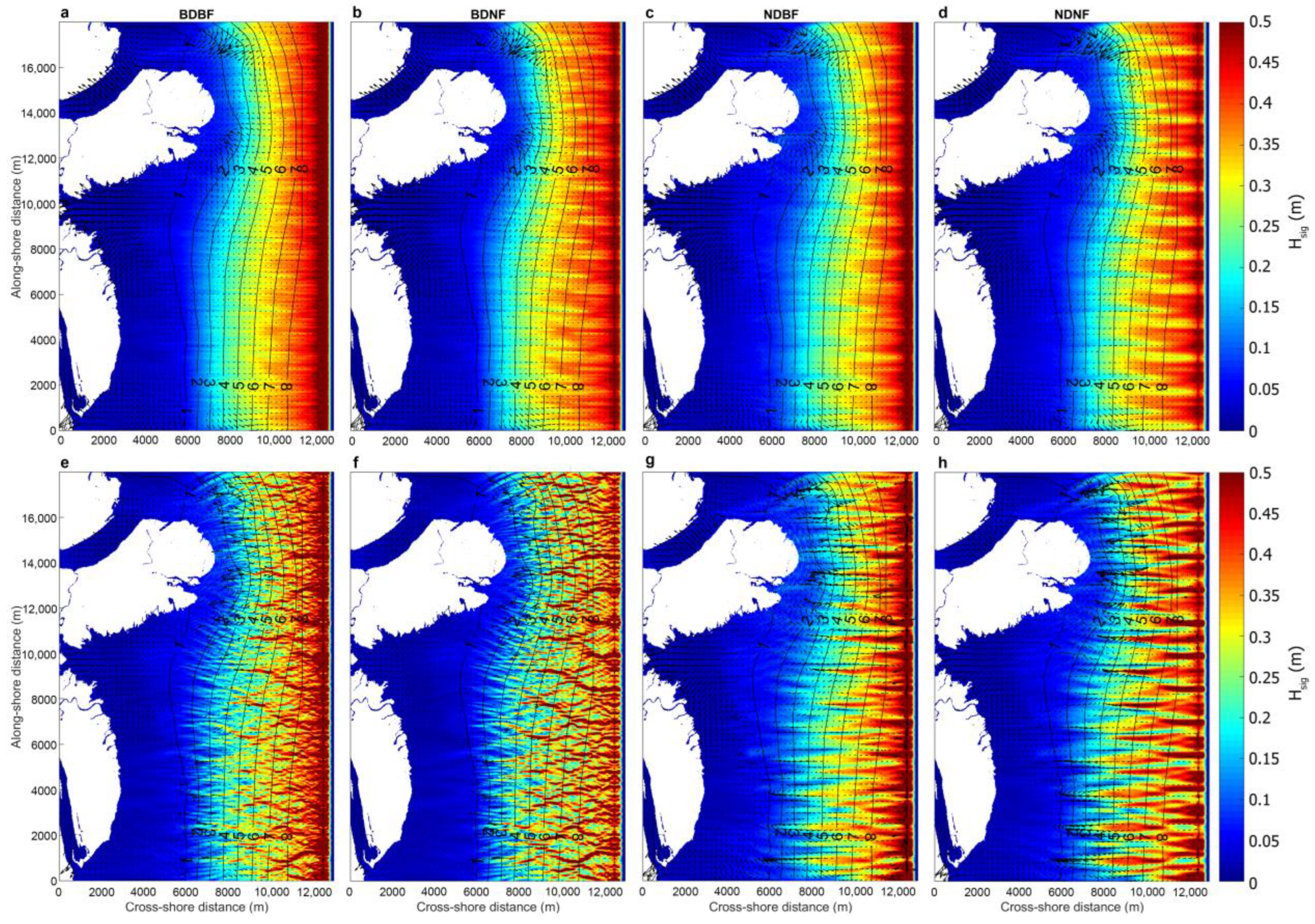
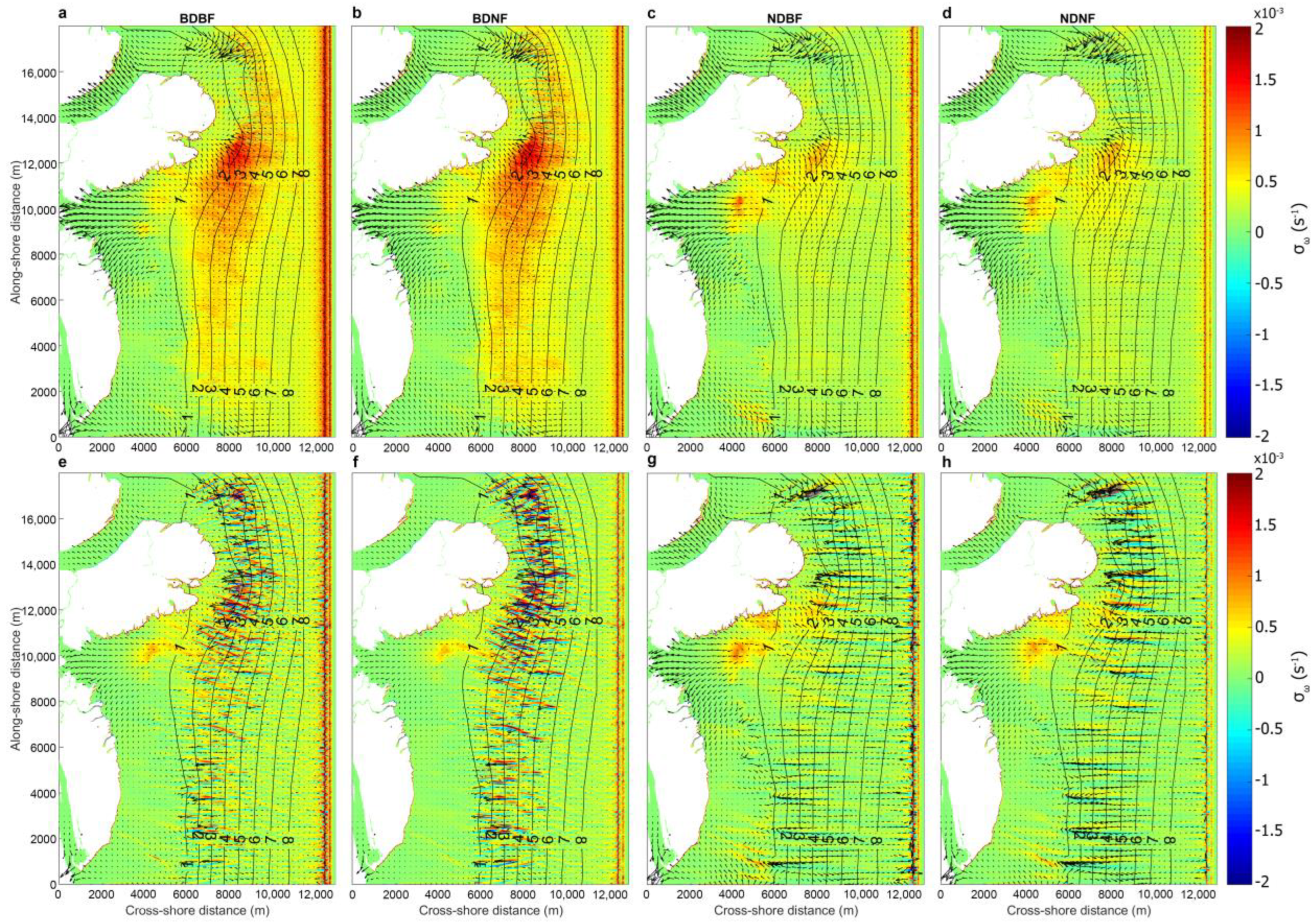
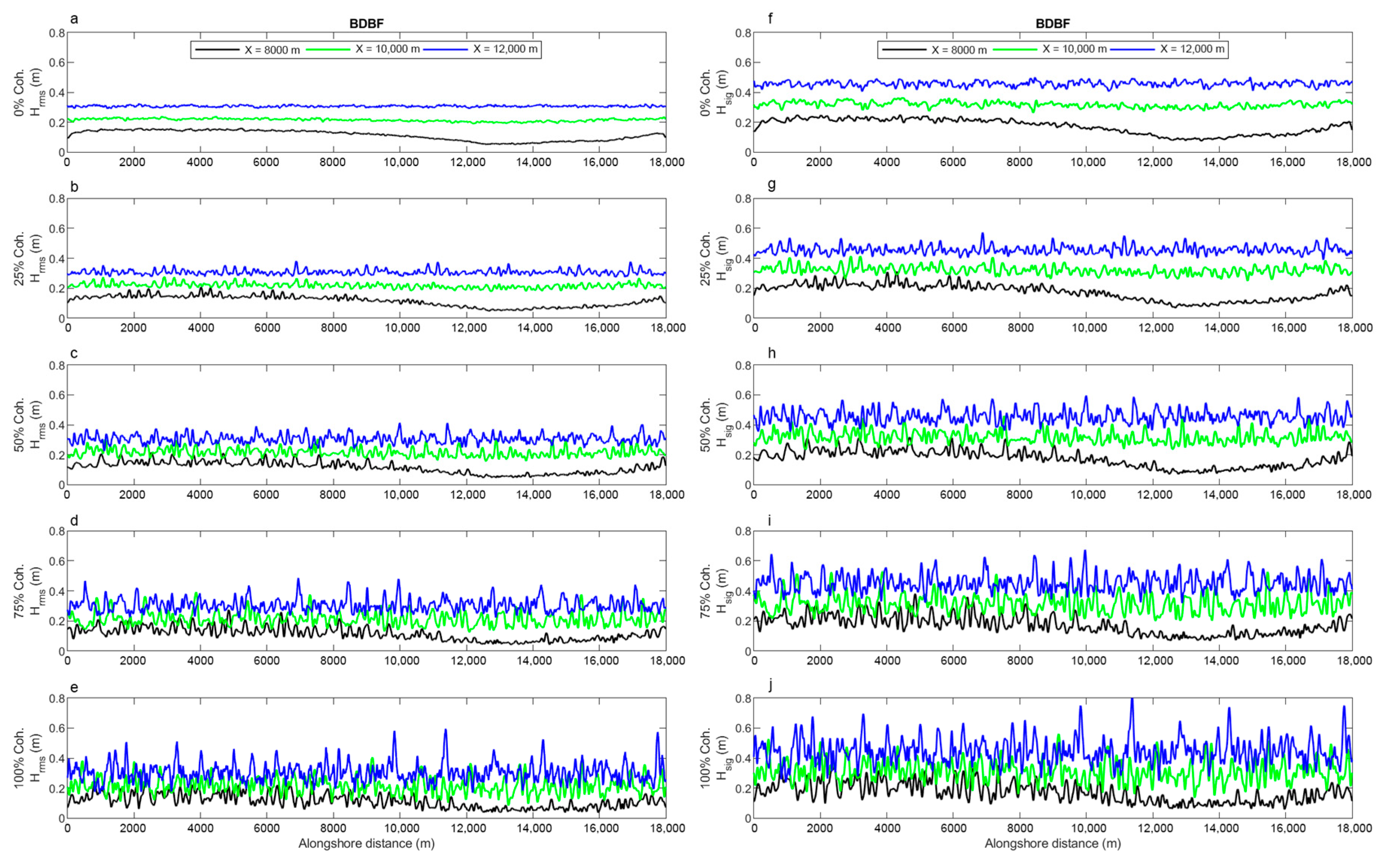
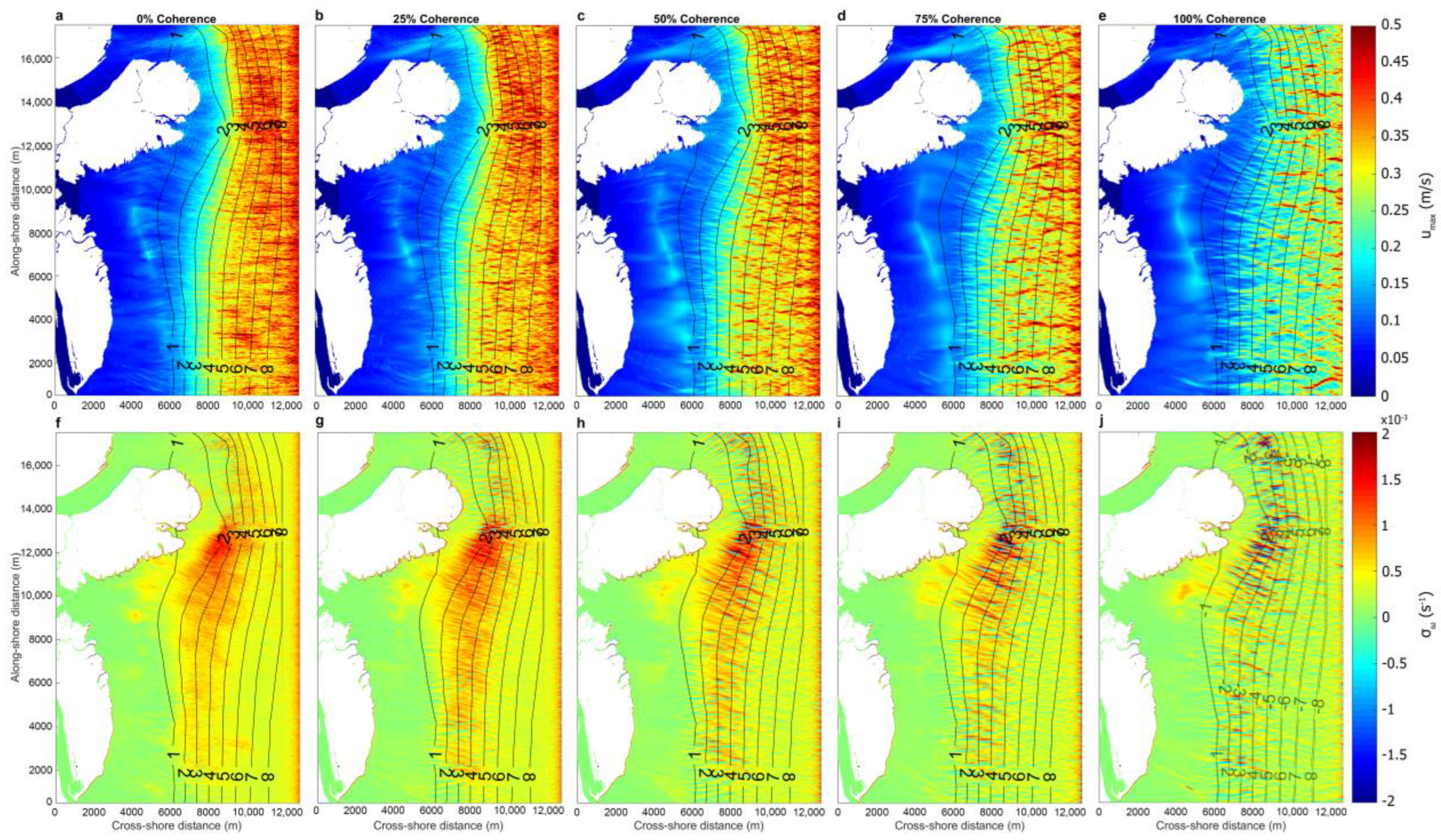
The newly proposed wave model is a suitable approach for investigating the impact of topography on wave dynamics because it can exclude coherency effects on the longshore variability of wave propagation. The generated waves with higher coherencies exhibited stronger variations in magnitude. In addition, the 1800 s averaging period of wave statistics is an applicable parameter for obtaining quality results, as in small degrees of coherence, a shorter time interval would present a higher variation in significant wave height. Additionally, the most constant spatial distribution of wave height was observed for waves with BDBF energy propagating across the domain. Although there was no difference between situations with broad and narrow frequency spreading, the vorticity increased noticeably when the wavemaker energy switched from narrow to broad directional spreading. The absence of coherent waves caused consistently distributed vorticity in the region with mostly positive values.

(3)

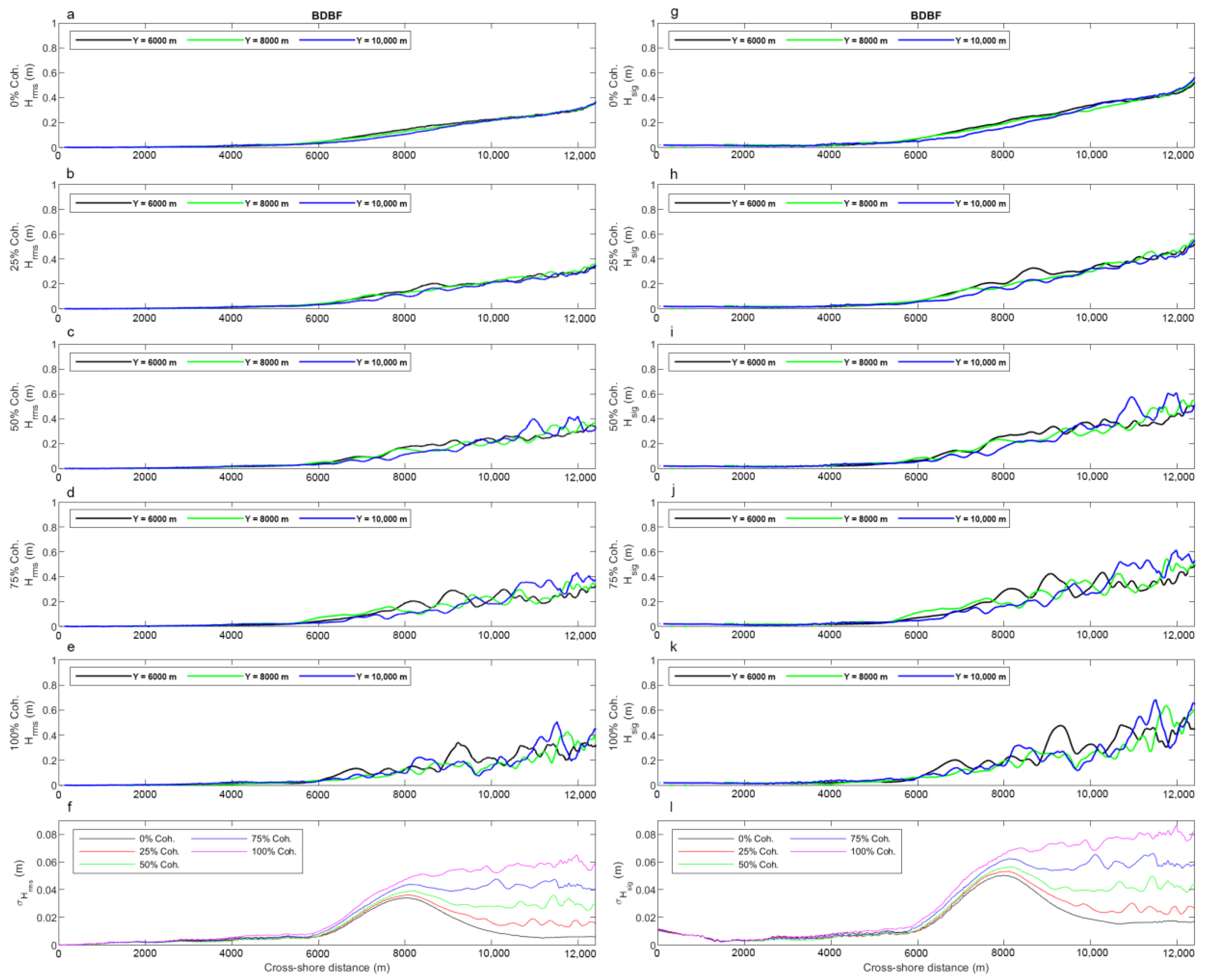
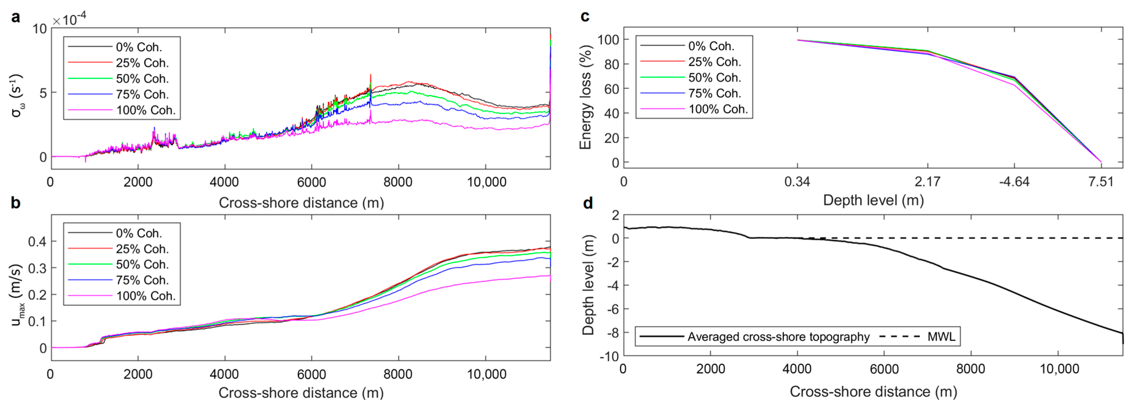
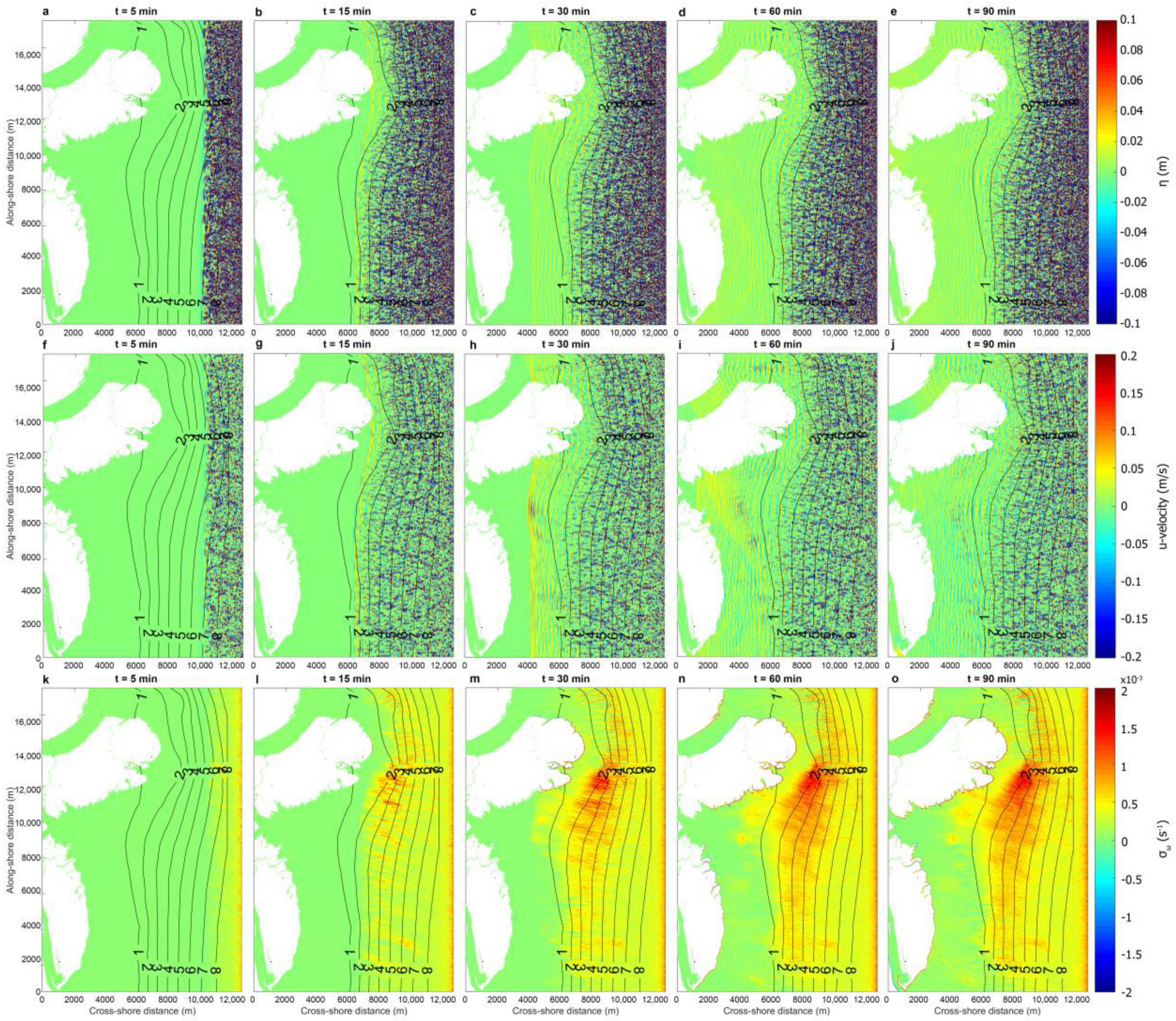
The influence of morphological changes on the wave height in the YRD is easily discernible by comparing the results with and without coherency effects, as the waves gradually dissipated when propagating toward the coastline and reduced by approximately 50% of their height (from approximately 0.4 to 0.2 m) at a water depth of 5–6 m (approximately 3–4 km away from the wavemaker). Additionally, the standard deviation of the wave height decreased when waves propagated close to the shoreline and grew as they approached the breaker zone (X $\approx$ 8000 m) in the northern half of the domain (from Y = 10,000 m and above) and decreased when waves propagated close to the shoreline at water depth of 1 m (X ≈ 6000 m) and below. The cross-shore current velocity decreases as waves move towards the surf zone of the research area, where the water depths are between 1 and 5 m, while the vorticity accelerated, indicating a higher shear wave magnitude. In the present work, time-varying snapshots of the maximum vorticity are used to efficiently identify the location of the surf and breaker zones in the YRD because the breaking of individual random waves produces a high vorticity.

(4)

Regarding energy dissipation, the analyzed degrees of wave coherence do not differ significantly in terms of energy loss, although the case of 100% coherence has a marginally lower energy loss than the other cases. In the YRD, the simulated wave dissipated more than 60% of its energy when it reached a depth of less than 5 m, more than 80% when propagated to a depth of less than 2 m, and completely dissipated the energy when it broke at the shoreline.

Consequently, by varying the degree of coherency effects and implementing different types of input energy spectra, the present study contributes to the understanding of the impact of wave coherence on the spatial distribution of wave statistics over the realistic domain when applied to the YRD. There is room for further understanding of coherency effects, particularly in terms of model improvement and field observations.

References

1. Klingbeil, K.; Lemarié, F.; Debreu, L.; Burchard, H. The numerics of hydrostatic structured-grid coastal ocean models: State of the art and future perspectives. Ocean Model. 2018, 125, 80–105. [Google Scholar] [CrossRef] [Green Version]
2. Reeve, D.E.; Chadwick, A.J.; Fleming, C.A. Coastal Engineering-Processes, Theory, and Design Practice, 3rd ed.; Taylor & Francis: London, UK; CRC Press: Boca Raton, FL, USA, 2018. [Google Scholar]
3. Feagin, R.A.; Sherman, D.J.; Grant, W.E. Coastal erosion, global sea-level rise, and the loss of sand dune plant habitats. Front. Ecol. Environ. 2005, 3, 359–364. [Google Scholar] [CrossRef]
4. Nicholls, R.J.; Hoozemans, F.M.J.; Marchand, M. Increasing flood risk and wetland losses due to global sea-level rise: Regional and global analyses. In Global Environmental Change; Elsevier Ltd.: Amsterdam, The Netherlands, 1999; pp. S69–S87. [Google Scholar] [CrossRef]
5. Fu, Y.; Guo, Q.; Wu, X.; Fang, H.; Pan, Y. Analysis and prediction of changes in coastline morphology in the Bohai Sea, China, using remote sensing. Sustainability 2017, 9, 900. [Google Scholar] [CrossRef] [Green Version]
6. Mao, M.; van der Westhuysen, A.J.; Xia, M.; Schwab, D.J.; Chawla, A. Modeling wind waves from deep to shallow waters in Lake Michigan using unstructured SWAN. J. Geophys. Res. 2016, 121, 3836–3865. [Google Scholar] [CrossRef]
7. Janssen, P. The Interaction of Ocean Waves and Wind; Cambridge University Press: Cambridge, UK, 2004. [Google Scholar] [CrossRef] [Green Version]
8. Mao, M.; Xia, M. Wave–current dynamics and interactions near the two inlets of a shallow lagoon–inlet–coastal ocean system under hurricane conditions. Ocean Model. 2018, 129, 124–144. [Google Scholar] [CrossRef]
9. Longley, K.E. Wave Current Interactions and Wave-Blocking Predictions Using Nhwave Model. Ph.D. Thesis, Naval Postgraduate School, Monterey, CA, USA, 2013; p. 61. [Google Scholar]
10. Ting, F.C.K. Laboratory study of wave and turbulence characteristics in narrow-band irregular breaking waves. Coast. Eng. 2002, 46, 291–313. [Google Scholar] [CrossRef]
11. Duran, A.; Richard, G.L. Modelling coastal wave trains and wave breaking. Ocean Model. 2020, 147, 101581. [Google Scholar] [CrossRef]
12. Gao, J.; Ji, C.; Gaidai, O.; Liu, Y.; Ma, X. Numerical investigation of transient harbor oscillations induced by N-waves. Coast. Eng. 2017, 125, 119–131. [Google Scholar] [CrossRef]
13. Gao, J.; Ma, X.; Zhang, J.; Dong, G.; Ma, X.; Zhu, Y.; Zhou, L. Numerical investigation of harbor oscillations induced by focused transient wave groups. Coast. Eng. 2020, 158, 103670. [Google Scholar] [CrossRef]
14. Gao, J.; Ma, X.; Dong, G.; Chen, H.; Liu, Q.; Zang, J. Investigation on the effects of Bragg reflection on harbor oscillations. Coast. Eng. 2021, 170, 103977. [Google Scholar] [CrossRef]
15. Liu, C.; Onat, Y.; Jia, Y.; O’Donnell, J. Modeling nearshore dynamics of extreme storms in complex environments of Connecticut. Coast. Eng. 2021, 168, 103950. [Google Scholar] [CrossRef]
16. Qu, K.; Sun, W.Y.; Deng, B.; Kraatz, S.; Jiang, C.B.; Chen, J.; Wu, Z.Y. Numerical investigation of breaking solitary wave runup on permeable sloped beach using a nonhydrostatic model. Ocean Eng. 2019, 194, 106625. [Google Scholar] [CrossRef]
17. Johnson, D.; Pattiaratchi, C. Boussinesq modelling of transient rip currents. Coast. Eng. 2006, 53, 419–439. [Google Scholar] [CrossRef]
18. Dalrymple, R.A.; MacMahan, J.H.; Reniers, A.J.H.M.; Nelko, V. Rip currents. Annu. Rev. Fluid Mech. 2011, 43, 551–581. [Google Scholar] [CrossRef]
19. Janssen, T.T.; Herbers, T.H.C. Nonlinear wave statistics in a focal zone. J. Phys. Oceanogr. 2009, 39, 1948–1964. [Google Scholar] [CrossRef]
20. Dalrymple, R.A. A Mechanism for Rip Current Generation on an Open Coast. J. Geophys. Res. 1975, 80, 3485–3487. [Google Scholar] [CrossRef]
21. Smit, P.B.; Bland, R.; Janssen, T.T.; Laughlin, B. Remote sensing of nearshore wave interference. J. Geophys. Res. 2016, 121, 3010–3028. [Google Scholar] [CrossRef] [Green Version]
22. Chawla, A.; Özkan-Haller, H.T.; Kirby, J.T. Spectral Model for Wave Transformation and Breaking over Irregular Bathymetry. J. Waterw. Port Coast. Ocean Eng. 1998, 124, 189–198. [Google Scholar] [CrossRef]
23. Dalrymple, R.A.; Lanan, G.A. Beach cusps formed by intersecting waves. Geol. Soc. Am. Bull. 1976, 87, 57–60. [Google Scholar] [CrossRef]
24. Wei, Z.; Dalrymple, R.A. SPH Modeling of Short-crested Waves. arXiv 2017, arXiv:1705.08547. [Google Scholar]
25. Spydell, M.; Feddersen, F. Lagrangian drifter dispersion in the surf zone: Directionally spread, normally incident waves. J. Phys. Oceanogr. 2009, 39, 809–830. [Google Scholar] [CrossRef]
26. Farahani, R.J.; Dalrymple, R.A.; Hérault, A.; Bilotta, G.; Rustico, E. Modeling the coherent vortices in breaking waves. In Proceedings of the 9th Internal SPHERIC Workshop, Paris, France, 3–5 June 2014. [Google Scholar]
27. Zhang, S.; Zhu, L.; Zou, K. A Comparative Study of Numerical Models for Wave Propagation and Setup on Steep Coral Reefs. China Ocean Eng. 2019, 33, 424–435. [Google Scholar] [CrossRef]
28. Smit, P.B.; Janssen, T.T. The evolution of inhomogeneous wave statistics through a variable medium. J. Phys. Oceanogr. 2013, 43, 1741–1758. [Google Scholar] [CrossRef] [Green Version]
29. Janssen, T.T.; Herbers, T.H.C.; Battjes, J.A. Evolution of ocean wave statistics in shallow water: Refraction and diffraction over seafloor topography. J. Geophys. Res. 2008, 113, 1–12. [Google Scholar] [CrossRef] [Green Version]
30. Smit, P.B.; Janssen, T.T.; Herbers, T.H.C. Stochastic modeling of coherent wave fields over variable depth. J. Phys. Oceanogr. 2015, 45, 1139–1154. [Google Scholar] [CrossRef] [Green Version]
31. Smit, P.B.; Janssen, T.T.; Herbers, T.H.C. Stochastic modeling of inhomogeneous ocean waves. Ocean Model. 2015, 96, 26–35. [Google Scholar] [CrossRef]
32. Smit, P.B.; Janssen, T.T. The evolution of nonlinear wave statistics through a variable medium. J. Phys. Oceanogr. 2016, 46, 621–634. [Google Scholar] [CrossRef]
33. Akrish, G.; Smit, P.; Zijlema, M.; Reniers, A. Modelling statistical wave interferences over shear currents. J. Fluid Mech. 2020, 891, A2. [Google Scholar] [CrossRef] [Green Version]
34. Shi, F.; Kirby, J.T.; Harris, J.C.; Geiman, J.D.; Grilli, S.T. A high-order adaptive time-stepping TVD solver for Boussinesq modeling of breaking waves and coastal inundation. Ocean Model. 2012, 43–44, 36–51. [Google Scholar] [CrossRef]
35. Liu, Z.; Fang, K.; Cheng, Y. A new multi-layer irrotational Boussinesq-type model for highly nonlinear and dispersive surface waves over a mildly sloping seabed. J. Fluid Mech. 2018, 842, 323–353. [Google Scholar] [CrossRef]
36. Liu, W.; Liu, Y.; Zhao, X. Numerical study of Bragg reflection of regular water waves over fringing reefs based on a Boussinesq model. Ocean Eng. 2019, 190, 106415. [Google Scholar] [CrossRef]
37. Liu, W.; Ning, Y.; Shi, F.; Sun, Z. A 2DH fully dispersive and weakly nonlinear Boussinesq-type model based on a finite-volume and finite-difference TVD-type scheme. Ocean Model. 2020, 147, 101559. [Google Scholar] [CrossRef]
38. Ma, G.; Kirby, J.T.; Hsu, T.J.; Shi, F. A two-layer granular landslide model for tsunami wave generation: Theory and computation. Ocean Model. 2015, 93, 40–55. [Google Scholar] [CrossRef] [Green Version]
39. Zijlema, M.; Stelling, G.; Smit, P. SWASH: An operational public domain code for simulating wave fields and rapidly varied flows in coastal waters. Coast. Eng. 2011, 58, 992–1012. [Google Scholar] [CrossRef]
40. Fang, K.; Liu, Z.; Zou, Z. Efficient computation of coastal waves using a depth-integrated, non-hydrostatic model. Coast. Eng. 2015, 97, 21–36. [Google Scholar] [CrossRef]
41. Wei, G.; Kirby, J.T.; Sinha, A. Generation of waves in Boussinesq models using a source function method. Coast. Eng. 1999, 36, 271–299. [Google Scholar] [CrossRef]
42. Goda, Y. Reanalysis of regular and random breaking wave statistics. Coast. Eng. J. 2010, 52, 71–106. [Google Scholar] [CrossRef]
43. Rijinsdorp, D.P.; Ruessink, G.; Zijlema, M. Infragravity-wave dynamics in a barred coastal region, a numerical study. J. Geophys. Res. 2015, 120, 4068–4089. [Google Scholar] [CrossRef] [Green Version]
44. Salatin, R.; Chen, Q.; Bak, A.S.; Shi, F.; Brandt, S.R. Effects of Wave Coherence on Longshore Variability of Nearshore Wave Processes. J. Geophys. Res. 2011, 126, e2021JC017641. [Google Scholar] [CrossRef]
45. Choi, Y.K.; Seo, S.N.; Choi, J.Y.; Shi, F.; Park, K.S. Wave prediction in a port using a fully nonlinear Boussinesq wave model. Acta Oceanol. Sin. 2019, 38, 36–47. [Google Scholar] [CrossRef]
46. Wang, Z.; Dong, S.; Li, X.; Soares, C.G. Assessments of wave energy in the Bohai Sea, China. Renew. Energy 2016, 90, 145–156. [Google Scholar] [CrossRef]
47. Peng, J.; Mao, M.; Xia, M. Dynamics of wave generation and dissipation processes during cold wave events in the Bohai Sea. Estuar. Coast. Shelf Sci. 2023, 280, 108161. [Google Scholar] [CrossRef]
48. Feng, J.; Li, D.; Li, Y.; Liu, Q.; Wang, A. Storm surge variation along the coast of the Bohai Sea. Sci. Rep. 2018, 8, 11309. [Google Scholar] [CrossRef] [Green Version]
49. Xu, X.; Li, X.; Chen, M.; Li, X.; Duan, X.; Zhu, G.; Feng, Z.; Ma, Z. Land-ocean-human interactions in intensively developing coastal zone: Demonstration of case studies. Ocean Coast. Manag. 2016, 133, 28–36. [Google Scholar] [CrossRef]
50. Wu, L.; Wang, J.; Gao, S.; Zheng, X.; Huang, R. An analysis of dynamical factors influencing 2013 giant jellyfish bloom near Qinhuangdao in the Bohai Sea, China. Estuar. Coast. Shelf Sci. 2017, 185, 141–151. [Google Scholar] [CrossRef]
51. Shi, C.; Zhang, D. Processes and mechanisms of dynamic channel adjustment to delta progradation: The case of the mouth channel of the Yellow River, China. Earth Surf. Process. Landf. 2003, 28, 609–624. [Google Scholar] [CrossRef]
52. You, Z.-J.; Chen, C. Coastal Dynamics and Sediment Resuspension in Laizhou Bay; Elsevier Inc.: Amsterdam, The Netherlands, 2019. [Google Scholar] [CrossRef]
53. Wei, G.; Kirby, J.T. Time-dependent numerical code for extended boussinesq equations. J. Waterw. Port Coast. Ocean Eng. 1995, 121, 251–261. [Google Scholar] [CrossRef]
54. Chen, Q. Fully nonlinear Boussinesq-type equations for waves and currents over porous beds. J. Eng. Mech. 2006, 132, 220–230. [Google Scholar] [CrossRef]
55. Kennedy, A.B.; Kirby, J.T.; Chen, Q.; Dalrymple, R.A. Boussinesq-type equations with improved nonlinear performance. Wave Motion 2001, 33, 225–243. [Google Scholar] [CrossRef]
56. Chawla, A.; Kirby, J.T. A source function method for generation of waves on currents in Boussinesq models. Appl. Ocean Res. 2000, 22, 75–83. [Google Scholar] [CrossRef]
57. Toro, E.F. Riemann Solvers and Numerical Methods for Fluid Dynamics: A Practical Introduction; Springer: Berlin/Heidelberg, Germany, 2009. [Google Scholar] [CrossRef]
58. Erduran, K.S.; Ilic, S.; Kutija, V. Hybrid finite-volume finite-difference scheme for the solution of Boussinesq equations. Int. J. Numer. Methods Fluids 2005, 49, 1213–1232. [Google Scholar] [CrossRef]
59. Gottlieb, S.; Shu, C.W.; Tadmor, E. Strong stability-preserving high-order time discretization methods. SIAM Rev. 2001, 43, 89–112. [Google Scholar] [CrossRef]
60. Malej, M.; Smith, J.M.; Salgado-Dominguez, G. Introduction to Phase-Resolving Wave Modeling with FUNWAVE; ERDC/CHL CHETN-I-87; U.S. Army Engineer Research and Development Center: Vicksburg, MS, USA, 2015. [Google Scholar]
61. Tonelli, M.; Petti, M. Hybrid finite volume—Finite difference scheme for 2DH improved Boussinesq equations. Coast. Eng. 2009, 56, 609–620. [Google Scholar] [CrossRef]
62. Mase, H.; Kirby, J.T. Hybrid frequency-domain KdV equation for random wave transformatio. In Coastal Engineering 1992; ASCE: New York, NY, USA, 1992; pp. 474–487. [Google Scholar]
63. Westcott, G. Predicting 100-Year Storm Wave’s Runup for the Coast of Rhode Island Using a Fully Nonlinear Model. Master’s Thesis, University of Rhode Island, Kingston, RI, USA, 2018; p. 1312. [Google Scholar]
64. Zhang, Y.; Shi, F.; Kirby, J.T.; Feng, X. Phase-resolved modeling of wave interference and its effects on nearshore circulation in a large ebb shoal-beach system. J. Geophys. Res. 2022, 127, e2022JC018623. [Google Scholar] [CrossRef]
Figure 1. (a) Location of the Yellow River Delta and (b) nautical chart of the study area (red box).
Jmse 11 01380 g001
Figure 2. (a) Visualization of the computational study area using an observation wave gauge (WG1) and specific cross-shore profiles at (b) Y = 10,000 m, (c) Y = 8000 m, and (d) Y = 6000 m. The bathymetry data were interpolated from a nautical chart with a 5 m resolution (NC5). The solid black strip and dotted line represent the wavemaker and sponge layer, respectively.
Jmse 11 01380 g002
Figure 3. Cross-shore profiles spaced 2 km apart were extracted from interpolated NC-based and GMRT-based bathymetric maps at different resolutions.
Jmse 11 01380 g003
Figure 4. Bathymetric contour visualizations of (a) NC5, (b) GT5, and (c) spatial distribution of their corresponding absolute errors.
Jmse 11 01380 g004
Figure 5. Energy spectra of the waves generated by the newly proposed wavemaker for (ae) BDBF, (fj) BNDF, (ko) NDBF, and (pt) NDNF scenarios at 3 locations (L4–L6) with different degrees of wave coherence.
Jmse 11 01380 g005
Figure 6. The longshore root mean square wave height H r m s (left column) and significant wave height H s i g (right column) correspond to different degrees of wave coherence generated by the newly proposed wavemaker for (a) BDBF, (b) BNDF, (c) NDBF, and (d) NDNF energy spectra.
Jmse 11 01380 g006aJmse 11 01380 g006bJmse 11 01380 g006c
Figure 7. Standard deviation and variance of the longshore root mean square wave height ( H r m s ) generated by the newly proposed wavemaker for different degrees of wave coherence and energy spectrum.
Jmse 11 01380 g007
Figure 8. Standard deviation and variance of the longshore significant wave height ( H s i g ) generated by the newly proposed wavemaker for different degrees of wave coherence and energy spectrum.
Jmse 11 01380 g008
Figure 9. Spatial distribution of the 1800 s averaged root mean square wave height ( H r m s ) generated with (top row (ad)) 0% and (bottom row (eh)) 100% wave coherence for different energy spectra.
Jmse 11 01380 g009
Figure 10. Spatial distribution of the 1800 s averaged significant wave height ( H s i g ) generated with (top row (ad)) 0% and (bottom row (eh)) 100% wave coherence for different energy spectra.
Jmse 11 01380 g010
Figure 11. Spatial distribution of the maximum vorticity ( σ ω ) generated with (top row (ad)) 0% and (bottom row (eh)) 100% wave coherence for different energy spectra.
Jmse 11 01380 g011
Figure 12. Spatial distribution of (top row (ae)) the 1800 s averaged root mean square wave height ( H r m s ) and (bottom row (fj)) significant wave height ( H s i g ) generated for the BDBF energy spectrum regarding different degrees of wave coherence.
Jmse 11 01380 g012
Figure 13. Longshore transects of (ae) 1800 s averaged root mean square wave height ( H r m s ) and (fj) significant wave height ( H s i g ) generated for the BDBF energy spectrum with respect to different degrees of wave coherence.
Jmse 11 01380 g013
Figure 14. Cross-shore transects of (ae) 1800 s averaged root mean square wave height ( H r m s ) and (gk) significant wave height ( H s i g ), along with longshore standard deviation of (f) 1800 s averaged H r m s and (l) H s i g generated for the BDBF energy spectrum with respect to different degrees of wave coherence.
Jmse 11 01380 g014
Figure 15. Spatial distributions of (top row (ae)) the maximum cross-shore current velocity ( u m a x ) and (bottom row (fj)) vorticity ( σ ω ) for the BDBF energy spectrum with different degrees of wave coherence.
Jmse 11 01380 g015
Figure 16. Longshore averages of (a) the maximum vorticity ( σ ω ), (b) maximum cross-shore current velocity ( u m a x ), and (c) energy dissipation (%) at numerical wave gauges generated with the BDBF energy spectrum of different degrees of wave coherence. Panel (d) visualized the longshore averaged topography.
Jmse 11 01380 g016
Figure 17. Spatial distributions of the time-varying (top row (ae)) surface elevation ( η ), (middle row (fj)) cross-shore current velocity ( u ), and (bottom row (ko)) maximum vorticity ( σ ω ) for the BDBF energy spectrum with 0% degree of wave coherence.
Jmse 11 01380 g017