Optimal Path Planning Method for Unmanned Surface Vehicles Based on Improved Shark-Inspired Algorithm

Abstract

As crucial technology in the auto-navigation of unmanned surface vehicles (USVs), path-planning methods have attracted scholars’ attention. Given the limitations of White Shark Optimizer (WSO), such as convergence deceleration, time consumption, and nonstandard dynamic action, an improved WSO combined with the dynamic window approach (DWA) is proposed in this paper, named IWSO-DWA. First, circle chaotic mapping, adaptive weight factor and the simplex method are used to improve the initial solution and spatial search efficiency and accelerate the convergence of the algorithm. Second, optimal path information planned by the improved WSO is put into the DWA to enhance the USV’s navigation performance. Finally, the COLREGs rules are added to the global dynamic optimal path planning method to ensure the USV’s safe navigation. Compared with the WSO, the experimental simulation results demonstrate that the path length cost, steering cost and time cost of the proposed method are decreased by 13.66%, 18.78% and 79.08%, respectively, and the improvement in path smoothness cost amounts to 19.85%. Not only can the proposed IWSO-DWA plan an optimal global navigation path in an intricate marine environment, but it can also help a USV avoid other ships dynamically in real time and meets the COLREGs rules.

1. Introduction

As small surface vehicles with autonomous navigation capability, USVs are widely used in maritime patrolling, resource exploration and marine rescue [1]. Comprehensively considering conditions such as reefs, water depth and no-sail areas, planning safe and efficient routes for USVs in a complex marine environment has gradually become a hot topic for scholars [2]. To address USV path planning issues in real marine environments, Sing et al. [3] improved the Dijkstra method and planned a global navigation path in a workspace with dynamic and static obstacles. However, the algorithm has high computational complexity and slow path search efficiency. Rui et al. [4] presented an enhanced A-star algorithm for USV path planning. The algorithm has three path smoothers, which are capable of generating a smooth and continuous path in a marine environment, but are not capable of avoiding moving obstacles in real time. Recently, some nature-inspired meta-heuristic algorithms have gradually been adopted in USV path planning. Guo et al. [5] presented an enhanced particle swarm optimization (PSO) algorithm to plan a global USV path that could avoid collisions. Cui et al. [6] enhanced the ant colony algorithm (ACO) and implemented it in USV path planning. Ma Y. et al. [7] presented a dynamic enhanced PSO, which constrained USV path planning in terms of three aspects: collision avoidance, boundary movement and speed. Sahoo et al. [8] combined the advantages of the grey wolf algorithm (GWO) and the genetic algorithm (GA) and proposed a hybrid grey wolf algorithm (HGWO) for path planning and obstacle avoidance of autonomous underwater vehicles (AUVs). Gu et al. [9] proposed an improved RRT algorithm for ship path planning, which clustered the data from an automatic identification system (AIS) and then improved the sampling strategy to accelerate convergence. The improved Douglas–Peucker (DP) and RRT algorithms are combined to optimize paths. Ma D. et al. [10] presented an enhanced Gaussian pseudospectral method (RGPM) for continuous optimal control of USVs, which can obtain an optimal smooth path. Han et al. [11] introduced a mixed approach to path planning based on enhanced Theta* and the DWA. Theta* was utilized to globally plan an optimal path and then the improved DWA was used to enhance the vehicle’s dynamic collision avoidance ability. Wang et al. [12] improved the velocity obstacle method (VO) and integrated it into the set-based guidance (SBG) framework to establish a dynamic collision avoidance (DCA) model known as USV-DCA. In order to respond to the dynamic ocean environment, Hu et al. [13] applied the A-Star algorithm and DWA method to safe USV navigation, and the real-time collision avoidance behavior of USVs conforms to COLREGs rules. Zhao et al. [14] put forward an adaptive elite GA with fuzzy inference (AEGAfi), which can control the USVs to optimize its global trajectory, and its dynamic behavior conforms to COLREGs. Li et al. [15] combined the artificial potential field (APF) with the ACO and proposed an improved APF-ACO algorithm, which overcame the local optimum shortcomings in the APF method, and achieved the path planning and collision avoidance of ships. Hao et al. [16] proposed a dynamic fast Q-learning algorithm (DFQL) to plan global USV paths in known marine environments. The algorithm initializes the Q table in combination with the APF method and provides static and dynamic rewards to motivate the USV to move toward the target point. Guo S. et al. [17] proposed a model based on deep reinforcement learning, which combined the Depth Deterministic Strategy Gradient (DDPG) algorithm with the APF method for autonomous path planning of USVs. Sang et al. [18] proposed an improved APF method and combined it with the A-Star algorithm for the formation control and path planning of the USVs.

These above researchers have carried out commendable work, however, there are still some existing problems such as falling into local optimum, time consumption and lack of smoothness in the planned path. White Shark Optimizer (WSO) is an innovative intelligent method that was developed in 2022 to imitate the foraging behavior of white sharks. Compared to other nature-inspired methods such as Butterfly Optimization Algorithm (BOA) [19], Grey Wolf Optimizer (GWO) [20], Manta Ray Foraging Optimizer (MRFO) [21], Whale Optimization Algorithm (WOA) [22] and Sparrow Search Algorithm (SSA) [23], the WSO algorithm offers the benefits of simplicity, high flexibility, strong robustness and rapid convergence [24]. However, since the population of WSO is not rich enough in its initial stage, it will decelerate the convergence in later iterations, and the risk of being caught in a local optimum should be considered. Therefore, the traditional WSO algorithm needs to be further improved. In line with the above research, this study focuses on innovative improvements and applications of WSO. When the previous literature is reviewed, the research on combining the improved WSO and DWA to solve the optimal USV path planning problem has not been found. To overcome the limitations of the traditional WSO algorithm, guide the USV to plan its global optimal path and avoid the obstacles in time, this paper proposes an enhanced WSO algorithm named IWSO-DWA, which combines the advanced techniques of circle chaotic mapping, adaptive weight factor, the simplex method and the DWA. First of all, the population of white sharks is initialized by using circle chaotic mapping to increase its diversity and speed up the algorithm’s convergence. Secondly, the adaptive weight factor method is used to update the location of the best white shark, which maintains a balance between both exploration and exploitation to promote the algorithm’s capacity. Then, the simplex method is adopted to refresh the location of white sharks as they move toward the best white shark, so as to enhance the ability of escaping the local optimal value. Finally, the enhanced DWA is utilized for avoiding obstacles dynamically. Furthermore, the azimuth evaluation function of the DWA is improved to incorporate the COLREGs rules for dynamic obstacle avoidance. By combining the improved WSO algorithm with the improved DWA method, the USV can not only sail along the optimal path, but also avoid other obstacle ships regularly in real time, and its dynamic behavior conforms to the COLREGs rule.

The following are the primary contributions of this paper:

• Aiming at insufficient search ability caused by uneven population distribution of the WSO, the white shark population is initialized by using circle chaotic mapping to enrich the diversity and enhance the initial solution quality of the algorithm.
• In the proposed IWSO, the adaptive weight factor is utilized to refresh the best white shark’s location to balance the exploration and exploitation capacity.
• To address the issue that the WSO slips into the regional optimum easily in the later iteration, the simplex method is used to update the other white sharks’ movement position toward the best white shark, which increases the probability of breaking out the local optimum.
• An innovative fusion method known as the IWSO-DWA algorithm is created by combining the improved WSO with the enhanced DWA. The proposed IWSO-DWA can not only plan a global optimal path of navigation in an intricate marine environment, but also can help USV avoid the other ships dynamically in real time and meet the COLREGs.

The rest of this paper is arranged as follows: Section 2 introduces the WSO algorithm and its improvement with multi-strategies innovatively. Then, in Section 3, both the standard DWA and its enhancement are presented. Section 4 introduces a novel global optimal path planning method called IWSO-DWA. The experimental simulation results of the IWSO-DWA are presented in Section 5, which also includes a comparison of its performance advantages with those of conventional algorithms. Section 6 concludes the research and outlines future work.

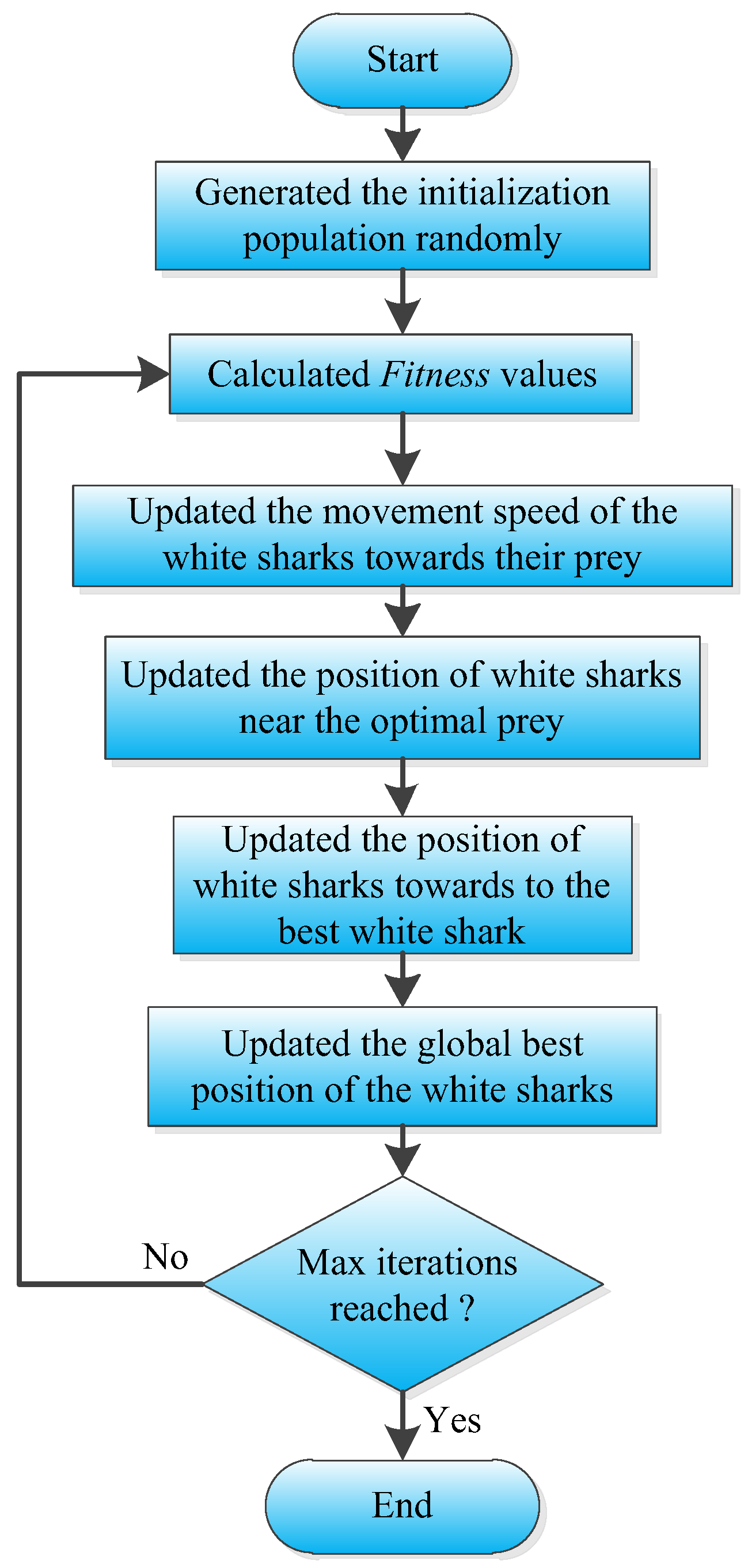
2. White Shark Optimizer and Its Improvement

2.1. Traditional White Shark Optimizer (WSO)

The White Shark Optimizer, a novel nature-inspired algorithm introduced in 2022, mimics the foraging behavior of white sharks. The WSO has the superiorities of simplicity, high flexibility and strong robustness. However, it also has certain drawbacks, including population diversity deficiency, limited search range and a tendency to slip into the regional optimum.

Assume that the set matrix of the white shark population is:

$$W={[w_1,w_2,w_3,\dots ,w_n]}^T,w_i=[w_{i,1},w_{i,2},w_{i,3},\dots ,w_{i,d}]$$

(1)

Let n denote the number of white sharks, with i = (1,2,…,n). The dimension of the problem definition is represented by the variable d.

According to Equation (1), the fitness function of white sharks is expressed as follows:

$$F(w)={[f(w_1),f(w_2),\dots ,f(w_n)]}^T$$

(2)

where $f(w_i)=[f(w_{i,1}),f(w_{i,2}),\dots ,f(w_{i,d})]$. The i-th white shark’s fitness value is represented by $f(w_i)$. The white shark population’s fitness value is denoted by $F(w)$.

In the traditional WSO algorithm, white sharks search for prey extensively through their sensitive hearing, smell and sight. While prey is moving in the sea, it will produce hesitation of the waves and special smells. Once a white shark perceives the prey’s position, it approaches the prey in a wave motion. The white sharks’ motion speed can be expressed as follows:

$$v_{k+1}^i=\mu [v_k^i+p_1({\omega }_{gbes{t}_k}-{\omega }_k^i)\times c_1+p_2({\omega }_{best}^{v_k^i}-{\omega }_k^i)\times c_2]$$

(3)

where k denotes the current iterations. $v_{k+1}^i$ is the i-th white shark’s new velocity vector in (k + 1)-th iteration. $v_k^i$ is the i-th white shark’s current velocity vector in k-th iteration. ${\omega }_{gbes{t}_k}$ denotes the white shark’s global optimal position. In the k-th step, the i-th white shark’s current position is denoted by ${\omega }_k^i$. The i-th optimal known position in the white shark population is denoted by ${\omega }_{best}^{v_k^i}$. $c_1$ and $c_2$ are selected from [0,1] randomly. $v_k^i$ denotes the white sharks’ i-th index vector when they have reached their optimal location.

Great white sharks usually hunt for food in the ocean’s depths randomly. What is more, great white sharks approach the optimal prey’s location. The location of white sharks near the optimal prey is updated as follows:

$${\omega }_{k+1}^i=\{\begin{array}{cc}{\omega }_k^i\cdot \neg \oplus {\omega }_0+u\cdot a+l\cdot b;& rand<mv\\ {\omega }_k^i+v_k^i/f;& rand\ge mv\end{array}$$

(4)

where ${\omega }_{k+1}^i$ represents the new position of i-th white shark. $\neg$ is a negation operator. The search space bound is indicated by l and u. mv represents the increasing movement force of the white shark as it approaches its prey. a,b and ${\omega }_0$ represent the vector in one dimension.

The best white shark is closely situated to the optimal prey. By using fish school behavior, all white sharks will migrate towards the best white shark, and the position is updated as follows:

$$\begin{array}{cc}{{\omega }^{\prime }}_{k+1}^i={\omega }_{gbes{t}_k}+r_1{\overrightarrow{D}}_{\omega }\mathrm{sgn}(r_2-0.5),& r_3<s_s\end{array}$$

(5)

where ${{\omega }^{\prime }}_{k+1}^i$ denotes the i-th white shark’s position relative to the prey. $\mathrm{sgn}(r_2-0.5)$ stands for the search direction of the white shark. ${\overrightarrow{D}}_{\omega }$ stands for the distance between the white shark and its prey. $s_s$ stands for the strength of white sharks’ sense organs. R₁, r₂ and r₃ are selected from [0,1] randomly.

The fish school behavior of the traditional WSO algorithm can be expressed as follows:

$${\omega }_{k+1}^i=\frac{{\omega }_k^i+{{\omega }^{\prime }}_{k+1}^i}{2\times rand}$$

(6)

where the related variables have been explained in Equations (3) and (5), so they will not be described here again.

The flow chart of the traditional WSO algorithm is depicted in Figure 1.

To sum up, the traditional WSO algorithm exhibits the following limitations:

• Since the white shark’s initialization population is created randomly, it is prone to problems such as uneven population distribution, poor diversity and low quality of the initial solution, which will not only decelerate the convergence, but also may fall into local optimum.
• Since white sharks hunt for prey amid the ocean’s depths randomly, they may not be close enough to the optimal prey, which will lead to an imbalance in both exploration and exploitation capacity.
• In the fish school behavior, other white sharks’ position may not be optimal to the best white shark, which will slip into the regional optimum easily.

2.2. Improved White Shark Optimizer (IWSO)

Due to the traditional WSO algorithm’s drawbacks, the following aspects will be improved in this paper:

• Considering the shortcomings of the WSO, such as uneven distribution and insufficient diversity of the population, a circle chaotic mapping algorithm is used to initialize the white shark population, thus further improving the quality of the initial solution.
• To address the imbalance of exploration and exploitation capacity, the adaptive weight factor method is utilized to update the best white shark’s position so that it can strengthen the balance between the exploration and exploitation capability.
• To deal with the issue that the WSO slips into the regional optimum easily, the simplex method is utilized to update the other great white sharks’ position near the best white shark to increase the possibility of the algorithm escaping the local region.

2.2.1. Circle Chaotic Mapping

Circle chaotic mapping has gained considerable attention owing to its simple structure and strong uniformity. It exhibits complex, unpredictable and random behaviors, and is often employed to enhance the diversity of the population. Circle chaotic mapping outperforms other kinds of chaotic mappings like logistic chaotic mapping and tent chaotic mapping in terms of ergodic uniformity, randomness and diversity.

In the traditional WSO algorithm, the initialization population of white sharks is generated randomly, which may lead to the disadvantages of uneven population distribution, poor diversity and slipping into the regional optimum easily in the later iteration. For this, the circle chaotic mapping method is employed to generate the initial circle population of white sharks, which is then combined with a random population. The resulting group is evaluated, and the best sharks are selected to form the optimal white shark population of the next generation. The optimized white shark individuals are more similar to the initial optimal solution than the sharks in the random population and initial circle population, which evens out white shark population distribution, broadens the algorithm’s search range and improves its efficacy.

Let $w_i$ denote the individuals within the white shark population, and then the initialization formula for the white shark population using the circle chaotic mapping method can be expressed as follows [25]:

$$w_{i+1}=mod(w_i+0.2-\frac{0.5}{2\pi }\cdot sin(2\pi \cdot w_i),1)$$

(7)

where mod indicates remainder.

2.2.2. Adaptive Weight Factor

When white sharks hunt for prey amid the ocean’s depths randomly, they may not be close enough to the optimal prey, which may lead to an imbalance between exploration and exploitation. So, the adaptive weight factor is used to update the best white shark’s position in this paper, which makes the algorithm have outstanding exploration ability in the earlier iteration and excellent exploitation ability in the later iteration. By introducing the adaptive weight factor in the process of white shark hunting prey, it is beneficial to balance the capacity for both exploration and exploitation. The adaptive weight factor proposed in this paper is expressed as follows:

$$\alpha =0.2+\frac{1}{0.6+e^{{(-f(w_i)/{\mu }^{\prime })}^k}}$$

(8)

where $f(w_i)$ represents the i-th white shark’s fitness value. ${\mu }^{\prime }$ represents the white shark’s best fitness value in the first iteration. $\alpha$ is the dynamic nonlinear factor, which is used to update the best white shark’s position. The refined formula is presented below:

$${\omega }_{k+1}^i=\{\begin{array}{cc}\alpha \cdot {\omega }_k^i\cdot \neg \oplus {\omega }_0+u\cdot a+l\cdot b;& rand<mv\\ (1-\alpha )\cdot {\omega }_k^i+v_k^i/f;& rand\ge mv\end{array}$$

(9)

As can be seen from the formula, the best white shark’s position is adjusted by the adaptive weight factor adaptively, so that the capacity for both exploration and exploitation can be balanced.

2.2.3. Simplex Method

The simplex method is a direct search algorithm for optimizing multi-dimensional unconstrained problems proposed by Nelder et al. [26] in 1965. The algorithm takes d + 1 points in d-dimensional space to form a simplex and then calculates the function value of its vertices. The sub-optimal points are obtained by internal compression, external compression, reflection and expansion of the worst point of the simplex. Then, the worst point of the simplex is replaced by the sub-optimal point, and the simplex is reconstructed to approach the global optimum continuously [27]. Since the simplex method is not affected by the continuity and derivability of the objective function, it has an excellent optimization ability, thus improving its capacity to break out the regional optimum. For this, the simplex method is utilized to update the other white sharks’ location in the fish school behavior, so as to urge them to approach the best white shark continuously and make their positions close to the global optimum, which accelerates the convergence to the optimal solution and enables it to overcome regional optimum. The diagram of the optimization process for the simplex method is shown in Figure 2.

As is shown in the figure, the optimization steps of the simplex method can be summarized as follows:

Step 1: Ranking and evaluating. All individuals of the white shark population in the d-dimensional space were ranked and evaluated for fitness values, and the current best white shark $x_g$, the second best white shark $x_b$ and the abandoned white shark $x_s$ will be selected, which is expressed as follows:

$$f(x_{d+1})\ge \dots \ge f(x_b)\ge f(x_c)=f(\frac{x_g+x_b}{2})\ge f(x_g)\ge f(x_1)$$

(10)

Step 2: Reflection. Performing a reflection operation to obtain a reflection point $x_r$. The formula of reflection operation is:

$$x_r=(1+\delta )\cdot x_c-\delta \cdot x_s$$

(11)

Here, $x_r$ refers to the reflective point obtained from $x_s$. $\delta$ is the reflective factor, typically set at 1.

Step 3: Expansion. If $f(x_g)$ > $f(x_r)$, the expansion process is carried out to obtain the expansion point $x_e$. The basic formula of expansion operation is as follows:

$$x_e=(1-\chi )\cdot x_c+\chi \cdot x_r$$

(12)

where $\chi$ is the expansion factor. If $f(x_e)$ > $f(x_r)$, substitutes $x_r$ for $x_s$.

Step 4: Outside Contraction. When $f(x_r)$ < $f(x_s)$, the outside contraction point $x_{oc}$ can be obtained by the outside contraction operation, which can be expressed as follows:

$$x_{oc}=x_c+\varphi \cdot (x_r-x_c)$$

(13)

where $\varphi$ is the contraction coefficient. If $f(x_r)$ > $f(x_{oc})$, substitutes $x_{oc}$ for $x_s$.

Step 5: Inside Contraction. If $f(x_s)$ < $f(x_r)$, the inside contraction operation can be expressed as follows:

$$x_{ic}=x_c-\varphi \cdot (x_r-x_c)$$

(14)

where $x_{ic}$ is the inside contraction point. If $f(x_{ic})$ < $f(x_s)$, substitutes $x_{ic}$ for $x_s$.

Step 6: Shrinkage. For vertices $x_i$ in d-dimensional space, the shrinkage operation is expressed as follows:

$$x_i=x_1+\xi \cdot (x_i-x_1)$$

(15)

where $\xi$ is the shrinkage coefficient.

After optimization by the simplex method, the position of the white shark individuals is closer to global optimum, which helps improve the probability of the algorithm breaking out the regional optimum.

2.2.4. Performance of IWSO on IEEE CEC-2005

In this paper, a series of advanced strategies such as circle chaotic mapping, adaptive weight factor method and simplex method is used to enhance the WSO. Moreover, the CEC-2005 test suite is used to verify the improved effect of the presented IWSO and its outstanding performance. CEC-2005 is a test suite containing several challenging benchmark functions, which has a large number of local optimal solutions, so it could be used to simulate the complexity of real search space and further verify the IWSO’s capability and reliability. The presented IWSO is compared with WSO and other five highly respected meta-heuristic algorithms such as BOA, GWO, MRFO, WOA and SSA over 25 independent runs in some benchmark functions of CEC-2005. The population size of the IWSO and other algorithms is set to 300, and the search agent is set to 50. The experimental simulation results are displayed in

Table 1. Optimization results of IWSO and other algorithms (BOA,GWO,MRFO,WOA,SSA,WSO) running on the CEC-2005 test function.

Function		BOA	GWO	MRFO	WOA	SSA	WSO	IWSO
F1	Best	9.16 × 10−6	7.19 × 10−20	2.40 × 10−269	2.20 × 10−55	0.00 × 100	7.21 × 101	0.00 × 100
	Worst	2.99 × 10−5	7.00 × 10−18	2.73 × 10−255	8.42 × 10−49	2.26 × 10−175	3.75 × 102	0.00 × 100
	Mean	2.00 × 10−5	1.80 × 10−18	1.20 × 10−256	3.44 × 10−50	9.03 × 10−177	2.25 × 102	0.00 × 100
	Std	5.34 × 10−6	1.85 × 10−18	0.00 × 100	1.68 × 10−49	0.00 × 100	7.07 × 101	0.00 × 100
F2	Best	1.85 × 10−8	8.05 × 10−12	1.14 × 10−136	1.40 × 10−35	0.00 × 100	2.78 × 100	0.00 × 100
	Worst	5.21 × 10−1	6.99 × 10−11	5.96 × 10−127	1.04 × 10−31	2.31 × 10−61	7.02 × 100	0.00 × 100
	Mean	5.52 × 10−2	1.75 × 10−11	2.71 × 10−128	1.28 × 10−32	9.24 × 10−63	4.94 × 100	0.00 × 100
	Std	1.31 × 10−1	1.27 × 10−11	1.19 × 10−127	2.66 × 10−32	4.62 × 10−62	1.17 × 100	0.00 × 100
F3	Best	8.23 × 10−6	1.17 × 10−5	4.60 × 10−261	2.10 × 104	0.00 × 100	3.76 × 102	0.00 × 100
	Worst	2.74 × 10−5	2.66 × 10−2	7.44 × 10−245	6.91 × 104	5.76 × 10−121	1.42 × 103	0.00 × 100
	Mean	1.81 × 10−5	2.73 × 10−3	6.66 × 10−246	4.73 × 104	2.31 × 10−122	8.60 × 102	0.00 × 100
	Std	4.48 × 10−6	5.69 × 10−3	0.00 × 100	1.27 × 104	1.15 × 10−121	2.75 × 102	0.00 × 100
F4	Best	1.14 × 10−3	1.54 × 10−5	1.10 × 10−136	3.57 × 10−2	0.00 × 100	6.73 × 100	0.00 × 100
	Worst	2.66 × 10−3	2.81 × 10−4	7.69 × 10−122	8.50 × 101	8.76 × 10−97	1.17 × 101	0.00 × 100
	Mean	1.81 × 10−3	8.91 × 10−5	3.25 × 10−123	4.22 × 101	3.51 × 10−98	9.04 × 100	0.00 × 100
	Std	3.89 × 10−4	5.82 × 10−5	1.54 × 10−122	2.65 × 101	1.75 × 10−97	1.35 × 100	0.00 × 100
F5	Best	2.88 × 101	2.57 × 101	2.21 × 101	2.76 × 101	2.35 × 10−9	8.02 × 102	2.87 × 10−7
	Worst	2.89 × 101	2.87 × 101	2.51 × 101	2.87 × 101	5.60 × 10−4	2.27 × 104	2.24 × 10−6
	Mean	2.89 × 101	2.67 × 101	2.35 × 101	2.80 × 101	8.45 × 10−5	7.75 × 103	1.03 × 10−6
	Std	2.47 × 10−2	7.96 × 10−1	5.87 × 10−1	3.10 × 10−1	1.50 × 10−4	5.41 × 103	1.06 × 10−6
F6	Best	3.48 × 100	9.60 × 10−5	3.32 × 10−9	7.01 × 10−2	1.99 × 10−10	5.18 × 101	9.98 × 10−9
	Worst	6.28 × 100	1.36 × 100	1.71 × 10−7	9.51 × 10−1	2.22 × 10−6	4.60 × 102	2.35 × 10−8
	Mean	4.98 × 100	6.08 × 10−1	2.70 × 10−8	3.29 × 10−1	4.36 × 10−7	2.50 × 102	1.88 × 10−8
	Std	6.48 × 10−1	3.91 × 10−1	3.38 × 10−8	2.07 × 10−1	5.68 × 10−7	1.05 × 102	7.65 × 10−9
F7	Best	8.60 × 10−4	6.36 × 10−4	2.06 × 10−5	1.49 × 10−4	5.74 × 10−6	1.55 × 10−2	1.29 × 10−5
	Worst	6.09 × 10−3	5.87 × 10−3	3.18 × 10−4	1.68 × 10−2	9.01 × 10−4	1.15 × 10−1	1.00 × 10−4
	Mean	3.13 × 10−3	2.41 × 10−3	1.57 × 10−4	3.62 × 10−3	2.88 × 10−4	4.02 × 10−2	4.56 × 10−5
	Std	1.28 × 10−3	1.24 × 10−3	8.72 × 10−5	3.36 × 10−3	2.25 × 10−4	2.27 × 10−2	4.74 × 10−5
F8	Best	−1.71 × 107	−7.42 × 103	−9.41 × 103	−1.26 × 104	−1.26 × 104	−4.11 × 103	−1.23 × 104
	Worst	−6.46 × 104	−4.57 × 103	−7.32 × 103	−7.05 × 103	−5.63 × 103	−2.94 × 103	−1.22 × 104
	Mean	−1.48 × 106	−6.18 × 103	−8.51 × 103	−9.84 × 103	−8.76 × 103	−3.40 × 103	−1.23 × 104
	Std	3.37 × 106	8.07 × 102	5.36 × 102	1.87 × 103	2.36 × 103	2.90 × 102	7.79 × 101
F9	Best	3.42 × 10−8	1.65 × 10−12	0.00 × 100	0.00 × 100	0.00 × 100	3.12 × 101	0.00 × 100
	Worst	3.58 × 10−4	2.03 × 101	0.00 × 100	5.68 × 10−14	0.00 × 100	1.73 × 102	0.00 × 100
	Mean	2.50 × 10−5	7.42 × 100	0.00 × 100	2.27 × 10−15	0.00 × 100	1.15 × 102	0.00 × 100
	Std	7.67 × 10−5	5.76 × 100	0.00 × 100	1.14 × 10−14	0.00 × 100	3.90 × 101	0.00 × 100
F10	Best	6.63 × 10−4	6.33 × 10−11	8.88 × 10−16	8.88 × 10−16	8.88 × 10−16	3.80 × 100	8.88 × 10−16
	Worst	1.87 × 10−3	6.28 × 10−10	8.88 × 10−16	1.51 × 10−14	8.88 × 10−16	6.75 × 100	8.88 × 10−16
	Mean	1.35 × 10−3	2.28 × 10−10	8.88 × 10−16	5.58 × 10−15	8.88 × 10−16	5.25 × 100	8.88 × 10−16
	Std	2.77 × 10−4	1.38 × 10−10	0.00 × 100	2.85 × 10−15	0.00 × 100	7.50 × 10−1	0.00 × 100

.

The table presents the objective function values for the IWSO and other algorithms in terms of their best, worst, average and standard deviation. Based on the results, it can be concluded that the IWSO effectively identifies the global optimum solution for the majority of the CEC-2005 test functions, and its standard deviation is smaller than that of the WSO algorithm and the other five meta-heuristic algorithms, which shows that IWSO algorithm is effective in improving WSO algorithm. Therefore, when solving complex optimization problems, the proposed IWSO algorithm is robust and reliable.

3. Dynamic Window Approach and Its Improvement

3.1. USV Modeling

Since there are many parameters in the actual USV motion model, it may be difficult to directly model it. Therefore, the following assumptions are used to simplify the USV motion model [28].

• USV is considered a rigid body with uniform mass distribution and no geometric deformation.
• The roll, pitch and heave motions of USV can be ignored.
• The xz-plane of USV is symmetrical, and the center of mass lies in the geometric symmetry plane.
• During the voyage of USV, the temporal and spatial variability of ocean currents and wind in the selected area is considered to be quasi-static.

For the DWA method, it is important to construct the motion model of USV first. According to Ref. [29], the USV has restricted mobility and its motion trajectory can be regarded as consisting of each small arc. If $\Delta t$ is very small, the motion of the USV may be modeled as a uniform linear motion. In Ref. [30], USV’s motion planning problem can be simplified to the motion of a rigid body with three freedom degrees (surge, sway and yaw) in plane space. Based on the above analysis, ignoring the influence of wind and ocean currents, USV’s model can be formulated as:

$$\{\begin{array}{l}{x}_{t+1}-x_t=v_t\cdot \Delta t\cdot \cos {\theta }_t\\ y_{t+1}-y_t=v_t\cdot \Delta t\cdot \sin {\theta }_t\\ \begin{array}{l}{\theta }_{t+1}-{\theta }_t={\omega }_t\cdot \Delta t\\ \begin{array}{c}\dot{p}=R_{\psi }(\psi )\cdot v\\ \dot{\psi }=r\end{array}\end{array}\end{array}$$

(16)

where at time t, $(x_t,y_t)$ and ${\theta }_t$ are the USV’s location and orientation, respectively. Similarly, $(x_{t+1},y_{t+1})$ and ${\theta }_{t+1}$ represent the USV’s location and orientation at time t + 1, respectively. $v_t$ represents the USV’s linear velocity at time t. ${\omega }_t$ represents the USV’s angular velocity at time t. $p={[x,y]}^T$ stands for the USV’s spatial vector. $v={[u,v]}^T$ represents the USV’s velocity vector. $R_{\psi }(\psi )$ is a rotation matrix, which is expressed by the following formula:

$$R_{\psi }(\psi )=\left[\begin{array}{cc}\cos \psi & -\sin \psi \\ \sin \psi & \cos \psi \end{array}\right]$$

(17)

The USV’s motion model is displayed in Figure 3.

3.2. Velocity Sampling

Due to countless groups $(v,\omega )$ in the domain of motion vectors, sampling these velocities based on the real USV restrictions is required to obtain a workable velocity range [31].

• Speed constraint: limited by the USV’s maximal and minimal velocity:

$$V_m=\{(v,\omega )|v\in [v_{\min },v_{\max }],\omega \in [{\omega }_{\min },{\omega }_{\max }]\}$$

(18)

where the minimal and maximal linear velocities are represented by $v_{\min }$ and $v_{\max }$, respectively. The minimal and maximal angular velocities are represented by ${\omega }_{\min }$ and ${\omega }_{\max }$, respectively.

2.

Dynamic constraint: influenced by the motor acceleration and deceleration performance of USV, which is expressed as follows:

$$V_d=\{(v,\omega )|v\in [v_g-{v_f}^{\prime }\cdot \Delta t,v_g+{v_e}^{\prime }\cdot \Delta t]\wedge \omega \in [{\omega }_g-{{\omega }_f}^{\prime }\cdot \Delta t,{\omega }_g+{{\omega }_e}^{\prime }\cdot \Delta t]\}$$

(19)

where $v_g,{\omega }_g$ represents the USV’s current linear and angular velocity, respectively. ${v_e}^{\prime },{{\omega }_e}^{\prime }$ represent the USV’s maximal linear acceleration and maximal angular acceleration, respectively. ${v_f}^{\prime },{{\omega }_f}^{\prime }$ represent the USV’s maximal linear deceleration and maximal angular deceleration, respectively.

3.

Braking distance constraint: To prevent the USV from colliding with other ships or obstacles, the USV will be constrained by the braking distance, and the speed will be reduced to zero within the braking distance according to its maximum deceleration. The braking distance constraint is presented in the following formula:

$$V_a=\{(v,\omega )|v\le {\sqrt{2\cdot dist(v,\omega )\cdot v_f}}^{\prime }\wedge \omega \le {\sqrt{2\cdot dist(v,\omega )\cdot {\omega }_f}}^{\prime }\}$$

(20)

where $dist(v,\omega )$ stands for the distance between the nearest obstacle to the USV and the end of the deduced trajectory.

3.3. Evaluation Function and Its Improvement

After sampling the velocity of USV, the DWA method will deduce the trajectory based on the sampled velocity, and the scoring mechanism is used to sort these trajectories, and the greatest score trajectory will be selected as the final trajectory of USV. Among them, the scoring mechanism of the DWA method is composed of three functions, speed function, azimuth evaluation function and obstacle distance function [32], which are expressed as follows:

$$F\left(v,\omega \right)=\alpha \cdot vel\left(v,\omega \right)+\beta \cdot head\left(v,\omega \right)+\gamma \cdot dist\left(v,\omega \right)$$

(21)

where $\alpha$, $\beta$ and $\gamma$ are the weight factor of the three functions. However, owing to the absence of knowledge on the global path, the DWA method is prone to slip into the regional optimum when encountering a complex marine environment. Therefore, global path information planned by the IWSO will be incorporated into the enhanced DWA method, so that the USV can break out the regional optimum.

Aiming at the shortcomings of the traditional DWA, some strategies are used to improve it in this paper. Firstly, $head(v,\omega )$ is changed to the tangent angle between the global optimal navigation path and the USV. Then, the current azimuth angle from the USV to the nearest sub-target point can be expressed by the following formula:

$${\theta }_c=tan(\frac{y_2-y_1}{x_2-x_1})\cdot \frac{{180}^{°}}{\pi }$$

(22)

where ${\theta }_c$ represents the current azimuth of the USV. $(x_1,y_1)$ represents the current position coordinates of USV. $(x_2,y_2)$ represents the position coordinates of the sub-target point nearest the USV. What is more, the improved azimuth cost function is expressed as follows:

$$hea{d}^{\prime }\left(v,\omega \right)=\left|{\theta }_c-{\theta }_{st}\right|$$

(23)

where ${\theta }_{st}$ represents the azimuth between the predicted trajectory and the target point. The improved azimuth evaluation function can guide USV along the global optimal path planned by the IWSO while avoiding other obstacle ships or dynamic obstacles.

Secondly, in order to hasten USV arrival at the target point, the distance cost function within the USV’s present location and the sub-target point is constructed, which is expressed as follows:

$$path(v,\omega )=\sqrt{{(x_E-x_{ST})}^2+{(y_E-y_{ST})}^2}$$

(24)

where $(x_E,y_E)$ represents the sub-target point coordinates. $(x_{ST},y_{ST})$ represents the current predicted trajectory coordinates.

To sum up, the assessment function for the enhanced DWA is:

$$F^{\prime }\left(v,\omega \right)=\sigma (\alpha \cdot vel\left(v,\omega \right)+\beta \cdot hea{d}^{\prime }\left(v,\omega \right)+\gamma \cdot dist\left(v,\omega \right)+\eta \cdot path(v,\omega ))$$

(25)

where $\sigma$ represents the smoothing factor. $\eta$ represents path cost weight coefficient.

4. The Proposed Fusion Algorithm IWSO-DWA

To further smooth the USV’s navigation path and endow it with the ability of real-time dynamic collision avoidance, this paper combines the proposed IWSO algorithm with the improved DWA method and proposes a novel global dynamic optimal path planning method, which is named IWSO-DWA. Due to the complex maritime navigation environment and many ships coming and going, the COLREGs is introduced in this paper to construct the collision avoidance model of USV, so that it can avoid other obstacle ships reasonably while navigating along the optimal path globally. The pseudo-code of the proposed IWSO-DWA is illustrated in Algorithm 1.

Algorithm 1: IWSO-DWA

Input: The set of population size: P; The map information: G; The maximum number of iterations: $K$. Output: Optimal navigation path. 1. Initializing population by circle chaotic mapping; 2. While k < K do 3. Updating the parameters of WSO; 4. Identifying the current optimal solution; 5. for i = 1 to P do 6. Updating the motion velocity of white sharks; 7. end for 8. for i = 1 to P do 9. Refreshing the best white shark’s location by the adaptive weight factor; 10. end for 11. for i = 1 to P do 12. If rand $\le$ss then 13. ${\overrightarrow{D}}_{\omega }=\left|rand\times ({\omega }_{gbes{t}_k}-{\omega }^i{}_k)\right|$; 14. If i ==1 then 15. ${\omega }^i{}_{k+1}={\omega }_{gbes{t}_k}+r_1{\overrightarrow{D}}_{\omega }\mathrm{sgn}(r_2-0.5)$; 16. else 17. ${{\omega }^{\prime }}_{k+1}^i={\omega }_{gbes{t}_k}+r_1{\overrightarrow{D}}_{\omega }\mathrm{sgn}(r_2-0.5)$; 18. ${\omega }^i{}_{k+1}=\frac{{\omega }^i{}_k+{{\omega }^{\prime }}_{k+1}^i}{2\times rand}$; 19. end if 20. end if 21. Using the simplex method to update the white sharks’ position; 22. end for 23. Modifying the position of any white shark that exceeds the boundary; 24. Assessing and revising the updated positions; 25. k = k + 1; 26. end while 27. Obtaining the optimal path globally and incorporating it into DWA; 28. Considering the COLREGs rules; 29. return optimal navigation path.

As can be seen from the pseudo-code of the proposed IWSO-DWA, the IWSO is responsible for planning the global optimal path under a given environment model. The global optimal path information is obtained to choose the present route’s start point and sub-target point, and fed into the local path planner subsequently. Under the action of the IWSO-DWA algorithm, USV can travel along the global optimal path planned by the IWSO, and the other obstacle ships will be detected in real time as the process proceeds. When other obstacle ships approach, USV will avoid it in real time, and its dynamic behavior meets the COLREGs. After successful collision avoidance, USV will continue to move along the global optimal path. Finally, refresh the current path’s status until the USV reaches the final target point. The flow chart of IWSO-DWA for global dynamic optimal path planning is displayed in Figure 4.

4.1. COLREGs Rules

The International Regulations for Preventing Collisions at Sea (COLREGs) is a kind of sea traffic regulation that aims to avoid collisions between ships navigating the open seas.

According to Ref. [33], there are four representative rules of COLREGs: overtaking, head-on, port side crossing and starboard crossing. The four representative rules of COLREGs are shown in Figure 5.

The blue pentagon stands for USV, the red pentagon stands for obstacle ship, and the yellow oval dotted line stands for the shape range of the ship. In the overtaking situation, both USV and obstacle ship move from bottom to top. When the USV is behind the obstacle ship and on the same route, USV can overtake the obstacle ship from the port side or starboard. In the head-on situation, the obstacle ship moves from top to bottom, while the USV sails from bottom to top and meets the front of the obstacle ship, and USV can avoid the obstacle ship through starboard. In the port side crossing situation, the obstacle ship moves from left to right, while the USV sails from bottom to top and meets the obstacle ship. At this time, the obstacle ship has the obligation to avoid a collision. However, if the red dynamic obstacle ship (OS) fails to take relevant collision avoidance actions, USV should adjust the starboard in time to avoid collision with it. When the red dynamic obstacle is far away, the USV continues to move to the target point. In the starboard crossing situation, when the obstacle ship moves from right to left and the USV moves from bottom to top and meets the obstacle ship, the obstacle ship has no obligation to avoid a collision at this time. The USV needs to adjust the starboard and quickly cross the obstacle ship to avoid collision with it.

4.2. Complexity Analysis

An algorithm’s time complexity might be determined by the magnitude of the input problem (d), the population size (n), the algorithm’s iterations (K) and the cost function evaluation (c). In this paper, the total time complexity of the IWSO-DWA algorithm can be expressed as:

$$\begin{array}{ll}O\left(\mathrm{IWSO}\text{-}\mathrm{DWA}\right)& =O\left(optimalpathproblem\right)+O\left(initialization\right)\\ & +O\left(costfunctionevaluation\right)+O\left(Solutionupdate\right)\\ & =O\left(1+d\cdot n+n\cdot c\cdot K+d\cdot n\cdot K\right)\\ & \cong O\left(n\cdot c\cdot K+d\cdot n\cdot K\right)\end{array}$$

(26)

5. Experimental Results and Analysis

5.1. Environment Modeling

To replicate the intricate navigational marine conditions for USV simulation purposes, two map environment models of USV are established, both of which are 500 m × 500 m. The light blue arrow represents the direction of ocean currents, the black block represents the islands, the heavy blue triangle represents the starting point of USV with the coordinate (10,10), and the red star represents the target point of USV with the coordinate (490,490), as shown in Figure 6.

Additionally, the experiment was simulated on a laptop with an Intel(R) Core(TM) i7-5500 processor clocked at 2.40 GHz, 8 GB memory and Windows 7 64-bit operating system with MATLAB R2017b software.

5.2. Static Path Planning Simulation Experiment

There are two sets of static path planning simulation experiments to validate the proposed IWSO-DWA’s advantages in the USV’s path planning problems. The static path planning simulation experiment of USV is carried out by using the proposed IWSO-DWA, IWSO, WSO and five other common meta-heuristic algorithms (BOA, GWO, MRFO, WOA and SSA) in the same map. The parameters of the DWA part of the proposed IWSO-DWA are set as follows: The maximal linear velocity $v_{\max }$ is 5 m/s and the maximal angular velocity ${\omega }_{\max }$ is 60 rad/s. The minimal linear velocity $v_{\min }$ is 1 m/s and the minimal angular velocity ${\omega }_{\min }$ is 10 rad/s. The maximal linear acceleration $v_e^{\prime }$ is 0.7 m/s² and the maximal angular acceleration ${\omega }_e^{\prime }$ is 75 rad/s². The maximal linear deceleration $v_f^{\prime }$ is 0.8 m/s² and the maximal angular deceleration ${\omega }_f^{\prime }$ is 80 rad/s². The weight $\alpha$, $\beta$ and $\gamma$ of the evaluation function are set to 0.3, 0.06 and 0.4, respectively. The population size of white sharks and five other meta-heuristic algorithms are all set to 50, and the maximal iteration is set to 300. The mentioned algorithms (BOA, GWO, MRFO, WOA, SSA, WSO, IWSO and IWSO-DWA) are used for the static path planning of USV in the ENV.1, and the results obtained from the simulation experiment are displayed in Figure 7.

When taking into account the metrics of path length, steering times, path smoothness and time cost systematically, the static path planning performance of IWSO-DWA proposed in this study surpasses that of IWSO, WSO and other meta-heuristic algorithms (BOA, GWO, MRFO, WOA, SSA). Compared with the WSO, the path length, steering times and time cost planned by the IWSO decreased by 16.12%, 28.57% and 76.97%, respectively. And the path smoothness planned by the IWSO is improved by 30.22%.

Since the proposed IWSO-DWA algorithm is based on the IWSO algorithm to increase its dynamic characteristics, the proposed IWSO-DWA algorithm and the IWSO algorithm have equivalent effects on convergence performance when solely focusing on their static characteristics. Thus, when analyzing the algorithm’s convergence, it suffices to only evaluate the IWSO. The convergence curves of the mentioned algorithms (BOA, GWO, MRFO, WOA, SSA, WSO and IWSO) in ENV.1 are displayed in Figure 8.

In the convergence curves, the horizontal axis label represents the iteration of the algorithms, and the vertical axis represents the fitness value of the algorithms. When compared with the WSO and five other meta-heuristic algorithms, the proposed IWSO algorithm has demonstrated the fastest convergence speed and highest accuracy of final convergence accuracy.

Based on its demonstrated performance, the second group of static path planning simulation experiments is executed to further validate the advancements of the proposed IWSO-DWA. The mentioned algorithms (BOA, GWO, MRFO, WOA, SSA, WSO, IWSO and IWSO-DWA) are utilized in the static path planning simulation experiment in ENV.2, and the results are illustrated in Figure 9.

Similarly, when synthetically considering measurement criteria such as path length, steering times, path smoothness, and time cost, the proposed IWSO-DWA algorithm exhibited superior performance in the static path planning simulation experiments compared to the IWSO, the WSO and the five other meta-heuristic algorithms (BOA, GWO, MRFO, WOA and SSA). Compared with the WSO, the path length, steering times and time cost planned by the IWSO are decreased by 11.2%, 9% and 81.19%, respectively. Meanwhile, the path smoothness planned by the IWSO is improved by 9.49%. The convergence curves of the mentioned algorithms (BOA, GWO, MRFO, WOA, SSA, WSO, IWSO) in ENV.2 are shown in Figure 10.

In the convergence curves, the horizontal axis label represents the iteration of the algorithms and the vertical axis represents the fitness value of the algorithms. When compared with the WSO and five other meta-heuristic algorithms, the proposed IWSO algorithm reaches stability in about 15 iterations, which excelled in both convergence speed and accuracy.

After the completion of two static path planning simulation experiment sets, it is necessary to summarize the performance of the BOA, GWO, MRFO, WOA, SSA, WSO and IWSO algorithms in numerical format. Supposed the planned path of the algorithms can be represented by a group of points set L, and $L=\left\{L_1,L_2,\dots ,L_{\lambda }\right\}$. $\lambda$ is the number of path points in the set L. Then, the continuous steering angle between the path point L_i and the subsequent path point L_i+1 is denoted by θ_i. To better assess the smoothness of the path planned by the mentioned algorithms, a path smoothness cost metric denominated mot has been established, which is defined as follows:

$$mot={\displaystyle \sum _{i=1}^{\lambda -1}\frac{\epsilon \cdot \pi \cdot {\theta }_i}{180\cdot {(1+{\theta }_{i+1})}^{\frac{3}{2}}}}$$

(27)

where i = 1,2,…, $\lambda -1$. $\epsilon$ is the number of turns of the L. θ_i+1 is the next rotation angle of the continuous rotation angle θ_i. The smaller the value of mot, the smoother the path.

In addition, to better evaluate the optimal path planning performance of the proposed algorithm, some metrics such as the steering cost, planning time cost and shortest path length cost are considered as the measure criteria of the mentioned algorithms. The steering cost indicates the total number of turns of the path planned by the algorithms. The planning time cost refers to the time it takes for an algorithm to plan its path in a static obstacle environment. The shortest path length cost means that the algorithm plans the shortest safe and collision-free path from the starting point to the target point, which can be defined as follows:

$$C_L=C_{safe}\cdot {\displaystyle \sum _{i=2}^{\lambda }\sqrt{{(x_{L_i}-x_{L_{i-1}})}^2+{(y_{L_i}-y_{L_{i-1}})}^2}}$$

(28)

where $C_L$ represents the shortest path length cost, which is the sum of the Euclidean distances between the points $L_{i-1}$ and $L_i$ in the set L of path points planned by the algorithms. $C_{safe}$ represents the safety path cost. In this paper, all the paths provided by the algorithms must be safe and collision-free, so here, $C_{safe}=1$.

In summary, the simulation experiments of the static path planning demonstrate that the proposed IWSO-DWA can effectively plan an optimal path globally that is both secure and smooth in the established environmental models, irrespective of any changes to the distribution of obstacles. As the proposed IWSO-DWA algorithm enhances its dynamic qualities based on the IWSO algorithm, it can be deemed equivalent to the IWSO algorithm when solely considering the static characteristics of path planning. Thus, when summarizing the simulation comparison experiments of the static path planning in digital form, it only needs to compare the performance of the proposed IWSO with WSO and five other algorithms (BOA, GWO, MRFO, WOA and SSA). The algorithms’ performance in the simulation comparison experiments of the static path planning is summarized in

Table 2. Comparison performance of the mentioned algorithms (BOA, GWO, MRFO, WOA, SSA, WSO, IWSO).

ENV. Model		Metrics	Shortest Path Length Cost (m)	Steering Cost	Smoothness Cost (mot)	Time Cost (s)
	Algorithm
ENV.1	BOA		914.530	8	0.591	2.056
	GWO		802.370	9	0.456	6.564
	MRFO		777.267	11	0.794	1.920
	WOA		801.650	8	0.455	7.037
	SSA		862.133	5	0.628	3.472
	WSO		847.487	7	0.309	5.416
	IWSO		710.873	5	0.215	1.247
ENV.2	BOA		1144.975	19	3.097	7.846
	GWO		996.773	11	0.947	2.228
	MRFO		950.803	11	0.930	2.256
	WOA		941.590	11	0.977	3.355
	SSA		959.620	15	2.220	6.317
	WSO		1044.975	11	1.024	5.490
	IWSO		927.925	10	0.926	1.033

.

5.3. Dynamic Avoidance Simulation Experiment

Two sets of dynamic collision avoidance simulation experiments were conducted to validate whether the proposed IWSO-DWA conforms to COLREGs rules and effectively avoids collisions in dynamic scenarios. Four situations are established in environmental model 1 and environmental model 2 of the COLREGs respectively: overtaking situation, head-on situation, port side crossing situation and starboard crossing situation. In the figures, the blue boat indicates the USV and the red boat indicates the obstacle ship. In ENV.1, the overtaking situation between the USV and the red obstacle ship is shown in Figure 11.

The starting coordinate of the red dynamic obstacle ship is (260,120), and it moves in a straight line from bottom to top at a velocity of 2 m/s. The coordinate of the starting point of USV is (260,30), the target point of USV is (260,380), and it moves in a straight line from bottom to top at a velocity of 4 m/s. In the overtaking situation, when encountering the red dynamic obstacle ship, the USV initiates collision avoidance by veering toward the upper right direction at an angle of approximately 65 degrees. It expertly navigates past the red dynamic obstacle ship from its starboard side and continues towards the target point, following a previous path, thereby successfully avoiding a rear-end collision, and the dynamic collision avoidance behavior of the USV conforms to the COLREGs. The x, y position and yaw angle of the USV for its dynamic collision avoidance behavior are depicted in Figure 12.

After completing the overtaking situation of USV in ENV.1, the head-on situation experiment of USV is carried out, and the results are displayed in Figure 13.

The starting point coordinate of the red dynamic obstacle ship is (260,350), and it moves in a straight line from top to bottom with a moving speed of 3 m/s. The coordinate of the starting point of USV is (260,30), the target point of USV is (260,380), and it moves in a straight line from bottom to top with a moving speed of 4 m/s. In the head-on situation, when encountering the red dynamic obstacle ship, the USV initiates adjusting starboard of the ship in a direction approximately 70 degrees towards the upper right direction, then skillfully navigates past the red dynamic obstacle ship’s upper region from the USV’s starboard side. After successfully avoiding the head-on collision with the red dynamic obstacle ship, the USV then progresses toward the target point, and the dynamic collision avoidance behavior of the USV conforms to the COLREGs. The x, y position and yaw angle of the USV for its dynamic collision avoidance behavior are depicted in Figure 14.

After completing the head-on situation of USV in ENV.1, the port side crossing situation experiment of USV is carried out, and the results are displayed in Figure 15.

The starting point coordinate of the red dynamic obstacle ship is (180,110), and it moves in a straight line from left to right with a moving speed of 4 m/s. The coordinate of the starting point of USV is (260,30), the target point of USV is (260,180), and it moves in a straight line from bottom to top with a moving speed of 4 m/s. In the port side crossing situation, since the red dynamic obstacle ship is a giving way vessel, it should stop to let the USV pass when it encounters the USV. However, if the red dynamic obstacle ship did not stop, the USV must take evasive action to prevent a collision. When the red obstacle ship enters the evasive range, the USV actively adjusts the starboard and keeps a safe distance from the red obstacle ship. After collision avoidance, the USV continued to move along the original path to the target point, thus finishing the port side crossing situation, and the dynamic collision avoidance behavior of the USV conforms to the COLREGs. The x, y position and yaw angle of the USV for its dynamic collision avoidance behavior are depicted in Figure 16.

After completing the port side crossing situation of USV in ENV.1, the starboard crossing situation experiment of USV is carried out, and the results are displayed in Figure 17.

The starting coordinate of the red dynamic obstacle ship is (330,110), and it moves in a straight line from right to left with a moving speed of 4 m/s. The coordinate of the starting point of USV is (260,30), the target point of USV is (260,180), and it moves in a straight line from bottom to top with a moving speed of 4 m/s. In the starboard crossing situation, since the USV is a giving way vessel, it should stop to let the red dynamic obstacle ship pass when it encounters the red dynamic obstacle ship. When the red obstacle ship enters the evasive range, the USV adjusts its starboard side at approximately 47 degrees to avoid the red dynamic obstacle vessel and stops to wait for it to move away from the evasive range. Once the red obstacle vessel is out of the evasive range, the USV continues to move to the upper left to the target point, thus finishing the starboard crossing situation of the USV, and the dynamic collision avoidance behavior of USV conforms to the COLREGs. The x, y position and yaw angle of the USV for its dynamic collision avoidance behavior are depicted in Figure 18.

Similarly, in ENV.2, four dynamic avoidance simulation experiments were conducted to validate the effectiveness of the proposed IWSO-DWA in line with the COLREGs. The overtaking situation between the USV and the red dynamic obstacle ship is shown in Figure 19.

The starting point coordinate of the red dynamic target obstacle is (130,260), and it moves in a straight line from bottom to top with a moving speed of 2.5 m/s. The coordinate of the starting point of USV is (130,180), the target point of USV is (130,380), and it moves vertically upwards at a velocity of 4 m/s. In the overtaking situation, when the USV enters the evasive range, it avoids collision by steering approximately 68 degrees to the upper right and proactively sails across the upper section of the red dynamic obstacle ship from the USV’s port side. Once it safely overtakes the red dynamic obstacle ship, the USV proceeds to advance toward the target point in the upper left direction, thus finishing the overtaking situation between the USV and the red dynamic obstacle ship, and the dynamic collision avoidance behavior of the USV conforms to the COLREGs. The x, y position and yaw angle of the USV for its dynamic collision avoidance behavior are depicted in Figure 20.

After completing the overtaking situation of USV in ENV.2, the head-on situation experiment of USV is carried out, and the results are displayed in Figure 21.

The starting point coordinate of the red dynamic obstacle ship is (130,350), and it travels vertically downwards at a velocity of 2 m/s. The coordinate of the starting point of USV is (130,180), the target point of USV is (130,380), and it moves vertically upwards at a speed of 4 m/s. In the head-on situation, when the USV encounters the red dynamic obstacle ship, the USV avoids the collision by turning approximately 63 degrees to the starboard and proceeding to cross the upper section of the red dynamic obstacle ship. Once it is far away from the red dynamic obstacle ship, the USV moves to the target point in the direction of around 18 degrees to the upper left, thus finishing the head-on situation between the USV and the red dynamic obstacle ship, and the dynamic collision avoidance behavior of the USV conforms to the COLREGs. The x, y position and yaw angle of the USV for its dynamic collision avoidance behavior are depicted in Figure 22.

After completing the head-on situation of USV in ENV.2, the port side situation experiment of USV is carried out, and results are displayed in Figure 23.

The starting point coordinate of the red dynamic obstacle ship is (75,260), it moves in a straight line from left to right with a moving speed of 3 m/s. The coordinate of the starting point of USV is (130,180), the target point of USV is (130,380), and it moves in a straight line from bottom to top with a moving speed of 4 m/s. In the port side situation, since the red obstacle ship is a giving way vessel when encountering the USV, it should stop to let the USV pass. However, if the red dynamic obstacle ship did not stop, the USV should take evasive action to prevent a collision. When the red obstacle ship enters the evasive range, the USV adjusts its starboard at roughly 80 degrees to avoid the red obstacle ship. Once the USV moves away from the red obstacle ship, it continues to move to the upper left towards the target point, thus finishing the port side situation between the USV and the red dynamic obstacle ship, and the dynamic collision avoidance behavior of the USV conforms to the COLREGs. The x, y position and yaw angle of the USV for its dynamic collision avoidance behavior are depicted in Figure 24.

After completing the port side situation of USV in ENV.2, the starboard situation experiment of USV is carried out, and the results are displayed in Figure 25.

The starting point coordinate of the red dynamic obstacle ship is (200,260), and it moves in a straight line from right to left with a moving speed of 3 m/s. The coordinate of the starting point of USV is (130,180), the target point of USV is (130,380), and it moves in a straight line from bottom to top at a velocity of 4 m/s. In the starboard situation, since the USV is a giving way vessel when encountering the red obstacle ship, it should stop to let the red dynamic obstacle ship pass. When the red obstacle ship enters the evasive range, the USV steers away from collision by adjusting its starboard and maintaining a safe distance from the red obstacle ship. Once the red obstacle ship is far away, the USV crosses the upper section of the red dynamic obstacle ship and moves to the target point in the upper left direction, thus finishing the starboard situation between the USV and the red dynamic obstacle ship, and the dynamic collision avoidance behavior of the USV conforms to the COLREGs. The x, y position and yaw angle of the USV for its dynamic collision avoidance behavior are depicted in Figure 26.

6. Conclusions and Future Work

This research proposes a new IWSO-DWA algorithm to address the optimal path planning issue for USV. First of all, aiming at the disadvantages of uneven distribution and insufficient diversity of the white shark population, a circle chaotic mapping algorithm is employed to improve the initial solution’s quality. Then, the adaptive weight factor technique is used to update the best white shark’s position, ensuring a balance between global exploration and local exploitation. Furthermore, the simplex method is used to update the other white sharks’ position near the best white shark, enhancing the algorithm’s ability to escape the local optimum solution. Finally, a novel global dynamic optimal path planning method called the IWSO-DWA algorithm is developed by combining the improved WSO and the enhanced DWA. The performance of the IWSO-DWA algorithm is tested through two sets of static path planning simulation comparison experiments and two sets of dynamic avoidance simulation experiments. The study found that the IWSO-DWA algorithm outperformed traditional WSO algorithms and five other heuristic algorithms (BOA, GWO, MRFO, WOA and SSA) in the simulation experiments. Thus, the proposed IWSO-DWA algorithm not only addresses the issues encountered in the traditional WSO algorithm, but also guides USV to plan a global optimal path in challenging marine environments and possesses path smoothing capability and dynamic collision avoidance ability, and its collision avoidance behavior conforms to the COLREGs. However, the proposed IWSO-DWA has only been evaluated through simulations, and future research is required to focus on assessing its effectiveness in practical engineering optimization problems in real USV.

References

1. Bai, X.; Li, B.; Xu, X.; Xiao, Y. A Review of Current Research and Advances in Unmanned Surface Vehicles. J. Mar. Sci. Appl. 2022, 21, 47–58. [Google Scholar] [CrossRef]
2. Zhou, C.; Gu, S.; Wen, Y.; Du, Z.; Xiao, C.; Huang, L.; Zhu, M. The review unmanned surface vehicle path planning: Based on multi-modality constraint. Ocean Eng. 2020, 200, 107043. [Google Scholar] [CrossRef]
3. Singh, Y.; Sharma, S.; Sutton, R.; Hatton, D. Towards use of Dijkstra Algorithm for Optimal Navigation of an Unmanned Surface Vehicle in a Real-Time Marine Environment with results from Artificial Potential Field. TransNav Int. J. Mar. Navig. Saf. Sea Transp. 2018, 12, 125–131. [Google Scholar] [CrossRef]
4. Song, R.; Liu, Y.; Bucknall, R. Smoothed A* algorithm for practical unmanned surface vehicle path planning. Appl. Ocean Res. 2019, 83, 9–20. [Google Scholar] [CrossRef]
5. Guo, X.; Ji, M.; Zhao, Z.; Wen, D.; Zhang, W. Global path planning and multi-objective path control for unmanned surface vehicle based on modified particle swarm optimization (PSO) algorithm. Ocean Eng. 2020, 216, 107693. [Google Scholar] [CrossRef]
6. Cui, Y.; Ren, J.; Zhang, Y. Path Planning Algorithm for Unmanned Surface Vehicle Based on Optimized Ant Colony Algorithm. IEEJ Trans. Electr. Electron. Eng. 2022, 17, 1027–1037. [Google Scholar] [CrossRef]
7. Ma, Y.; Hu, M.; Yan, X. Multi-objective path planning for unmanned surface vehicle with currents effects. ISA Trans. 2018, 75, 137–156. [Google Scholar] [CrossRef]
8. Sahoo, S.P.; Das, B.; Pati, B.B.; Garcia Marquez, F.P.; Segovia Ramirez, I. Hybrid Path Planning Using a Bionic-Inspired Optimization Algorithm for Autonomous Underwater Vehicles. J. Mar. Sci. Eng. 2023, 11, 761. [Google Scholar] [CrossRef]
9. Qiyong, G.; Rong, Z.; Jialun, L.; Chen, L. An improved RRT algorithm based on prior AIS information and DP compression for ship path planning. Ocean Eng. 2023, 279, 114595. [Google Scholar] [CrossRef]
10. Ma, D.; Hao, S.; Ma, W.; Zheng, H.; Xu, X. An optimal control-based path planning method for unmanned surface vehicles in complex environments. Ocean Eng. 2022, 245, 110532. [Google Scholar] [CrossRef]
11. Han, S.; Wang, L.; Wang, Y.; He, H. A dynamically hybrid path planning for unmanned surface vehicles based on non-uniform Theta* and improved dynamic windows approach. Ocean Eng. 2022, 257, 111655. [Google Scholar] [CrossRef]
12. Wang, W.; Du, J.; Tao, Y. A dynamic collision avoidance solution scheme of unmanned surface vessels based on proactive velocity obstacle and set-based guidance. Ocean Eng. 2022, 248, 110794. [Google Scholar]
13. Hu, S.; Tian, S.; Zhao, J.; Shen, R. Path Planning of an Unmanned Surface Vessel Based on the Improved A-Star and Dynamic Window Method. J. Mar. Sci. Eng. 2023, 11, 1060. [Google Scholar] [CrossRef]
14. Zhao, L.; Bai, Y.; Paik, J.K. Global-local hierarchical path planning scheme for unmanned surface vehicles under dynamically unforeseen environments. Ocean Eng. 2023, 280, 114750. [Google Scholar] [CrossRef]
15. Li, M.; Li, B.; Qi, Z.; Li, J.; Wu, J. Optimized APF-ACO Algorithm for Ship Collision Avoidance and Path Planning. J. Mar. Sci. Eng. 2023, 11, 1177. [Google Scholar] [CrossRef]
16. Bing, H.; He, D.; Zheping, Y. A path planning approach for unmanned surface vehicles based on dynamic and fast Q-learning. Ocean Eng. 2023, 270, 113632. [Google Scholar] [CrossRef]
17. Guo, S.; Zhang, X.; Zheng, Y.; Du, Y. An Autonomous Path Planning Model for Unmanned Ships Based on Deep Reinforcement Learning. Sensors 2020, 20, 426. [Google Scholar] [CrossRef] [Green Version]
18. Sang, H.; You, Y.; Sun, X.; Zhou, Y.; Liu, F. The hybrid path planning algorithm based on improved A* and artificial potential field for unmanned surface vehicle formations. Ocean Eng. 2021, 223, 108709. [Google Scholar] [CrossRef]
19. Arora, S. Butterfly optimization algorithm: A novel approach for global optimization. Soft Comput. 2019, 23, 715–734. [Google Scholar] [CrossRef]
20. Mirjalili, S.; Mirjalili, S.M.; Lewis, A. Grey Wolf Optimizer. Adv. Eng. Softw. 2014, 69, 46–61. [Google Scholar] [CrossRef] [Green Version]
21. Zhao, W.; Zhang, Z.; Wang, L. Manta ray foraging optimization: An effective bio-inspired optimizer for engineering applications. Eng. Appl. Artif. Intell. 2020, 87, 103300. [Google Scholar] [CrossRef]
22. Mirjalili, S.; Lewis, A. The Whale Optimization Algorithm. Adv. Eng. Softw. 2016, 95, 51–67. [Google Scholar] [CrossRef]
23. Xue, J.; Shen, B. A novel swarm intelligence optimization approach: Sparrow search algorithm. Syst. Sci. Control Eng. 2020, 8, 22–34. [Google Scholar] [CrossRef]
24. Braik, M.; Hammouri, A.; Atwan, J.; Al-Betar, M.A.; Awadallah, M.A. White Shark Optimizer: A novel bio-inspired meta-heuristic algorithm for global optimization problems. Knowl.-Based Syst. 2022, 243, 108457. [Google Scholar] [CrossRef]
25. Hu, S.; Liu, H.; Feng, Y.; Cui, C.; Ma, Y.; Zhang, G.; Huang, X. Tool Wear Prediction in Glass Fiber Reinforced Polymer Small-Hole Drilling Based on an Improved Circle Chaotic Mapping Grey Wolf Algorithm for BP Neural Network. Appl. Sci. 2023, 13, 2811. [Google Scholar] [CrossRef]
26. Nelder, J.A.; Mead, R. A Simplex Method for Function Minimization. Comput. J. 1965, 4, 308–313. [Google Scholar] [CrossRef]
27. Zhou, L.; Zhou, X.; Yi, C. A Hybrid STA Based on Nelder–Mead Simplex Search and Quadratic Interpolation. Electronics 2023, 12, 994. [Google Scholar] [CrossRef]
28. Vu, M.T.; Van, M.; Bui, D.H.P.; Do, Q.T.; Huynh, T.-T.; Lee, S.-D.; Choi, H.-S. Study on Dynamic Behavior of Unmanned Surface Vehicle-Linked Unmanned Underwater Vehicle System for Underwater Exploration. Sensors 2020, 20, 1329. [Google Scholar] [CrossRef] [Green Version]
29. Liu, L.; Yao, J.; He, D.; Chen, J.; Guo, J. Global Dynamic Path Planning Fusion Algorithm Combining Jump-A* Algorithm and Dynamic Window Approach. IEEE Access 2021, 9, 19632–19638. [Google Scholar] [CrossRef]
30. Gu, N.; Wang, D.; Peng, Z.; Wang, J.; Han, Q.-L. Advances in Line-of-Sight Guidance for Path Following of Autonomous Marine Vehicles: An Overview. IEEE Trans. Syst. Man Cybern. Syst. 2023, 53, 12–28. [Google Scholar] [CrossRef]
31. Liu, L.; Liang, J.; Guo, K.; Ke, C.; He, D.; Chen, J. Dynamic Path Planning of Mobile Robot Based on Improved Sparrow Search Algorithm. Biomimetics 2023, 8, 182. [Google Scholar] [CrossRef] [PubMed]
32. Sun, X.; Wang, G.; Fan, Y.; Mu, D. Collision avoidance control for unmanned surface vehicle with COLREGs compliance. Ocean Eng. 2023, 267, 113263. [Google Scholar] [CrossRef]
33. Woo, J.; Kim, N. Collision avoidance for an unmanned surface vehicle using deep reinforcement learning. Ocean Eng. 2020, 199, 107001. [Google Scholar] [CrossRef]
Figure 1. Flow chart of traditional WSO algorithm.
Jmse 11 01386 g001
Figure 2. Diagram of optimization process for the simplex method.
Jmse 11 01386 g002
Figure 3. Diagram of motion model for USV.
Jmse 11 01386 g003
Figure 4. Flow chart of global dynamic optimal path planning method (IWSO-DWA).
Jmse 11 01386 g004
Figure 5. Four representative rules of COLREGs: (a) overtaking situation; (b) head-on situation; (c) port side crossing situation; (d) starboard crossing situation.
Jmse 11 01386 g005
Figure 6. Environmental models for USV: (a) environmental model 1 (ENV.1); (b) environmental model 2 (ENV.2).
Jmse 11 01386 g006
Figure 7. Static path planned by the algorithms (BOA, GWO, MRFO, WOA, SSA, WSO, IWSO, IWSO-DWA) in ENV.1: (a) planned by BOA; (b) planned by GWO; (c) planned by MRFO; (d) planned by WOA; (e) planned by SSA; (f) planned by WSO; (g) planned by IWSO; (h) planned by IWSO-DWA. The dark blue triangle represents the start point and the red star represents the target point.
Jmse 11 01386 g007
Figure 8. Convergence curve of mentioned algorithms (BOA, GWO, MRFO, WOA, SSA, WSO, IWSO) in ENV.1.
Jmse 11 01386 g008
Figure 9. Static path planned by the algorithms (BOA, GWO, MRFO, WOA, SSA, WSO, IWSO, IWSO-DWA) in ENV.2: (a) planned by BOA; (b) planned by GWO; (c) planned by MRFO; (d) planned by WOA; (e) planned by SSA; (f) planned by WSO; (g) planned by IWSO; (h) planned by IWSO-DWA. The dark blue triangle represents the start point and the red star represents the target point.
Jmse 11 01386 g009
Figure 10. Convergence curve of mentioned algorithms (BOA, GWO, MRFO, WOA, SSA, WSO, IWSO) in ENV.2.
Jmse 11 01386 g010
Figure 11. Overtaking situation in ENV.1: (a) the preparatory state; (b) the meeting state; (c) the completion state. The dark blue triangle and red star represent the start point and target point of the USV (in blue color), respectively, and the purple circle represents the start point of the obstacle ship (in red color).
Jmse 11 01386 g011
Figure 12. The motion states of the USV for overtaking situation in ENV.1.
Jmse 11 01386 g012
Figure 13. The head-on situation in ENV.1: (a) the preparatory state; (b) the meeting state; (c) the completion state. The dark blue triangle and red star represent the start point and target point of the USV (in blue color), respectively, and the purple circle represents the start point of the obstacle ship (in red color).
Jmse 11 01386 g013
Figure 14. The motion states of the USV for head-on situation in ENV.1.
Jmse 11 01386 g014
Figure 15. Port side crossing situation in ENV.1: (a) the preparatory state; (b) the meeting state; (c) the completion state. The dark blue triangle and red star represent the start point and target point of the USV (in blue color), respectively, and the purple circle represents the start point of the obstacle ship (in red color).
Jmse 11 01386 g015
Figure 16. The motion states of the USV for port side crossing situation in ENV.1.
Jmse 11 01386 g016
Figure 17. Starboard crossing situation in ENV.1: (a) the preparatory state; (b) the meeting state; (c) the completion state. The dark blue triangle and red star represent the start point and target point of the USV (in blue color), respectively, and the purple circle represents the start point of the obstacle ship (in red color).
Jmse 11 01386 g017
Figure 18. The motion states of the USV for starboard crossing situation in ENV.1.
Jmse 11 01386 g018
Figure 19. Overtaking situation in ENV.2: (a) the preparatory state; (b) the meeting state; (c) the completion state. The dark blue triangle and red star represent the start point and target point of the USV (in blue color), respectively, and the purple circle represents the start point of the obstacle ship (in red color).
Jmse 11 01386 g019
Figure 20. The motion states of the USV for overtaking situation in ENV.2.
Jmse 11 01386 g020
Figure 21. The head-on situation in ENV.2: (a) the preparatory state; (b) the meeting state; (c) the completion state. The dark blue triangle and red star represent the start point and target point of the USV (in blue color), respectively, and the purple circle represents the start point of the obstacle ship (in red color).
Jmse 11 01386 g021
Figure 22. The motion states of the USV for head-on situation in ENV.2.
Jmse 11 01386 g022
Figure 23. Port side situation in ENV.2: (a) the preparatory state; (b) the meeting state; (c) the completion state. The dark blue triangle and red star represent the start point and target point of the USV (in blue color), respectively, and the purple circle represents the start point of the obstacle ship (in red color).
Jmse 11 01386 g023
Figure 24. The motion states of the USV for portside crossing situation in ENV.2.
Jmse 11 01386 g024
Figure 25. Starboard situation in ENV.2: (a) the preparatory state; (b) the meeting state; (c) the completion state. The dark blue triangle and red star represent the start point and target point of the USV (in blue color), respectively, and the purple circle represents the start point of the obstacle ship (in red color).
Jmse 11 01386 g025
Figure 26. The motion states of the USV for starboard crossing situation in ENV.2.
Jmse 11 01386 g026