Workflow for the Validation of Geomechanical Simulations through Seabed Monitoring for Offshore Underground Activities

Abstract

Underground fluid storage is gaining increasing attention as a means to balance energy production and consumption, ensure energy supply security, and contribute to greenhouse gas reduction in the atmosphere by CO₂ geological sequestration. However, underground fluid storage generates pressure changes, which in turn induce stress variations and rock deformations. Numerical geomechanical models are typically used to predict the response of a given storage to fluid injection and withdrawal, but validation is required for such a model to be considered reliable. This paper focuses on the technology and methodology that we developed to monitor seabed movements and verify the predictions of the impact caused by offshore underground fluid storage. To this end, we put together a measurement system, integrated into an Autonomous Underwater Vehicle, to periodically monitor the seabed bathymetry. Measurements repeated during and after storage activities can be compared with the outcome of numerical simulations and indirectly confirm the existence of safety conditions. To simulate the storage system response to fluid storage, we applied the Virtual Element Method. To illustrate and discuss our methodology, we present a possible application to a depleted gas reservoir in the Adriatic Sea, Italy, where several underground geological formations could be potentially converted into storage in the future.

1. Introduction

Fluid production from oil and gas reservoirs generates pressure changes, which in turn induce stress variations and rock deformations. The same is true for underground fluid storages when fluids are injected into and withdrawn from geological formations, whether they are deep saline aquifers or depleted hydrocarbon fields [1,2]. Fluids can be natural gas mixtures, CO₂, or hydrogen. As underground storage of natural gas responds to the need for the security of energy supply, CO₂ geological sequestration is at present regarded as necessary to meet the zero-emission target in 2050 in accordance with the Paris Agreement [3,4], and underground hydrogen storage is considered the only large-scale viable solution to balance the intermittent production of electricity from renewables and energy consumption [5,6,7,8,9,10].

Among the different options for geological storage [11], depleted oil and gas reservoirs offer the advantage of being proven geological traps and well-characterized systems [12,13]. Many such reservoirs are located offshore and typically accessed through wells departing from a platform. Thus, if a reservoir is converted into storage, the platform can have a second life. This could be the case in the Adriatic Sea, where one or more depleted gas reservoirs and platforms could be converted into storage facilities [14]. Currently, the first CCS pilot project in the area is under development and others might follow in the future after the feasibility and safety of CO₂ geological sequestration are proven.

Several studies and monitoring activities are required to design and implement underground fluid storage and to ensure safety during operations and long-term confinement [6,15,16,17,18]. These include the assessment of potential fracturing, induced (micro)seismicity, and ground-level movements as a consequence of pressure variations in the geological formations [19,20].

A numerical geomechanical model coupled to a fluid-dynamic model can be set up to predict the response of a given storage to fluid injection and withdrawal, but validation or calibration is required for such a model to be considered reliable. If the underground geological formations are located on land, ground movements would be monitored through satellite measurements, such as InSAR [21,22,23]. If the underground geological formations are located offshore, then seabed movements should be monitored [24]. However, this recommendation has not yet become a standard procedure as it is for onshore storages, despite the conversion of several depleted gas and oil fields located offshore into storage being foreseen in the near future.

With the aim of filling this research gap, in this paper, we present the technology and methodology that we developed to assess seabed movements and verify the predictions of the impact caused by offshore underground fluid storage. This approach is new in that it shows the potential of a full integration between the acquisitions obtained by advanced technology and the results of modeling capabilities to achieve improved seabed monitoring.

First, we put together a measurement system to be integrated into an Autonomous Underwater Vehicle (AUV). The AUV can navigate at the surface and in deep waters and scan the seabed, following a pre-determined trajectory. The measurement system consists of a Multibeam scanner, an Inertial Measurement Unit (IMU), a GPS receiver, a depth sensor, and a Doppler Velocity Log (DVL). Although the concept of seabed monitoring with AUV is not new [25,26,27], the integration of the different tools in this innovative configuration ensures higher resolution and accuracy (<10 cm) than previous works, when providing the seabed spatial coordinates along the AUV trajectory. To define the optimal AUV trajectory under given wind and sea current conditions, a procedure was also developed.

After the measurements are gathered, they are elaborated into a bathymetric 3D map. Then, the acquisition should be repeated over time (in the order of months) to monitor any seabed movements due to fluid storage, and new maps should be obtained. Eventually, these maps can be compared with the predictions made through a geomechanical model to validate or update the simulation results from the design phase of the underground storage and indirectly confirm the existence of safety conditions. In our case, we applied a Virtual Element Method (VEM) geomechanical model developed in-house to perform the simulations and provide a proof-of-concept of the methodology. As the main parameter affecting seabed movements is Young’s modulus, we performed a thorough analysis of the available log profiles to define the trend of Young’s modulus with depth for the different lithologies typically found in the offshore Adriatic area.

Although the full workflow could not be applied to a real dataset yet, as this requires repeated inspections to assess seabed movements in the long term, we tested each step of the methodology on already available data and then the full methodology on synthetic data and proved its validity to monitor offshore underground fluid storage.

2. Autonomous Underwater Vehicle (AUV)

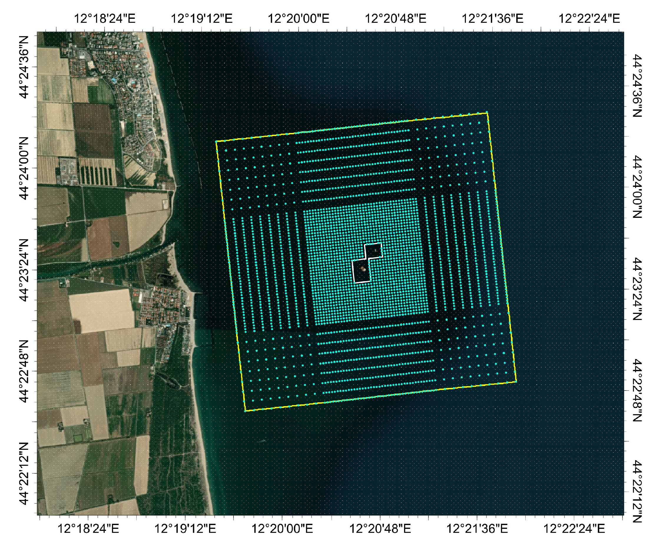
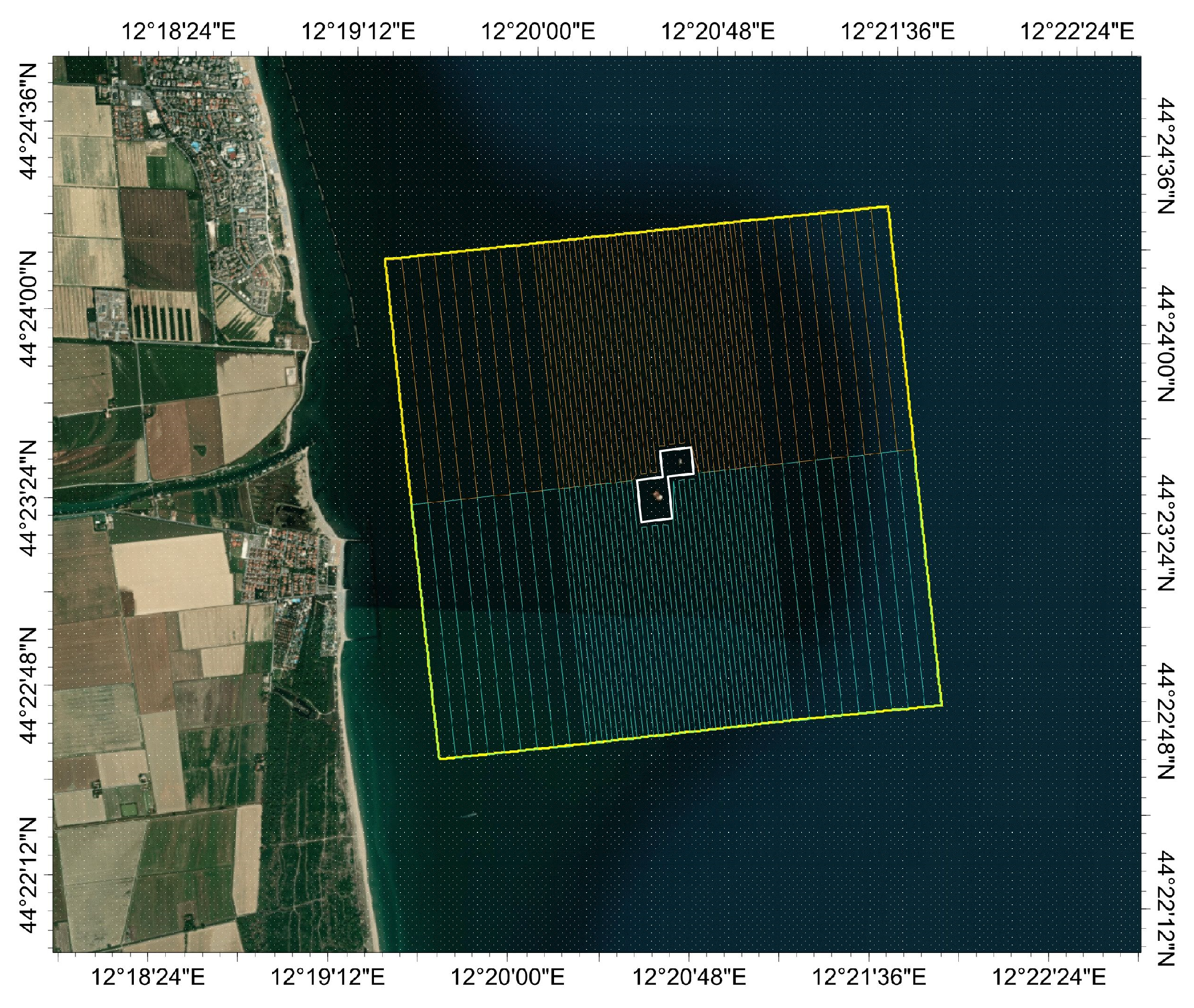
Seabed monitoring and mapping has played a relevant role in recent decades, presenting the study and implementation of increasingly advanced methodologies and technologies [28]. The decommission and reuse of existing platforms and pipelines have pushed seabed monitoring in recent years, involving large oil and gas companies in order to implement technologies and methodologies that have led to considerable scientific production and development of technology in this field [29].

Most suitable technologies for bathymetry and seabed mapping involve acoustic waves, electromagnetic waves, and visible light, with different full scales and resolutions [30].

To reconstruct the morphology of the seabed, a multibeam scanner (WBMS) with a high spatial resolution and high georeferencing was implemented. The bathymetric platform, which integrates multibeam sonar with a dedicated pressure sensor, with an optimized inertial platform and a DVL system, was equipped with an interactive network based on Least Square Support Vector Regression (LSSVR).

The LSSVR installed in the AUV control unit works synchronously with the inertial platform (IMU) and the other sensors to increase the final accuracy of the system, so that a bathymetric map can be obtained with high precision (<10 cm).

Among the possible solutions, the choice fell on a dedicated sensor that implements the MBES (Multi-Beam Eco Sounding) technology. This technique allows for the continuous acquisition of a large area, thanks to a high number of acoustic waves that are simultaneously propagated. It is possible to obtain a high spatial resolution, investigate medium-distance depth ranges, and integrate the data with a GPS signal.

According to the designed output characteristics, the most suitable instrument is the Wideband Multi-Beam Sonar (WBMS) for the high-resolution bathymetry of Norbit. The WBMS’s technical specifications are reported in

Table 1. WBMS’s technical specifications.

Technical Specifications
Range resolution	<10 mm (acoustic w. 80 kHz bandwidth)
Number of beams	256–512 EA & ED
Operating nominal frequency	400 kHz (frequency agility 200–700 kHz)
Ping rate	up to 60 Hz, adaptive
Depth range	0.2–275 m (160 m typical @400 kHz)
Resolution (across × along)	standard: 0.9O × 1.9O @400 kHz AND 0.5O × 1.0O @700 kHz.
Narrow option	0.9O × 0.9O @400 kHz and 0.5O × 0.5O @700 kHz
Depth rating	900 m
Operating temperature	−4 °C to +40 °C (topside −20 °C to +55 °C)

.

The sensor platform must have specific characteristics to obtain measurements close to the seabed, a solution conceived to increase the resolution of the detection, both in terms of depth measurement and in terms of spatial correlation. Moreover, the implementation of an autonomous survey system, operator-free, led to the development of an IoT approach, ensuring data redundancy and greater sampling frequency, and reducing costs and dangers for dive operators. So, the sensor platform was installed on board an AUV, which is an effective underwater drone, capable of navigating in total autonomy at depths of the order of 300 m below sea level. Compared to traditional bathymetry, performed with floating ships, this choice guarantees the achievement of greater spatial precision, programmed and unmanned surveys, and the possibility of conducting other types of monitoring in preparation for decommissioning [31].

The AUV chosen for this activity was the SEASTICK™ 300G AUV. This self-driving vehicle is equipped with two propeller motors called self-ring motors, which allow an operating speed of 1.2 knots, low energy consumption, and very high maneuverability.

The main feature of the AUV is the possibility of planning measurement missions, thanks to the autopilot management software, which is based on the inertial platform with ten degrees of freedom installed on board. The platform, together with other navigation tools, such as a Doppler Velocity Logger (DVL), a frontal anti-collision pinger, and a GPS, allow the drone to conduct missions autonomously, navigating along a pre-determined trajectory, maintaining a pre-established depth, and avoiding collisions with possible obstacles. The autopilot system manages all emergency systems and malfunctions to ensure vehicle integrity even in the event of breakdowns, unforeseen environmental conditions, or operator errors. A second onboard computer stores data from the sensors and synchronizes all the systems.

The system was tested in the Tyrrhenian Sea, offshore Genoa, to verify that all the components worked properly and the survey of the bathymetry of a limited area was performed. The test proved that the system performs as expected.

The main AUV technical specifications are reported in

Table 2. AUV technical specifications.

Technical Specifications
Dimensions	Length 2000 mm, diameter 140 mm
Autonomy	Up to 6 h
Max depth	300 m
Operating speed	Up to 1.2 knots
Sensors	10 degrees-of-freedom inertial platform (IMU) (piezoelectric inclinometer, three gyroscopes, three magnetometers and one barometer), integrated high-precision antenna, and GPS
Communication system	Wi-Fi 2.44 Mhz, 150 Mbps, adjustable output power, max. 27 dBm. Radius 500 m.
Additional modes	Glider, horizontal/vertical translation, and 360-degree rotation

. A full view of the AUV equipped with sensors for sea monitoring is shown in Figure 1.

3. Survey Planning

The main purpose of the survey planning phase is the definition of the optimal trajectory (nominal route) of the AUV, taking into account the characteristics of the AUV (i.e., battery duration and speed) and the environmental conditions (e.g., the direction of the sea current). The code that we developed to define the nominal route of the AUV includes the import and digitization of the georeferenced map of the area to be monitored and the setup of the survey grid in the area of interest.

To illustrate the procedure, a portion of the area located in the Adriatic Sea in front of the Ravenna coast was taken as a target example. The area is highlighted by a yellow square in Figure 2, where dedicated georeferenced maps, from the VIDEPI project of the Ministry of Economic Development of Italy [32], show the location of existing oil and gas platforms and the position of national and regional borders (referring to 2016) [33,34]. Figure 3 is an enlargement of the area of interest with a detailed view of the platforms and the definition of the boundaries of the area to be surveyed with the AUV. It lies approximately between latitudes 44°22′36″–44°22′25″ N and longitudes 12°19′21″–12°21′54″ E (WGS 84). The dimensions of the area were defined based on geomechanical analyses, which identified the rock volume potentially affected by deformations due to pressure variations and thus stress changes induced by fluid injection and/or withdrawal. The geomechanical analyses were performed with numerical models, in which the rock volume is discretized in blocks. Typically, the block size is smaller where greater variations in the parameters of interest (pressures, stresses, and deformations) occur and are larger in the peripheral zones [35]. Furthermore, the modeled rock volume is always much larger than the reservoir volume, and it extends to ground level, or the seabed if the reservoir is offshore. At the seabed level, the volume discretization corresponds to a grid. To define the optimal AUV trajectory, each cell of the grid was assigned a centroid (node), which represents a sort of virtual cornerstone that the AUV has to reach during navigation. In our example, a structured grid was used to ease the definition of a regular route (Figure 4). The nodes were then imported into the code. A polygon, representing an approximation of the buffer zone defined by the public authority for safety reasons, was defined around the platforms (grey area in Figure 3) and used to exclude the nodes within it from those considered to elaborate the nominal route of the AUV. Then, a “starting” node was selected together with the preferential direction of the AUV. The preferential direction of the AUV should coincide either with the direction of the sea current or with the direction against the current, avoiding as much as possible navigation orthogonal to the stream to minimize drift problems. The nominal route of the AUV was obtained by identifying the sequence of segments that connect all the active nodes, and the total distance to be navigated was calculated. In the example, due to the buffer zone around the platforms, the planned trajectory (Figure 5) was divided into two acquisitions to optimize the AUV route, thus reducing the duration of the survey. The navigation speed of the AUV for the planned survey was estimated by assuming the presence of a sea current with a fixed direction (i.e., North–South in the example).

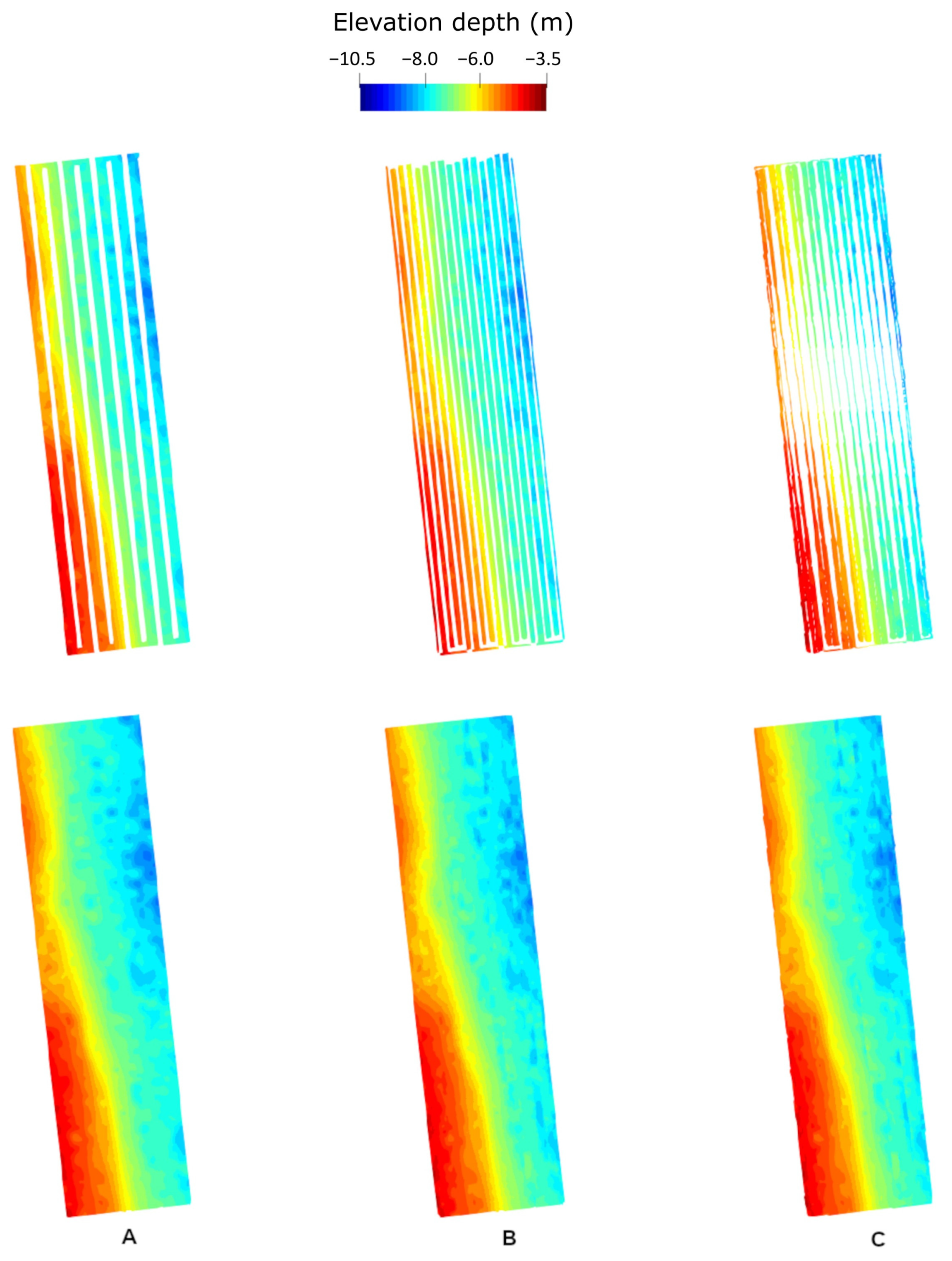
4. Seabed Mapping Based on the Measured Data

The mapping phase comprises the quality check, editing, and interpolation of the bathymetric maps.

The mapping tools typically available in commercial software dedicated to geological and geomechanical modeling offer the possibility of performing various analyses and operations on the maps, quantifying possible anomalies, and, therefore, assessing the validity of the data-acquisition process.

Following the conclusion of the AUV survey and the quality control of the bathymetric maps elaborated by the sonar tool/array, it is possible to identify three different types of criticalities that could occur due to a non-optimal acquisition: incomplete maps, overlapping maps with differences in measurements in the overlapping areas, or a combination of incomplete and overlapping maps.

These potential criticalities can be solved after the execution of the survey campaign, with the aid of proper mapping tools and procedures. As a first step, the visual analysis and accurate examination of the bathymetric surfaces with a three-dimensional viewer is essential for evaluating the quality of the elaboration and for identifying possible anomalies deriving either from the acquisition or the automatic reconstruction of the map performed by the pre-processing software installed on the AUV.

In addition to the qualitative inspection of the measured data, it is crucial to perform statistical and geostatistical analyses that support the quality control procedure by highlighting the presence of any anomalies and/or allowing a more complete examination of the final map. In particular, a full geostatistical analysis based on mean values, variance, histograms, frequency distributions, and cumulative distributions can improve the quality of the final result.

The classic variographic analysis procedure manages the data to be analyzed using different analytical models (such as the Gaussian, spherical, exponential, and ‘nugget’ models), which allow the reproduction of the trend of the bathymetry on the small–medium scale (with respect to the extension of the analyzed area), as well as calculating the tolerances on the diagnostic parameters, such as the angular tolerance with respect to the reference direction and the pitch tolerance on the distances, even with irregular bathymetric grids. A complete variographic analysis (i.e., with respect to all directions) is deemed essential to best reproduce any directional anisotropies.

To make modifications to the complete bathymetric map or portions of it based on the performed analyses, various operations can be performed, such as:

• Arithmetic operations on individual maps. They are used to make depth corrections to the original dataset measured by the sonar array. Through these operations, an alignment of different mapped sections can be obtained.
• Operations for selecting or filtering portions of maps. They can isolate specific portions of a bathymetric map to conduct selective operations. Invalid portions of the bathymetric map can be identified, eliminated, and subsequently reconstructed through interpolation techniques.
• Operations between maps. The main operations, such as union and intersection/non-intersection, allow one to perform selection operations on the portions of overlapping maps to define a final mapping based on the adopted criteria.

Different types of estimators can be employed for the reconstruction of unmapped areas or invalid portions of the surveyed area. Typical estimators employed in the reconstruction (i.e., interpolation and/or extrapolation) of topographic and bathymetric surfaces are the following: Kriging, Moving average, and Inverse Distance Weight (IDW).

In particular, Kriging is a technique used to reconstruct the trend of the bathymetric surface by integrating the variographic analysis to estimate the portions not covered by the acquisition campaign or those areas that have invalid measurements, and therefore cannot be used. Furthermore, if the seabed is characterized by a rather irregular trend, it is possible to conduct geostatistical simulations.

After the selection of the area to be monitored to assess seabed movements, a “baseline” survey must be acquired. This first survey will provide the bathymetry before any injection/withdrawal operations start and will be the reference surface for subsequent measurements during the storage lifetime. A seabed map of the area of interest, reconstructed after the geostatistical interpolation of bathymetric information, before the beginning of any type of operations, is shown in Figure 6. Since the bathymetric analysis is based on a reduced dataset with respect to the investigated area, it is necessary to apply interpolation techniques, as described previously, that can guarantee the statistical significance of the results and a solid base for comparison with subsequent measurements. Once the withdrawal/injection operations begin, the AUV will acquire new points of the seafloor level to monitor variations over time. Since the AUV measurements can be affected by uncertainties that can vary at each acquisition due to variable sea conditions and performance of the onboard equipment, the measured data must be treated so as to isolate and extract the effective bathymetric changes, eliminating or minimizing the uncertainties. In Figure 7, three different examples of bathymetric data from the AUV acquisition runs are presented, each having different characteristics (see the caption of Figure 7). The bathymetric map reconstruction is performed based on an interpolation taking into account the spatial data uncertainty and applying geostatistical techniques. The subtraction of such maps from the “baseline” bathymetric map will offer the necessary input for the validation/calibration of the geomechanical model.

5. Validation of the Geomechanical Simulations

The acquisition campaign should be periodically repeated (indicatively every 6 to 12 months depending on the underground activities) to monitor any seabed movements due to fluid storage and validate 3D geomechanical models. Geomechanical simulations were used to calculate the time and space evolution of the stresses and deformations in the reservoir, caprock, and surrounding geological formations and thus predict whether fracturing, potentially jeopardizing fluid containment, or (micro)seismicity might be triggered by underground fluid injection and withdrawal.

In addition to the definition of the differential problem and the solving method, the construction of an accurate numerical geomechanical model requires a careful description of the geological formations in terms of geometry and associated geomechanical parameters. In this perspective, the recently formalized Virtual Element Method (VEM) [36,37,38,39] represents a promising generalization of the classical conforming Finite Element Method (FEM). It only requires defining the local approximation space and carefully choosing the degrees of freedom of the elements where the solution is calculated to preserve the method’s stability and accuracy. Moreover, test and trial functions are not explicitly defined inside the elements of the discretization (thus, the name virtual elements), but it is possible to directly determine the components necessary for the evaluation of the solution [40] thanks to the definition of suitable projection operators. From these premises, it is possible to define a grid with mixed elements (general polyhedral elements) that are able to adapt to the stratigraphic structure of the investigated formations without the need to preserve conformity and guarantee a uniform cell aspect ratio. In fact, the structural mesh needs to describe the effects of sedimentation (which produces thin layers), faulting (which can cause the hydraulic connection between layers originally not in communication), or erosion (which produces degenerated layers). Based on these observations, the implemented gridding procedure reconstructs stratigraphic and faulting surfaces, if any [41], and uses them as constraints of the tetrahedrization process. The resulting unstructured grid can be refined in the zones where high accuracy is required. Then, VEM [36,37,38,39] was applied to the solution of the stress–strain equilibrium equations under the hypothesis of small deformations on large rock volumes subject to pore pressure variations. Successful validation tests were performed against a Finite Element Method (FEM) commercial software on a realistic gas storage scenario (see [42,43] for a detailed description) under the hypothesis of isotropic elastoplastic constitutive laws. However, a viscoelastic constitutive model can also be adopted depending on the scenario to be simulated.

The last step of the model construction is to provide reliable values of the relevant geomechanical parameters for each geological formation. One of the key parameters for the geomechanical characterization is the normal elastic modulus or Young’s modulus (E), which represents the stiffness of the porous medium and governs deformations and displacements. Young’s modulus is estimated both through laboratory measurements, such as those conducted with mono- and triaxial tests and with oedometer tests (“static” value, E_s), and through the analysis of the propagation of sonic waves inside the rock (“dynamic” value E_d). For this reason, an extensive study was performed to obtain representative trends of the dynamic Young’s modulus with depth for the lithologies observed in the Po Plain and the North Adriatic offshore area. From 1957 to the present, more than 2000 wells have been drilled, and hundreds of kilometers of seismic sections have been acquired. A large part of the well and seismic data was made public through a database constructed in the framework of the VIDEPI project already mentioned before. Log profiles always include the lithological analysis and the identification of hydrocarbon-bearing intervals, and often also the registration of the sonic log that is fundamental for calculating the dynamic Young’s modulus.

The available data from the well profiles were collected, digitized, and analyzed in previous works [44,45]. Benetatos et al. [44] were able to group the identified lithologies into nine lithological groups (six clastic, one marly, and two carbonatic). They applied linear regression to each one to extract the relation of sonic P-wave velocity variation with depth (Figure 8).

For the calculation of the dynamic Young’s modulus E_d, the following formula was used:

$$E_d=\frac{\rho V_S^2(3V_P^2-4V_S^2)}{V_P^2-V_S^2}$$

(1)

where V_P is the velocity of the primary waves (P-), vs. is the velocity of the secondary or shear waves (S-), and ρ is the density of the formation. While V_P was obtained directly from the sonic log readings, S-wave velocity and density were estimated separately.

In the Italian context, several studies related to the V_P/V_S ratio have been published, most of which are based on seismological surveys using local or teleseismic data. In most cases, the investigated rock volume extends for several kilometers in the subsurface. The authors of [46] studied the upper part of the crust in the Friuli area and found values in the range of 1.75–1.93 for the first 12 km of depth. The authors of [47] found a mean value of 1.79 ± 0.05 for depths down to the Moho discontinuity. Similar values (slightly higher than 1.75) were also obtained by [48], who performed a study using local data for the entire Italian peninsula and depths down to almost 60 km. For the upper part of the crust (first 1–2 km), no systematic study of the V_P/V_S ratio is available for the Italian territory. To determine the velocity of the seismic shear waves (-S) in the depth range of interest, we used a V_P/V_S ratio curve derived from the work of [49] that used seismic, sonic logs, and laboratory measurements to obtain velocity data for clastic silicate rocks. On these data, we performed a regression analysis to obtain an intermediate V_P/V_S curve that we applied to the P-wave velocity values for each of the lithological groups proposed by [44].

The obtained V_P/V_S ratio showed high values (>2) at shallow depths (less than 2 km), most likely due to poor sediment consolidation and high water saturation. The values progressively decreased with depth and the curve reached a value close to 1.75 (Figure 9).

The calculation of the rock density, which is also shown in the equation for the calculation of the dynamic Young’s modulus, was based on the formula proposed by [50] and recently adopted by [51], who studied several sonic logs in the Po Valley area:

$$\rho =d·V_p^f$$

(2)

where ρ is the density (g/cm³), V_P is the velocity of the primary seismic waves (km/s), and d and f are constants that have values of 1.75 and 0.265, respectively, based on the results obtained by [52].

The variation in the values of the dynamic Young’s modulus was used to describe the trend of the modulus versus depth for all the recognized lithologies. Figure 10 shows the results for each lithology. The values of the dynamic Young’s modulus for all lithologies show a gradual increase with depth.

The integrated monitoring process also requires the knowledge of the pore pressure variations induced by the injection/withdrawal operations. Pressure changes represent the forcing term of the geomechanical model to simulate the variation in the stress–strain state in space and time. One of the outcomes of the simulations is the seabed vertical displacement. Recalling the target example illustrated above, a possible displacement map is shown (Figure 11). Consequently, the new bathymetric map can be reconstructed (Figure 12).

6. Conclusions

We developed all the technological, planning, and modeling components of a methodology to detect the bathymetric profile of the seabed and thus assess seabed movements induced by offshore underground activities. While it is common practice to monitor ground-level through InSAR measurements, the seabed level above offshore reservoirs and storage can be subject to regular inspection using a Wideband Multi-Beam Sonar installed on an Autonomous Underwater Vehicle.

The main novelties of this methodology are:

• The integration of knowledge from different disciplines (physics, engineering, geomechanics, modeling, and ICT) to provide improved reservoir and storage monitoring;
• The implementation of a multibeam scanner with a high spatial resolution and high georeferencing, integrated with other sensors, for the detection of the bathymetry with high accuracy (<10 cm);
• The possibility to validate or calibrate geomechanical models of offshore reservoirs or storage based on periodical seabed monitoring and thus to indirectly assess safety conditions.

To illustrate and discuss our methodology, we proposed its application to a synthetic yet realistic case study in the Adriatic Sea, Italy, where several depleted gas reservoirs could be potentially converted into underground fluid storage in the near future. However, the methodology can be extended to any offshore area where underground activities are ongoing or under development.

References

1. Jeanne, P.; Zhang, Y.; Rutqvist, J. Influence of Hysteretic Stress Path Behavior on Seal Integrity during Gas Storage Operation in a Depleted Reservoir. J. Rock Mech. Geotech. Eng. 2020, 12, 886–899. [Google Scholar] [CrossRef]
2. Kumar, K.R.; Honorio, H.T.; Hajibeygi, H. Simulation of the Inelastic Deformation of Porous Reservoirs under Cyclic Loading Relevant for Underground Hydrogen Storage. Sci. Rep. 2022, 12, 21404. [Google Scholar] [CrossRef] [PubMed]
3. Huang, M.-T.; Zhai, P.-M. Achieving Paris Agreement Temperature Goals Requires Carbon Neutrality by Middle Century with Far-Reaching Transitions in the Whole Society. Adv. Clim. Chang. Res. 2021, 12, 281–286. [Google Scholar] [CrossRef]
4. Rogelj, J.; den Elzen, M.; Höhne, N.; Fransen, T.; Fekete, H.; Winkler, H.; Schaeffer, R.; Sha, F.; Riahi, K.; Meinshausen, M. Paris Agreement Climate Proposals Need a Boost to Keep Warming Well below 2 °C. Nature 2016, 534, 631–639. [Google Scholar] [CrossRef] [Green Version]
5. IEA. Net Zero by 2050—A Roadmap for the Global Energy Sector 2021. p. 224. Available online: https://iea.blob.core.windows.net/assets/063ae08a-7114-4b58-a34e-39db2112d0a2/NetZeroby2050-ARoadmapfortheGlobalEnergySector.pdf (accessed on 4 July 2023).
6. Hydrogen TCP-Task 42. In Underground Hydrogen Storage: Technology Monitor Report; TNO - Netherlands Organisation for Applied Scientific Research: Delft, The Netherlands, 2023; p. 153.
7. Bocchini, S.; Castro, C.; Cocuzza, M.; Ferrero, S.; Latini, G.; Martis, A.; Pirri, F.; Scaltrito, L.; Rocca, V.; Verga, F.; et al. The Virtuous CO2 Circle or the Three Cs: Capture, Cache, and Convert. J. Nanomater. 2017, 2017, 6594151. [Google Scholar] [CrossRef] [Green Version]
8. Benetatos, C.; Salina Borello, E.; Peter, C.; Rocca, V.; Romagnoli, R. Considerations on Energy Transition. GEAM Geoing. Ambient. E Min. 2019, 158, 26–31. [Google Scholar]
9. Benetatos, C.; Bocchini, S.; Carpignano, A.; Chiodoni, A.; Cocuzza, M.; Deangeli, C.; Eid, C.; Ferrero, D.; Gerboni, R.; Giglio, G.; et al. How Underground Systems Can Contribute to Meet the Challenges of Energy Transition. GEAM Geoing. Ambient. E Min. 2021, 58, 65–80. [Google Scholar] [CrossRef]
10. Rocca, V.; Viberti, D. Enviromental Sustainability of Oil Industry. Am. J. Environ. Sci. 2013, 9, 210–217. [Google Scholar] [CrossRef] [Green Version]
11. Verga, F. What’s Conventional and What’s Special in a Reservoir Study for Underground Gas Storage. Energies 2018, 11, 1245. [Google Scholar] [CrossRef] [Green Version]
12. Ajayi, T.; Gomes, J.S.; Bera, A. A Review of CO2 Storage in Geological Formations Emphasizing Modeling, Monitoring and Capacity Estimation Approaches. Pet. Sci. 2019, 16, 1028–1063. [Google Scholar] [CrossRef] [Green Version]
13. Aminu, M.D.; Nabavi, S.A.; Rochelle, C.A.; Manovic, V. A Review of Developments in Carbon Dioxide Storage. Appl. Energy 2017, 208, 1389–1419. [Google Scholar] [CrossRef] [Green Version]
14. Ravenna CCS. Available online: https://ccushub.ogci.com/focus_hubs/ravenna/ (accessed on 25 May 2023).
15. Matos, C.R.; Carneiro, J.F.; Silva, P.P. Overview of Large-Scale Underground Energy Storage Technologies for Integration of Renewable Energies and Criteria for Reservoir Identification. J. Energy Storage 2019, 21, 241–258. [Google Scholar] [CrossRef]
16. Pawar, R.J.; Bromhal, G.S.; Carey, J.W.; Foxall, W.; Korre, A.; Ringrose, P.S.; Tucker, O.; Watson, M.N.; White, J.A. Recent Advances in Risk Assessment and Risk Management of Geologic CO2 Storage. Int. J. Greenh. Gas Control 2015, 40, 292–311. [Google Scholar] [CrossRef] [Green Version]
17. Newell, P.; Ilgen, A.G. Overview of Geological Carbon Storage (GCS). In Science of Carbon Storage in Deep Saline Formations; Elsevier: Amsterdam, The Netherlands, 2019; pp. 1–13. ISBN 978-0-12-812752-0. [Google Scholar]
18. Zhao, K.; Jia, C.; Li, Z.; Du, X.; Wang, Y.; Li, J.; Yao, Z.; Yao, J. Recent Advances and Future Perspectives in Carbon Capture, Transportation, Utilization, and Storage (CCTUS) Technologies: A Comprehensive Review. Fuel 2023, 351, 128913. [Google Scholar] [CrossRef]
19. Orlic, B.; Wassing, B.B.T.; Geel, C.R. Field Scale Geomechanical Modeling for Prediction of Fault Stability during Underground Gas Storage Operations in a Depleted Gas Field in The Netherlands; OnePetro: Richardson, TX, USA, 2013. [Google Scholar]
20. Teatini, P.; Castelletto, N.; Ferronato, M.; Gambolati, G.; Janna, C.; Cairo, E.; Marzorati, D.; Colombo, D.; Ferretti, A.; Bagliani, A.; et al. Geomechanical Response to Seasonal Gas Storage in Depleted Reservoirs: A Case Study in the Po River Basin, Italy. J. Geophys. Res. Earth Surf. 2011, 116, JF001793. [Google Scholar] [CrossRef]
21. Tamburini, A.; Conte, S.D.; Ferretti, A.; Rucci, A. Monitoring Surface Deformation with Satellite InSAR—A Tool for Time Lapse Analysis of UGS. Geosci. Eng. 2015, 2015, 1–5. [Google Scholar]
22. Raziperchikolaee, S.; Cotter, Z.; Gupta, N. Assessing Mechanical Response of CO2 Storage into a Depleted Carbonate Reef Using a Site-Scale Geomechanical Model Calibrated with Field Tests and InSAR Monitoring Data. J. Nat. Gas Sci. Eng. 2021, 86, 103744. [Google Scholar] [CrossRef]
23. Antoncecchi, I.; Ciccone, F.; Rossi, G.; Agate, G.; Colucci, F.; Moia, F.; Manzo, M.; Lanari, R.; Bonano, M.; De Luca, C.; et al. Soil Deformation Analysis through Fluid-Dynamic Modelling and Dinsar Measurements: A Focus on Groundwater Withdrawal in the Ravenna Area (Italy). Bull. Geophys. Oceanogr. 2021, 62, 301–318. [Google Scholar] [CrossRef]
24. Hannis, S.; Chadwick, A.; Connelly, D.; Blackford, J.; Leighton, T.; Jones, D.; White, J.; White, P.; Wright, I.; Widdicomb, S.; et al. Review of Offshore CO2 Storage Monitoring: Operational and Research Experiences of Meeting Regulatory and Technical Requirements. Energy Procedia 2017, 114, 5967–5980. [Google Scholar] [CrossRef] [Green Version]
25. Hernández, J.D.; Istenic, K.; Gracias, N.; García, R.; Ridao, P.; Carreras, M. Autonomous Seabed Inspection for Environmental Monitoring. In Proceedings of the Robot 2015: Second Iberian Robotics Conference; Reis, L.P., Moreira, A.P., Lima, P.U., Montano, L., Muñoz-Martinez, V., Eds.; Springer International Publishing: Cham, Switzerland, 2016; pp. 27–39. [Google Scholar]
26. Zwolak, K.; Wigley, R.; Bohan, A.; Zarayskaya, Y.; Bazhenova, E.; Dorshow, W.; Sumiyoshi, M.; Sattiabaruth, S.; Roperez, J.; Proctor, A.; et al. The Autonomous Underwater Vehicle Integrated with the Unmanned Surface Vessel Mapping the Southern Ionian Sea. The Winning Technology Solution of the Shell Ocean Discovery XPRIZE. Remote Sens. 2020, 12, 1344. [Google Scholar] [CrossRef] [Green Version]
27. Wynn, R.B.; Huvenne, V.A.I.; Le Bas, T.P.; Murton, B.J.; Connelly, D.P.; Bett, B.J.; Ruhl, H.A.; Morris, K.J.; Peakall, J.; Parsons, D.R.; et al. Autonomous Underwater Vehicles (AUVs): Their Past, Present and Future Contributions to the Advancement of Marine Geoscience. Mar. Geol. 2014, 352, 451–468. [Google Scholar] [CrossRef] [Green Version]
28. Smith Menandro, P.; Cardoso Bastos, A. Seabed Mapping: A Brief History from Meaningful Words. Geosciences 2020, 10, 273. [Google Scholar] [CrossRef]
29. Antoncecchi, I.; Rossi, G.; Bevilacqua, M.; Cianella, R.; Vico, G.; Ferrero, S.; Catania, F.; Pacini, M.; Mondelli, N.; Rovere, M.; et al. Research Hub for an Integrated Green Energy System Reusing Sealines for H2 Storage and Transport. EEMJ 2020, 19, 1647–1656. [Google Scholar] [CrossRef]
30. Ferreira, I.O.; Andrade, L.C.d.; Teixeira, V.G.; Santos, F.C.M. State of Art of Bathymetric Surveys. Bol. Ciências Geodésicas 2022, 28, e2022002. [Google Scholar] [CrossRef]
31. Jones, D.O.B.; Gates, A.R.; Huvenne, V.A.I.; Phillips, A.B.; Bett, B.J. Autonomous Marine Environmental Monitoring: Application in Decommissioned Oil Fields. Sci. Total Environ. 2019, 668, 835–853. [Google Scholar] [CrossRef]
32. ViDEPI. Available online: https://www.videpi.com/videpi/videpi.asp (accessed on 8 May 2023).
33. ISTAT. Dataset “Confini Delle Unità Amministrative a Fini Statistici al 1° Gennaio 2023.”, Italian National Istitute of Statistics, Rome, Italy. Available online: https://www.istat.it/it/archivio/222527 (accessed on 8 May 2023).
34. Brighenti, G.; Macini, P.; Mesini, E. Subsidence Induced by Offshore Gas Production in the Northern Adriatic Sea; OnePetro: Richardson, TX, USA, 2001. [Google Scholar]
35. Suriano, A.; Peter, C.; Benetatos, C.; Verga, F. Gridding Effects on CO2 Trapping in Deep Saline Aquifers. Sustainability 2022, 14, 15049. [Google Scholar] [CrossRef]
36. Da Veiga, L.B.; Brezzi, F.; Marini, L.D.; Russo, A. Basic Principles of Virtual Element Methods. Math. Model. Methods Appl. Sci. 2013, 23, 199–214. [Google Scholar] [CrossRef]
37. Beirão da Veiga, L.; Brezzi, F.; Marini, L.D.; Russo, A. The Hitchhiker’s Guide to the Virtual Element Method. Math. Model. Methods Appl. Sci. 2014, 24, 1541–1573. [Google Scholar] [CrossRef] [Green Version]
38. Beirão da Veiga, L.; Brezzi, F.; Marini, L.D.; Russo, A. Virtual Element Implementation for General Elliptic Equations. In Building Bridges: Connections and Challenges in Modern Approaches to Numerical Partial Differential Equations; Barrenechea, G.R., Brezzi, F., Cangiani, A., Georgoulis, E.H., Eds.; Springer International Publishing: Cham, Switzerland, 2016; pp. 39–71. ISBN 978-3-319-41640-3. [Google Scholar]
39. Beirão da Veiga, L.; Dassi, F.; Russo, A. High-Order Virtual Element Method on Polyhedral Meshes. Comput. Math. Appl. 2017, 74, 1110–1122. [Google Scholar] [CrossRef]
40. Ahmad, B.; Alsaedi, A.; Brezzi, F.; Marini, L.D.; Russo, A. Equivalent Projectors for Virtual Element Methods. Comput. Math. Appl. 2013, 66, 376–391. [Google Scholar] [CrossRef]
41. Serazio, C.; Tamburini, M.; Verga, F.; Berrone, S. Geological Surface Reconstruction from 3D Point Clouds. MethodsX 2021, 2021, 101398. [Google Scholar] [CrossRef] [PubMed]
42. Benetatos, C.; Codegone, G.; Deangeli, C.; Giani, G.P.; Gotta, A.; Marzano, F.; Rocca, V.; Verga, F. Guidelines for the Study of Subsidence Triggered by Hydrocarbon Production. GEAM 2017, 152, 85–96. [Google Scholar]
43. Benlalam, N.; Serazio, C.; Rocca, V. VEM Application to Geomechanical Simulations of an Italian Adriatic Offshore Gas Storage Scenario. GEAM 2022, 165, 41–49. [Google Scholar] [CrossRef]
44. Benetatos, C.; Codegone, G.; Marzano, F.; Peter, C.; Verga, F. Calculation of Lithology-Specific p-Wave Velocity Relations from Sonic Well Logs for the Po-Plain Area and the Northern Adriatic Sea; Offshore Mediterranean Conference and Exhibition 2019, OMC 2019: Ravenna, Italy, 2019; p. 148084. [Google Scholar]
45. Livani, M.; Petracchini, L.; Benetatos, C.; Marzano, F.; Billi, A.; Carminati, E.; Doglioni, C.; Petricca, P.; Maffucci, R.; Codegone, G.; et al. Subsurface Geological and Geophysical Data from the Po Plain and the Northern Adriatic Sea (North Italy). Earth Syst. Sci. Data Discuss. 2023, 2023, 1–41. [Google Scholar] [CrossRef]
46. Gentile, G.F.; Bressan, G.; Burlini, L.; De Franco, R. Three-Dimensional VP and VP/VS Models of the Upper Crust in the Friuli Area (Northeastern Italy). Geophys. J. Int. 2000, 141, 457–478. [Google Scholar] [CrossRef] [Green Version]
47. Piana Agostinetti, N.; Amato, A. Moho Depth and Vp/Vs Ratio in Peninsular Italy from Teleseismic Receiver Functions. J. Geophys. Res. Solid Earth 2009, 114, B06303, 1–17. [Google Scholar] [CrossRef]
48. Scafidi, D.; Solarino, S.; Eva, C. P Wave Seismic Velocity and Vp/Vs Ratio beneath the Italian Peninsula from Local Earthquake Tomography. Tectonophysics 2009, 465, 1–23. [Google Scholar] [CrossRef]
49. Castagna, J.P.; Batzle, M.L.; Eastwood, R.L. Relationships between Compressional-Wave and Shear-Wave Velocities in Clastic Silicate Rocks. Geophysics 1985, 50, 571–581. [Google Scholar] [CrossRef]
50. Gardner, G.H.F.; Gardner, L.W.; Gregory, A.R. Formation velocity and density—The diagnostic basics for stratigraphic traps. Geophysics 1974, 39, 770–780. [Google Scholar] [CrossRef] [Green Version]
51. Montone, P.; Mariucci, M.T. P-Wave Velocity, Density, and Vertical Stress Magnitude Along the Crustal Po Plain (Northern Italy) from Sonic Log Drilling Data. Pure Appl. Geophys. 2015, 172, 1547–1561. [Google Scholar] [CrossRef] [Green Version]
52. Mavko, G.; Mukerji, T.; Dvorkin, J. The Rock Physics Handbook: Tools for Seismic Analysis of Porous Media, 2nd ed.; Cambridge University Press: Cambridge, UK, 2009. [Google Scholar]
Figure 1. AUV equipped with sensors for seabed monitoring and at sea during the pilot test.
Jmse 11 01387 g001
Figure 2. Location of the area of interest (yellow rectangle) with the location of the existing oil and gas platforms (red dots) in the Adriatic Sea (center of the yellow area, LAT 44°23′35″ N and LONG 12°20′40″ E WGS 84).
Jmse 11 01387 g002
Figure 3. Zoomed-in view of the Ravenna coastline and the area of interest (yellow rectangle with two platforms in the center).
Jmse 11 01387 g003
Figure 4. Filtered set of centroids of the geomechanical grid with the exclusion of the platform areas. The yellow rectangle represents the survey area, corresponding to the lateral extension of the geomechanical model.
Jmse 11 01387 g004
Figure 5. Planned trajectory of the AUV for the survey. The two sub-trajectories are represented by the orange and light-blue lines.
Jmse 11 01387 g005
Figure 6. Final realistic bathymetric map of the area of interest (UTM-33N Cartesian coordinate system) resulting from the post-processing of the acquired data (SGS realization taking into account the bathymetry variability of the decametric scale).
Jmse 11 01387 g006
Figure 7. The top images show AUV data-acquisition examples ((A) optimal acquisition (B) overlapping point acquisition, and (C) missing point acquisition) and the bottom images correspond to interpolated maps obtained from geostatistical techniques.
Jmse 11 01387 g007
Figure 8. Relations between sonic velocity and depth for each lithological group recognized from the well profiles. The black line corresponds to the simple linear regression, while the yellow rhombs indicate the average value with the corresponding standard deviation (modified figure from [44]).
Jmse 11 01387 g008
Figure 9. VP/VS ratios from shales and saturated sands from the Gulf of Mexico (dashed lines). Adopted VP/VS curve for this study (red line) (modified from [49]).
Jmse 11 01387 g009
Figure 10. Trend of the dynamic Young’s modulus for each lithology from the 1:1000 profiles available in the VIDEPI dataset.
Jmse 11 01387 g010
Figure 11. Vertical displacement map in the area of interest (UTM-33N Cartesian coordinate system) resulting from the geomechanical simulations of the rock volume, which includes the reservoir subject to injection.
Jmse 11 01387 g011
Figure 12. Bathymetry of the area of interest (UTM-33N Cartesian coordinate system) from the geomechanical simulations of the rock volume, which includes the reservoir subject to fluid injection.
Jmse 11 01387 g012