Understanding the Effects of Wind Intensity, Forward Speed, and Wave on the Propagation of Hurricane Harvey Surges

Abstract

Hurricane storm surges are influenced by wind intensity, forward speed, width and slope of the ocean bottom, central pressure, angle of approach, shape of coastal lines, local features, and storm size. A numerical experiment is conducted using the Advanced Circulation + Simulation and Simulating Waves Nearshore (ADCIRC + SWAN) coupled model for understanding the effects of wind intensity, forward speed, and wave on the storm surges caused by Hurricane Harvey. The ADCIRC + SWAN is used to simulate hurricane storm surges and waves. The wind fields of Hurricane Harvey were reconstructed from observed data, aided by a variety of methodologies and analyses conducted by Ocean Weather Inc (OWI) after the event. These reconstructed wind fields were used as the meteorological forcing in the base case in ADCIRC+SWAN to investigate the storm surges caused by the hurricane. Hurricane Harvey was the second most costly hurricane in the United States, causing severe urban flooding by dropping more than 60 inches of rainfall in Texas. The hurricane made three landfalls, with its first landfall as a Category 4 based on the Saffir–Simpson Hurricane Wind Scale (SSHWS), with wind intensities of 212.98 km/h (59 m/s). The storm surges caused by Hurricane Harvey were unique due to the slow speed, crooked tracks, triple landfalls in the USA, and excessive rain. The model’s storm surge and wave results were compared against observed data. High water marks at 21 locations and time series at 12 National Oceanic and Atmospheric Administration (NOAA) gauges were compared with the generated results. Several cases were investigated by increasing or decreasing the wind intensity or hurricane forward speed by 25% of the OWI wind and pressure data. The effects of the wave were analyzed by comparing the results obtained from ADCIRC + SWAN (with waves) and ADCIRC (without waves) models. The study found that the changes in wind intensity had the most significant effect on storm surges, followed by wave and forward speed changes. This study signifies the importance of considering these factors to enhance accuracy in predicting storm surges.

1. Introduction

A hurricane is the most destructive force formed in the deep ocean and is marked by storm winds and lower atmospheric pressures. A tropical storm is an extreme disturbance of the atmosphere in the deep ocean during the summer. According to the National Hurricane Center, the components of a hurricane include a pre-existing weather disturbance, warm tropical oceans, moisture, and relatively light winds moving upward while colder winds fall downward [1]. On an average three-year period, five hurricanes strike the United States coastline, resulting in the loss of approximately 50 to 100 people’s lives and about USD 450 billion in damage to properties from Texas to Maine [1].

Hurricane storm surges are influenced by wind intensity, forward speed, width and slope of the ocean bottom, central pressure, angle of approach, the shape of coastal lines, local features, and storm size [1,2,3,4].

A recent numerical experimental study on Hurricane Irma by Musinguzi et al. [2] analyzed the role of wind intensity, forward speed, pressure, and hurricane track on storm surges in Florida. The result from this study shows that an increase of wind intensity by 10% leads to a rise in the peak surges by 0.2 m around the landfall areas, while the same amount of surge reduction occurs when the wind intensity is reduced by 10%. A study on Hurricane Ike by Sebastian et al. [5] in Galveston Bay also found approximately 23% (+/−3%) higher water surge by increasing wind speed by 15%.

The shape of coastal lines and local features also play a role, with inward-curving coastlines experiencing more significant surges than outside-curving coastlines. For instance, surge heights are higher in Apalachee Bay in Florida than in North Carolina due to the nature of the coastal line curvature [4]. In the case of Hurricane Ike, its large wind field and concave geometry of the Louisiana–Texas coastline contributed to waves and surges that impacted over 1000 km of the coastline [6].

The approach angle is another crucial factor affecting hurricane surges, with perpendicular onshore winds causing more significant damage than parallel coast winds. The direction of the wind during Hurricane Irma, for example, caused less surge on the west coast due to near perpendicular offshore winds. However, surges returned on the west coast when the wind became onshore after the hurricane eye passed over a location.

Forward speed is also influential as the reduction of forward speed by 10% increased the peak surge of Hurricane Irma on the south side of Florida Key by more than 0.4 m while decreasing the surge by the same amount on the north side [2].

Wave contribution to storm surges has been studied as well. A study on Hurricane Irma by Musinguzi et al. [7] found that wave runup significantly impacts the total water levels on the south and northeast coasts, increasing the surge by 0.25 m in those areas. The wind blowing onshore over a long distance from the deep ocean causes water from the ocean to load onto the east coast, leading the wave to increase storm surges. The Significant Wave Height is also higher in the open ocean and deep water, regardless of the hurricane details [8].

According to the National Hurricane Center, Hurricane Harvey alone caused USD 125 billion in damage, more than any hurricane in the history of the USA, except for Hurricane Katrina [9]. It damaged over two hundred thousand houses. On 1 September 2017, one-third of Houston was underwater after 24.5 trillion gallons of water fell in southeast Texas and southern Louisiana [10]. The surges due to Hurricane Harvey were unique due to the storm’s slow speed, crooked tracks, triple landfalls, and excessive rain.

The information provided above highlights the significant impact and complexity of Hurricane Harvey, including its record-breaking damage and rainfall. Compound flooding, resulting from storm surges, river discharge, and precipitation, played a significant role in the flooding experienced during this hurricane. Different studies have examined the contributions of various factors and their interactions in generating storm surges and flooding [9,10,11,12,13,14].

A study [11] by the University of Florida and the National Oceanic and Atmospheric Administration (NOAA) states that with about 7.6 × 10¹⁰ m³ of rain over three days in Houston, Hurricane Harvey caused compound flooding. Storm surges from the ocean provided the “first punch”, the Buffalo Bayou discharge represented a “second punch”, and the San Jacinto River discharge inflicted a “third punch”. This study compared the effects of river discharge, atmospheric wind and pressure forcing, and ocean forcing on the overall surges at different stations. It is evident that the stations near the river mouth, such as Manchester and Morgan Points, are heavily influenced by the river discharge contributions. However, stations in the ocean, away from the river mouth, such as Eagle Point and Galveston Bay Entrance, had little effect of the river discharge on their surges.

The compounding factors for the extreme flooding around Galveston Bay were studied [12] by analyzing the contribution of significant forcing such as ocean, rivers, and precipitation at seven NOAA gauge stations. These stations were Manchester, Morgan Point, Eagle Point, Rollover 156 Pass, Galveston Pier, Galveston Bay Entrance, and Freeport Harbor. The compound effects are most severe at upstream stations [12]. Manchester is located deep in the river mouth and is heavily dominated by precipitation and river flows. The Galveston Bay area stations are sheltered by the Great Island and land strip. The compound effects are found to be important, and a nonlinear behavior among different factors is noticed. The downstream stations, such as Galveston Pier, Galveston Bay Entrance, and Freeport Harbors, are heavily dominated by the ocean factor as they are open to the Gulf. Coastal regions open to the ocean are flooded due to the storm surge.

A study was done on isolated and combined impacts of storm tides, river inflows, and coastal precipitation within a physical modeling framework for six historical TCs on the North Carolina coast [13]. The combined impacts of localized rainfall-runoff and riverine contributions can increase peak storm tide by up to 0.36 m in the main stem of the Cape Fear River; however, most storms result in peak increases of 0.2 m or less. The relative timing and magnitude between storm tide, coastal rainfall, and river inflows can indicate the mechanism of compound flooding likely to be observed. Specifically, the presence of high-intensity rain bands occurring in advance of the storm’s landfall can lead to river-surge compounding, while high-intensity precipitation occurring near the time of landfall leads to rainfall-surge compounding.

The Advanced Circulation Simulation (ADCIRC) [15], aided by Hydrologic Engineering Center-River Analysis System (HEC-RAS) [16] model, was used to model compound flooding on both a watershed scale and a regional scale [14]. Comparisons with actual gauge data show that adding internal flow boundary conditions into ADCIRC to account for river discharge from multiple watersheds significantly improves accuracy in predictions of water surface elevations during coastal flooding events. One of the limitations of this study is excluding short-range wave contribution. The study suggests coupling ADCIRC with Simulating Waves Nearshore (SWAN) [17] should improve the prediction [14].

The current study presents numerical experimentation on the hindcast of Hurricane Harvey storm surges and the effects of wind intensity, forward speed, and wave on storm surges using the ADCIRC + SWAN model. It follows the same procedure for Hurricane Irma mentioned earlier [2]. Every hurricane is unique in its characteristics and potential to bring in surges. Studying the effects of different storm factors on surges is vital to understand surge generation and propagation and identifying if any common behaviors among other hurricane surges exist. Currently, ADCIRC+SWAN cannot directly incorporate rain contributions in the simulation and requires the coupling of external models for it. It also cannot add river contributions unless river influx boundary conditions are incorporated in the mesh with proper resolution. The present study focused on the storm surges in coastal regions near the open ocean and bay while neglecting the explicit consideration of river mouth effects and rain-induced river flow. However, the study did include the effect of waves, which was often overlooked by previous studies. A follow-up comparative study will incorporate the precipitation and river flow effects on the storm surges during Hurricane Harvey.

2. Hurricane Harvey Synoptic History

The summary of the genesis of Hurricane Harvey in this research paper is based on the National Hurricane Center report released on 9 May 2018 [18]. A wind flown from West Africa on 12 August 2017 formed Hurricane Harvey. A tropical depression formed on 17 August in the middle northeast of Barbados. The tropical depression turned into a tropical storm after twelve hours. It moved westward, south of a western Atlantic ridge, with a peak intensity of 20.57 m/s (40 kt) on 18 August. After passing over Barbados and St. Vincent within a five-hour difference, it gradually weakened to a tropical depression on 19 August because of the increase of northerly wind shear. It dissipated into a tropical wave over the Caribbean Sea on the same day, around 1800 UTC. The remnant traveled for the next few days passing over the Yucatan Peninsula and the Bay of Campeche.

Hurricane Harvey regenerated into a tropical depression 150 n mi west away from Progresso, Mexico. It then strengthened in an environment of light shear, very warm water with mid-level moisture on 23 August 2017. It turned northward while maneuvering around the western edge of a subtropical ridge, which resulted in the track bending toward the northwest. The whole track of Hurricane Harvey is seen in Figure 1.

The storm became a hurricane on 24 August and reached category 3 at midday on 25 August, when it had already reached the middle of Texas. It intensified to category 4 on 26 August when its center made landfall on the northern end of San Jose Island about 5 n mi east of Rockport, Texas, at 0300 UTC with 59.16 m/s wind intensity and 937 mb minimum pressure. After three hours, it made a second landfall on the Texas mainland with 54.02 m/s wind intensity and a central pressure of 948 mb southeast of Refugio on the northeast coast of Copano Bay, west of Holiday Beach. It then weakened to an 18 m/s intensity for a few days. Between 26 August and 27 August, the storm made a slow loop and drifted eastward or southeastward. Although the center passed well south of the Houston Metro and Golden Triangle areas, heavy rains fell in these locations near a stationary front on Harvey’s north and east side [18]. On 28 August, the storm center returned to the sea over Matagorda Bay while its wind slightly strengthened near and north of the center. Harvey reached a final peak intensity of 23.15 m/s late on 29 August while rolling to the north-northeast due to a strengthening ridge over the western Atlantic. Harvey slowly weakened to a tropical depression on 30 August with 20.57 m/s wind intensity after making final landfall in southwestern Louisiana [18]. Then, it moved northeastward over the south of the United States while producing heavy rain and transforming into an extratropical storm by 1 September over the Tennessee Valley. On the next day, it dissipated over northern Kentucky.

3. Methodology

3.1. Mesh and Hydrodynamic Model

The Hurricane Surge On-Demand Forecasting System (HSOFS) mesh [19] is utilized in this investigation. It consists of 3,564,104 nodes and 1,813,443 elements, covering the US coast from Maine through Texas. The mesh covers the entire Gulf of Mexico and about half of the Atlantic Ocean. The mesh is displayed in Figure 2a. The mesh has an open ocean boundary, land and internal (island) boundary, and weir boundary types, as shown in Figure 2a. The average maximum node spacing along the coast is 500 m, but it decreases to approximately 150 m in coastal areas where a finer mesh is required [19]. The HSOFS is a reasonably vetted and acceptable triangular unstructured mesh for the storm surge study around the USA coasts of the Gulf of Mexico, as shown in Figure 2a. The region of interest (Figure 2a), hurricane track, and important locations (Figure 2b) are displayed in the figure. The same mesh was used in our previous study of Hurricane Irma storm surges [2].

The ADCIRC + SWAN is the hydrodynamic coupled model used for the Hurricane Harvey storm surge hindcast. ADCIRC is a sophisticated computer program developed for studying fluid on the rotating earth. ADCIRC runs as both 2D and 3D models on both spherical and cartesian coordinates. The present study uses the spherical coordinate system.

Shallow water equations (SWEs) are used to model the hydrodynamic behavior of free surface flow, such as oceans, coastal areas, estuaries, lakes, and impoundments [20]. The SWEs are derived by depth-averaging the Reynolds equations for a column of fluid with mass and momentum conservations. In SWEs, it is assumed that vertical motions are negligible and that pressure is hydrostatic. The horizontal plane’s dimensions are far more significant than the vertical dimension. A modified version of the SWEs is used in ADCIRC. To suppress the spurious oscillations inherent to the primitive equations without dampening the solution either numerically or artificially, the Generalized Wave Continuity Equation (GWCE) [15] is used instead of the primitive continuity equation. ADCIRC solves the vertically integrated momentum equations to determine the depth-averaged velocity in two horizontal directions. The conservation equations used in ADCIRC include acceleration, wind stress, atmospheric pressure, earth–moon gravitational effects, the Coriolis force due to planetary rotation, friction drags at the sea bottom, lateral mixing, waves that ride the circulation, and other potential parameters. One must mathematically formulate the physical phenomena accurately and solve the resulting equations numerically with efficient algorithms. These equations are formulated using the traditional hydrostatic pressure and Boussinesq approximations and have been discretized in space using the finite element (FE) method and in time using the finite difference (FD) method. In Luettich et al. [15], the derivation and detailed information of these equations are presented.

Initial and boundary conditions must be known for accurate solutions to hurricane storm surges. In the present study, the model was run for 53.5 days with tidal conditions only since the tide takes a relatively long time to reach equilibrium. The resultant water elevation and velocity were then used as the initial conditions for processing the Hurricane Harvey surge simulation with OWI wind data as a time-dependent meteorological-forcing, tidal input, bottom friction, nodal attributes, Coriolis force, etc. Tidal forcing is applied at the open boundary in the deep Atlantic Ocean. The time-varying tidal condition should propagate from the open ocean to inside the domain. Zero-flux boundary conditions are applied on the land and internal boundaries. The weir boundary behaves like the land boundary if the water level is less than the weir height. If the water level is greater than the weir height at a given node, then the water overtops from the node to its paired node on the other side of the weir. The weir boundary condition must satisfy the flux balance in a local and global sense, of course. The model output included time-dependent water elevation and velocity, maximum water elevation, significant wave height, average wave period, etc.

SWAN, a wave model, is used to create short-crested wind-generated waves on top of the storm surge. The wind fields, input parameters, as well as water elevations and velocities calculated in the ADCIRC model passed to the SWAN model, which solves the wave action balance equation to calculate wave parameters, such as significant wave height and wave period, by integrating a 2D wave energy spectrum into the frequency and direction domain. The details of the wave action balance equation and other mathematical details can be found in the SWAN technical guide [17]. The wind drags formulation of Powell is included in this study, as was done in our previous studies [2,3,7]. Manning’s n bottom friction, based on the Coastal Change Analysis Program (CCAP) regional land cover data, is incorporated into ADCIRC and SWAN to represent bottom roughness.

SWAN utilizes the same HSOFS mesh as ADCIRC for the meteorological, bottom friction, water level, and current. The Manning’s n values from ADCIRC are converted to roughness lengths and applied in SWAN [17]. The Komen formulation is used to account for white capping; dissipation by depth-induced breaking and bottom friction is considered. Additionally, three wave–wave interactions (triads) are activated in the model.

The combination of ADCIRC and SWAN, referred to as ADCIRC + SWAN, allows for the prediction of reasonably accurate hurricane storm surges, including the wave effects. Note that no grid-independence analysis was performed in the present study due to a lack of resources. However, the mesh used in the present study is vetted, as already mentioned.

3.2. Meteorological Forcing

ADCIRC uses meteorological input files containing time-dependent wind velocity and atmospheric pressure fields. The wind speed is increased or decreased during the ADCIRC + SWAN run by appropriate multipliers in the control parameter input file. The forward speed adjustment requires the entire wind field to be modified in a preprocessing step. Many other control parameters and boundary condition values are read and used from ADCIRC input files.

Wind fields are reconstructed by Ocean Weather Inc (OWI) [21,22,23] using observed data and computer models after the hurricane passes. The OWI wind data are considered reliable and accurate but are only available weeks after an event [2,3]. OWI utilizes the Interactive Objective Kinematics Analysis (IOKA), a data-assimilated wind model for meteorological forcing. This model generates wind and surface pressure from observations of anemometers, land-based Doppler radar, microwave, radiometers, buoy, airborne, aircraft, coastal stations, and satellite measurements. This study uses OWI as a reference for meteorological forcing.

Various cases are modeled by varying major hurricane parameters: (1) wind intensity and (2) forward speed.

Table 1. Variable combinations used for different cases.

Case	Wind Intensity	Forward Speed
1 (Base Case)	100% (maximum 59 m/s)	100%
2	125% (maximum 73.75 m/s)	100%
3	75% (maximum 44.25 m/s)	100%
4	100% (maximum 59 m/s)	125%
5	100% (maximum 59 m/s)	75%
6 *	100% (maximum 59 m/s)	100%

* Used ADCIRC (without wave), unlike Cases 1–5 that used ADCIRC + SWAN model.

summarizes the experimental case study. Case 1 represents the base simulation in which OWI wind field data’s original values (i.e., 100% wind intensity, 100% forward speed) are maintained. Wind intensity and forward speed are increased or decreased by 25%. The higher percentage is determined with the intention to cap the maximum wind strength no higher than that of a category 5 hurricane. Case 1 was compared with observed data to examine the performance of the ADCIRC+SWAN model, while the rest of the cases were used to study the influence of each parameter on storm surge. Wind intensity signifies the strength of the hurricane’s wind field, which is time and space dependent. Forward speed is the travel speed of the hurricane’s eye, which is time-dependent.

3.3. Model Validation

The relationship between the modeled and observed water levels is measured by using the Coefficient of Determination (R²), Mean Normalized Bias (B_MN), and Root Mean Square Error (E_RMS). The R² indicates how well a data set aligns on a line with an ideal value of one. The B_MN represents the magnitude of prediction compared to the observed value with an ideal value of zero. It is calculated as follows:

$$B_{MN}=\frac{\frac{1}{N}{\sum }_{i=1}^N{E}_i}{\frac{1}{N}{\sum }_i^N\left|O_i\right|}$$

(1)

E_RMS quantifies the magnitude of an error with an ideal value of zero. It is obtained from the following equation:

$$E_{RMS}=\frac{1}{N}\sum _{i=1}^N{E}_{i^2}$$

(2)

where O is the observed value, E is the error in terms of simulated minus observed, and N is the number of data points.

The above statistics were used to demonstrate the model performance by the wet-only method with locations wetted by ADCIRC + SWAN. A total of 45 HWMs points are distributed over the Texas coast.

4. Results

4.1. Maximum Winds and Water Elevations

As the counterclockwise wind pushes the ocean water above the land on the east side of the track, higher surges are expected to be on the east than on the west. For Case 1, the maximum wind intensity is above 40 m/s around the hurricane track line, and the maximum water elevation is above 1 m, mainly on the east side of the landfall area, as seen in Figure 3a,b. For Case 2, the maximum wind intensity is increased to 50 m/s. A significantly larger domain around the east side of the track from the Texas to Mississippi coasts has a maximum water elevation higher than 1.5 m, as seen in Figure 3c,d.

For Case 3, the maximum wind intensity went down to 35 m/s, and the maximum water elevation of 1 m has restricted only to the landfall area. Higher wind intensity means a stronger overland water push by the onshore wind on the east side of a hurricane. Similar effects of wind intensity of surges were observed in previous studies of Hurricane Irma and Hurricane Rita [2,3].

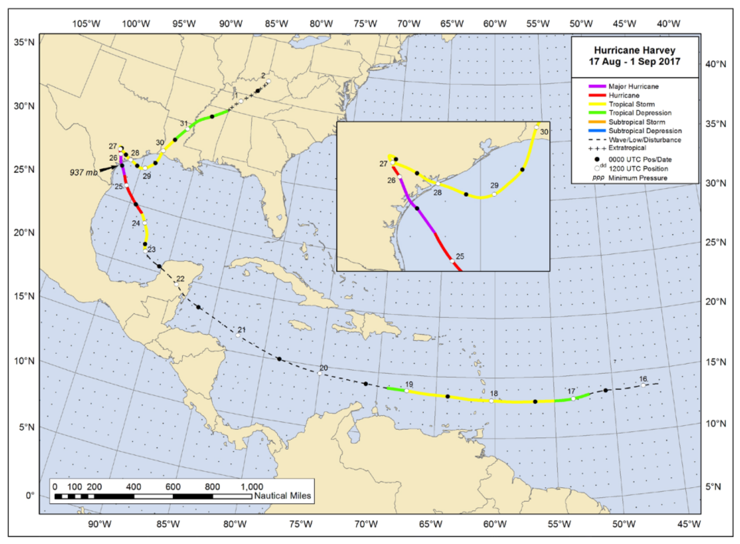
In Figure 4, wind velocity vectors at the time of landfall for Cases 1, 2, and 3 are used to demonstrate further how wind velocity directions may impact storm surges. As shown in Figure 1, Hurricane Harvey made landfall on 26 August at 0300 UTC when its center reached the northern end of San Jose Island, about 8 km northeast of Rockport, Texas [18]. On the same day, after three hours at 0600 UTC, Harvey made a second landfall on the southeast of Refugio on the northeast coast of Copano Bay, west of Holiday Beach [18]. Figure 4a–c show the first landfall, while Figure 4d–f show the second landfall with different wind intensities. The strength of Harvey was more significant at the first landfall around Rockport than the second landfall around Copano Bay due to the land interactions in between. The arrows show the asymmetric and anticlockwise wind direction of the hurricane. The storm pushed the water up on the coast from the ocean to the east side of the hurricane, toward southeastern Texas, such as Seadrift, San Antonio Bay, the Freeport, Victoria, Galveston, and so on. This explains the high-water elevation of the east side of the hurricane, as seen in Figure 3.

4.2. Qualitative Effects of Different Parameters on Maximum Water Elevations

4.2.1. Wind Intensity

The individual effect of different parameters on the maximum water elevation is illustrated by subtracting the maximum water elevations of Cases 2–5 from that of Case 1. The results are shown in Figure 5. As seen from Figure 5a, increasing the wind intensity to 125% (Case 2) increased the surge by more than 0.4 m near the landfall area around San Antonio Bay and Seadrift and by more than 0.2 m in the entire southeastern coast of Texas around Galveston, Freeport, and Trinity Bay, as shown in Figure 5a,b. About 0.2 m surge increase is visible around Corpus Christi Bay and the Louisiana coast. In southwestern Texas, the surge increased by more than 0.1 m around Padre Island. As the wind intensity decreases to 75% (Case 3), an opposite surge effect is evident, but to a lesser extent and limited along the coastline, as seen in Figure 5b.

4.2.2. Forward Speed

Increasing the forward speed to 125% barely increased the surge in an open ocean, as seen in Figure 6a. At times Harvey advanced just 5 mph, significantly less than the average hurricane forward speed of 15~19 mph. So, increasing the forward speed by 25% did not significantly impact the surges. Similar findings are reported in the study of Hurricane Irma [2]. Reducing the forward speed to 75% decreased the surge by more than 0.2 m near the landfall areas around San Antonio, as seen in Figure 6b. However, the storm surge increased by 0.4 m in southwest Texas, near Corpus Christi and Padre Island, most likely displacing water from the landfall area slide to the southwest. Interesting alternating high and low surge patches are visible in the open ocean. A slow forward-speed hurricane has enough time to push up water in the shallow coastal region, and the water level goes up by 0.1 m. Studying Hurricane Irma storm surges near Tampa Bay, Florida, also demonstrated that in smaller bodies of water, such as closed or semi-enclosed bays, slow hurricanes resulted in a more significant storm surge in the bay because of the time it takes to redistribute the mass of water [24,25].

4.3. Water Level Timeseries for Observed and Model Predictions

The water level time series of Hurricane Harvey are compared with the observed water level at 12 locations in Texas. The identification number for the NOAA gauge stations and location bathymetric depths are presented in

Table 2. National Oceanic and Atmospheric Administration (NOAA) observation stations used in the study.

	NOAA ID	Lon	Lat	Bathymetry (m)	Name
1	8775870	−97.2167	27.5800	−3.02	Bob Hall Pier, TX, USA
2	8775296	−97.3900	27.8117	−10.46	USS Lexington, Corpus Christi Bay, TX, USA
3	8775241	−97.0383	27.8367	−10.23	Aransas, Aransas Pass, TX, USA
4	8775237	−97.0733	27.8405	−12.05	Port Aransas, TX, USA
5	8774770	−97.0461	28.0216	−2.35	Rockport, TX, USA
6	8774230	−96.7945	28.2221	−0.87	Aransas Wildlife Refuge, TX, USA
7	8773037	−96.7131	28.4022	−0.76	Seadrift, TX, USA
8	8773701	−96.3950	28.4467	−3.11	Port O’Connor, TX, USA
9	8772471	−95.2950	28.9350	−9.49	Freeport SPIP, Freeport Harbor, TX, USA
10	8771341	−94.7245	29.3542	−10.25	Galveston Bay Entrance, North Jetty, TX, USA
11	8770822	−93.8417	29.69	−5.3009	Texas Point, Sabine Pass, TX, USA
12	8768094	−93.3433	29.7683	−5.9747	Calcasieu Pass, LA, USA

. The stations are displayed on the map in Figure 7a,b, and the stations, track, and wind vector snapshot at first landfall are shown in Figure 7c.

The time series of water elevation for Hurricane Harvey in Case 1 and the observed data are displayed in red and black in Figure 8(a1–a12), respectively. Additionally, the time series for different parametric cases are shown in Figure 8(b1–b12). It is observed that the surges predicted by the model are generally underpredicted at most stations. A brief discussion of each station is given below. Please refer to Figure 7a,b for each station’s geographical location and surroundings.

Bob Hall Pier is located on the left of the Hurricane Harvey track, on the east side of Padre Island, facing the Gulf of Mexico (see Figure 7a). As shown in Figure 8(a1), the time series for modeled storm surge closely matches the observed one, with some underpredictions between 0 m and 0.4 m. The surge at Bob Hall Pier is influenced by easterly and north-easterly hurricane winds pushing the water against the island, and the maximum surge recorded and modeled by Case 1 are about 1.3 m and 0.9 m, respectively. The tide frequency matches the observed data very well.

Corpus Christi station is situated by the mainland, in the inner part of Corpus Christi Bay, and is sheltered by Mustang Island. It experienced a lesser surge elevation and, in some instances, even a negative surge compared to neighboring stations such as Bob Hall Pier, which are located closer to the open ocean. The observed peak surge is about 0.4 m at Corpus Christie. Due to offshore winds on the west side of Hurricane Harvey, relatively mild flooding occurred in Corpus Christi Bay [18]. Figure 8(a2) shows that the modeled storm surge time series matches the observed data with some overprediction between 0 m and 0.12 m. A receding pattern was observed once the hurricane made landfall due to westerly wind from the land to the ocean. To the west of the landfall location, the surge decreases with distance from the landfall, resulting from the competition between counterclockwise offshore winds and the storm’s forward motion [2,5,25]. The tide frequency matches reasonably well with the observed data.

Aransas Pass, located northeast of Corpus Christie Bay, is open to the Gulf of Mexico. It experienced a similar surge as the Bob Hall Pier, but the sensor was not operational during the peak surge time, as depicted in Figure 8(a3). Aransas Pass was very close to the center (eye) of Hurricane Harvey, which could have damaged the gauge and resulted in the absence of data during the peak surge [26]. The surge peak modeled by Case 1 is approximately 1.2 m.

Port Aransas is situated near Aransas Pass but is slightly inland, sheltered by Mustang Island and San Jose Island. As a hurricane circulates counterclockwise, water is carried on from the ocean to the west of the hurricane, where the station is located (see Figure 7). Figure 8(a4) shows that the observed peak surge is 1.75 m, while Case 1 underpredicted the surge by 0.5 m. A significant surge was anticipated at Port Aransas as it was along the track’s path just before the initial landfall. A study on Hurricane Ike’s storm surges also showed the highest peak near the landfall location, as it experienced strong winds during and shortly after landfall [6]. The tide frequency matches well with the observed data.

Rockport is in the west of Aransas Bay, sheltered by San Jose Island from the Gulf of Mexico, the mainland to the west, and Aransas National Wildlife Refuge on the north. As shown in Figure 8(a5), Rockport experienced negative and positive surges due to the change of wind direction as the hurricane moved towards small islands and bay pockets. The Rockport station was very close to the center (eye) of Hurricane Harvey; this could have damaged the gauge and resulted in no data after midday of 26 August [26]. The surge predicted by Case 1 underpredicts the observed surge by about 0.2 m.

The Aransas National Wildlife Refuge is in the west of Espiritu Santo Bay, sheltered by Matagorda Island from the Gulf of Mexico. The peak surge for this station increases monotonously and then decreases afterward. The peak surge modeled by Case 1 underpredicts the observed peak by about 0.5 m and subsequently underpredicts the surge for about two days.

Seadrift is surrounded by San Antonio Bay from the west and by land from the north and east. Initially, during the incoming hurricane, a negative surge was observed until the wind started pushing from the west to raise the surge peak to approximately 1.75 m. Seadrift was located east of the hurricane, very close to the center during the first landfall, which is why it had the highest peak. The surge remained strong for two days when the hurricane hovered over Houston. Case 1 showed a similar pattern of the surges, albeit underpredicted by about 0.4 m.

Port O’Connor is open to Matagorda Bay from the north and east and is loosely sheltered by the narrow strip of Towns Island from the Gulf of Mexico. The station experienced a peak surge of approximately 1 m, and Case 1 underpredicted the peak by about 0.3 m. This station consistently gets wind from the waterside and experiences elevated surges for about five days.

Freeport is by the Gulf of Mexico, open to the ocean. It has a peak surge of about 1 m. The surges remained elevated for five days due to wind from the ocean. The surge predicted by Case 1 is similar to those observed but underpredicted by about 0.3 m.

Galveston Bay Entrance connects Galveston Bay with the Gulf of Mexico. The station is open to the Gulf of Mexico and susceptible to a hurricane’s direct hit. The surging water can move north and west through the connecting passage between the bay and the ocean. The peak surge reached approximately 1 m and remained elevated at around 0.75 m for about five days. Case 1 underpredicted the surge by about 0.25 m.

Texas Point, Sabine Pass is open to the Gulf of Mexico from the east and southeast. It is sheltered by land from the north and west. When the wind came from the ocean during the early part of the hurricane, a moderate surge of 0.5 m is visible in Figure 8(a11). A zero or negative surge was observed when the wind was predominantly from the south. Interestingly, contrary to the observed data, Case 1 shows a different tidal pattern, suggesting that the bathymetry resolution used in the model is not accurate in that location.

Calcasieu Pass is west of the Louisiana–Texas border in Cameron, Louisiana. It is open to the Gulf from the south and sheltered from the north. Calcasieu Pass experienced a consistent surge of about 0.5~0.75 m throughout Hurricane Harvey until the hurricane approached its vicinity, causing the surge to rise above 1 m, as shown in Figure 8(a12). Case 1 underpredicted the surge by about 0.25 m.

The discrepancies between model results and observed data can be attributed to various factors such as wind and pressure data, bathymetry, and mesh inaccuracies [2,3,27]. The significant errors resulting from insufficient grid resolution are primarily attributed to the misrepresentation of large velocity gradients caused by the irregular coastline [27]. The choice of model parameters, including bottom frictions and wind drag coefficients, could also contribute to the discrepancies. The exclusion of rain and river flows in the current study may have further contributed to the observed discrepancies.

4.4. Effects of Wind Intensity and Forward Speed

The effects of wind intensity and forward speed on storm surges are important factors to consider in analyzing the impacts of hurricanes. The time series of water elevation for the rest of the cases are displayed in Figure 8(b1–b12). In the case of increasing wind intensity by 25%, the surges increase consistently. The most significant impact of higher wind intensity is observed at Freeport Harbor, Entrance Galveston Bay, and Seadrift. These areas, particularly around the first landfall and on the east side of the hurricane, experience a substantial increase in surges. However, even with higher wind intensity, the surges are still underpredicted to some extent at stations like Bob Hall Pier, Port Aransas, Rockport, Aransas Wildlife Refuge, and Port O’Connor.

On the other hand, higher-intensity winds accurately predicted the surge at Seadrift, Freeport Harbor, Galveston Bay Entrance, and Calcasieu Pass. Over-prediction of the surge occurred with high wind intensity in Corpus Christi and Texas Point, Sabine Pass. Interestingly, the surge sometimes recedes due to the high wind intensity case at all stations. When higher-intensity winds blow onshore (from the ocean to the land), they increase the surge. Conversely, when the winds blow Offshore (from the land to the ocean), they recede the surge by pushing the water away from the station. Lower-intensity winds have the opposite effects on surge behavior.

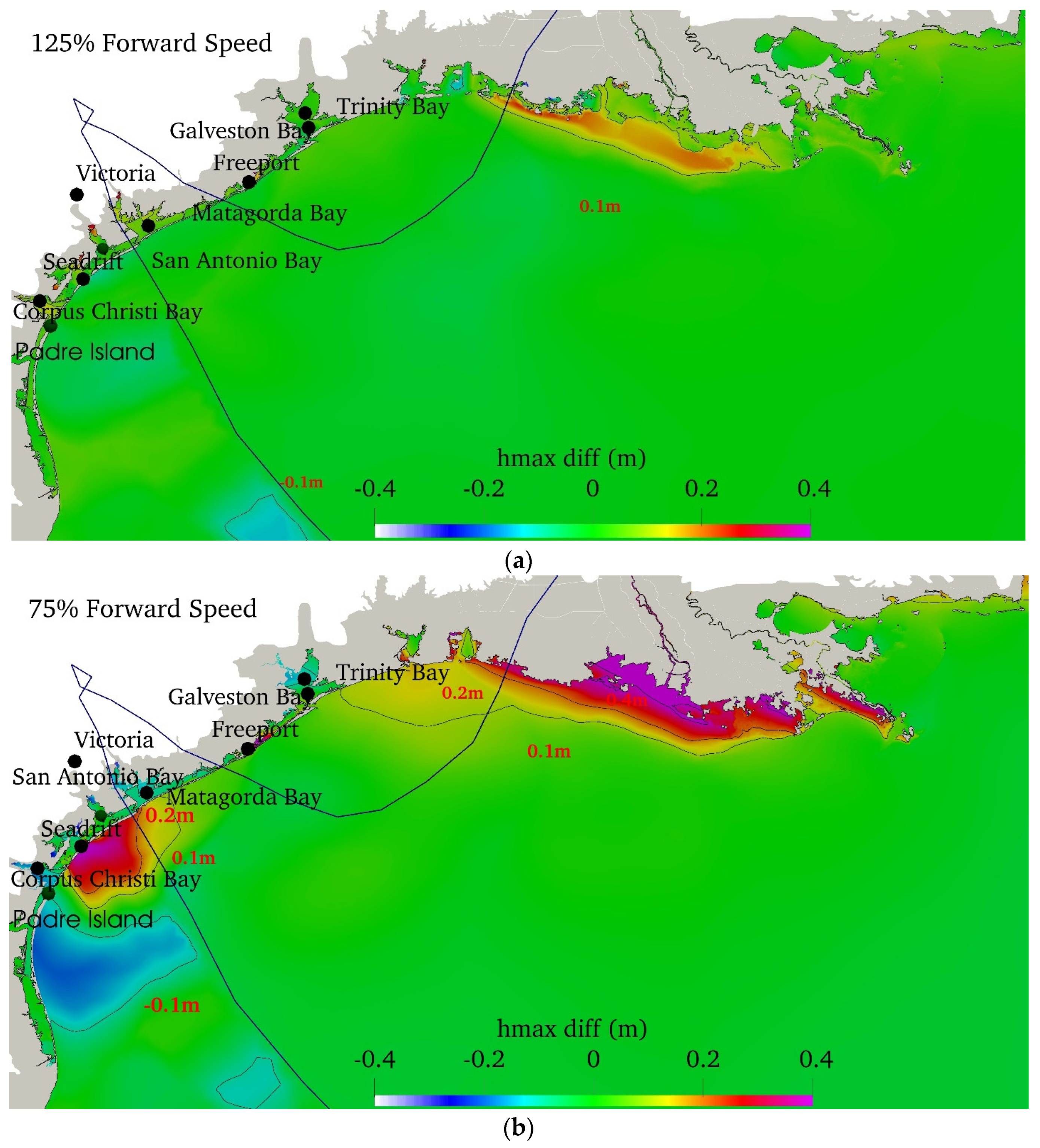
Regarding the hurricane’s forward speed, a higher forward speed brings surges faster, and the peak is advanced from about 12 to 18 h. Conversely, slower forward speed delays the surge peak from about 18 to 30 h. A previous study on Hurricane Rita by Musinguzi et al. [3] observed a phase lead of 36 h when forward speed was increased by 25%. Notably, at Corpus Christie and Port O’Connor stations, reducing forward speed had a more significant impact than increasing forward speed. This suggests that a slower hurricane gives some time for water to accumulate in the shallow estuaries while a fast-moving hurricane quickly passes over the region. The study on Hurricane Rita also found that increasing the storm’s forward speed reduces flooded volumes but increases peak surges by about 40% [3]. These observations highlight the complex relationship between hurricane forward speed and storm surge characteristics.

4.5. High-Water Marks

High water marks (HWMs) left on structures and trees after hurricane storm surges dissipate provide valuable data for evaluating the performance of the ADCIRC + SWAN model. However, in the ADCIRC + SWAN domain, some HWMs locations remained dry for various reasons, such as lack of model mesh resolution, outdated bathymetry, or inaccurate input parameters [2,27]. Therefore, only the wet stations are considered for comparison with the observed HWMs.

Figure 9 displays the comparison between model HWMs and the observed data. The model HWMs are subtracted from the observed data, and a color-coded scheme is used to indicate the accuracy of the model predictions. Purple points represent well-predicted HWMs; the surge differences are within ±0.5 m. On the other hand, the dark-purple points indicate stations with surge differences of around ±1 m or higher, suggesting more significant discrepancies between the modeled and observed HWMs.

Figure 10, the scatter plots are used to visualize the comparison between the modeled and observed HWMs. These plots quantitatively assess the model’s performance in predicting the HWMs. The scatter plots help identify the extent of agreement or disagreement between the modeled and observed data points.

These visualizations and comparisons of the modeled and observed HWMs are crucial for evaluating the accuracy and reliability of the ADCIRC + SWAN model in capturing the storm surge impacts during Hurricane Harvey. They highlight areas where the model performs well (seven purple points) and areas where improvements are needed (dark-purple points) in predicting the HWMs.

In Figure 10, the 45-degree red line is the parity line between the observed and modeled HWMs, as shown in Figure 10. It serves as a reference for comparing the two datasets. The scatter plots also display the coefficient of determinations (R²) and straight-line equations to quantify the relationship between the observed and modeled HWMs.

Based on the statistical analysis presented in

Table 3. High-water mark statistic results.

Case	R2	ERMS	BMN	Dry Points	Wet Points
Case 1 (100% Wind)	0.6118	0.179	−0.337	24	21
Case 2 (125% Wind)	0.6923	0.070	−0.065	24	21
Case 3 (75% Wind)	0.6221	0.374	−0.503	25	20
Case 4 (125% Forward Speed)	0.5676	0.205	−0.362	24	21
Case 5 (75% Forward Speed)	0.6365	0.213	−0.370	25	20

, Case 1 has an R² value of 0.6118, indicating a moderate correlation between the observed and modeled HWMs. The Mean Normalized Bias (B_MN) value of −0.337 indicates an overall underprediction by the model, and the Root Mean Square Error (E_RMS) is 0.17, suggesting an average deviation of the modeled HWMs from the observed data. It is worth noting that these statistical numbers and the quality of comparison between the model and observed data are considered reasonable based on previous studies [2,3,27].

Comparing the different cases, Case 2 improved the HWMs comparison by decreasing the ERMS to 0.07. On the other hand, Case 3 increases the ERMS to 0.374, indicating more significant discrepancies between the observed and modeled HWMs.

Regarding the forward speed, Case 4 performed slightly better than Case 5 in terms of error, although both have higher E_RMS values than Case 1.

These findings are consistent with previous studies on other hurricanes, such as Hurricane Irma [2].

4.6. Wave Effects

In this study, the contribution of waves to the rise of ocean water levels during a hurricane is examined in addition to storm surge and tide. Waves increase ocean water rise through wave runup and wave setup [7]. Wave runup occurs when waves break and propel water onto beaches, while wave setup happens when wave runup accumulates and has nowhere to go but onto the land. The hurricane storm surge is simulated in Case 6 using ADCIRC without considering any wave effects.

The time series of a hurricane storm surge at 12 stations are shown in Figure 8 in the light-green line. From the comparison between the red (Case 1—with the wave) and light-green (Case 6—without wave) lines, it is evident that wave effects almost always increased the surge in the order of centimeters. However, the wave contribution to the surge varied and reached up to 0.2~0.3 m in most stations. The difference is pronounced during the peak hurricane duration. Compared with observed data, ADCIRC + SWAN and ADCIRC slightly underpredict the surge in all stations except for Corpus Christie and Texas Point, Sabine Pass, where the models overpredicted surges.

The wave results from ADCIRC + SWAN are compared against the NOAA tidal gauge station and buoy data.

Table 4. NOAA tidal buoy stations used in the study.

Station	Lon	Lat	Bathymetry (m)	Obs/Case 1	SWH Peaks (m)	AWP Peaks (s)
42002	−93.646	26.055	−2737.9	Observed	4.79	7.31
						6.97
				Case 1	4.58	8.29
						7.36
42019	−95.345	27.910	−83.2	Observed	7.08	8.3
				Case 1	6.73	10.45
42020	−96.6	26.968N	−102.4	Observed	7.54	9.27
				Case 1	8.9	11.05
42035	−94.413	29.232	−15.8	Observed	3.58	6.16
						6.50
				Case 1	3.19	8.23
						6.82

provides information about the NOAA tidal buoy stations used in the study, including their coordinates, bathymetry, and observed Significant Wave Height (SWH) and Average Wave Period (AWP) peaks, as well as case-simulated SWH and AWP peaks.

The analysis of the simulated wave focuses on comparing SWH and AWP three hours before the first landfall, during the first landfall, and during the second landfall. Table 4 provides a summary of the observed SWH and AWP peaks, as well as the corresponding values for Case 1.

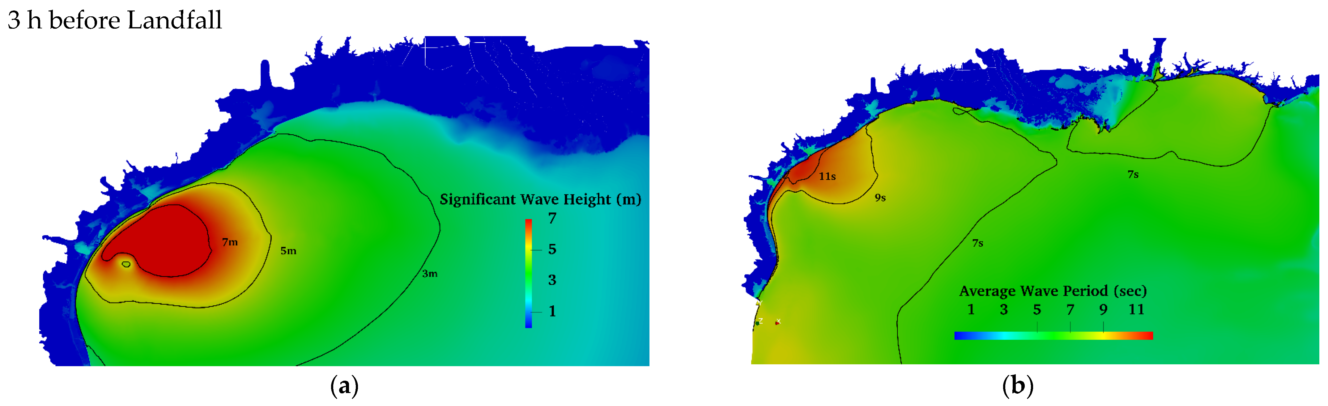
In Figure 11, the first column (i.e., Figure 11a,c,e) demonstrates the SWH and the second column (i.e., Figure 11b,d,f) shows AWP. Before and during the first landfall, the SWH exceeded 7 m due to the long fetch of the Gulf of Mexico. The entire coastal area around the landfall experiences significant SWH due to uninterrupted fetch. Similar observations were made for Florida’s east coast during Hurricane Irma [7]. During the second landfall, the SWH is around 6 m, slightly lower than the first landfall SWH. This decrease in SWH could be attributed to the fact that the hurricane weakened and slowed down as it moved back from the land to the ocean. Toward the southeast of Texas, an SWH of 3 m is observed, and the SWH decreases as it approaches land. The AWP is 11 s before and during the first landfall but decreases to 9 s before reaching Galveston during the second landfall. A higher AWP means higher energy in the swell and a larger wave.

The modeled SWH and AWP are compared with the buoy data at four stations. The locations of the stations are shown on the map in Figure 12a. The comparisons between SWH and AWP for these stations are shown in Figure 12b–e. The results suggest that ADCIRC + SWAN accurately predicts the SWH for the stations, although some of the frequency details may be lost in the modeling process.

It is observed that the peak height is overpredicted by approximately 1.8 m for buoy station 42020. This discrepancy indicates that SHW generally increases with greater water depth, a finding that aligns with previous studies [7,8]. As the waves approach the shallow water and coast, the SWH decreases. Stations 42020 and 42019, which have water depths close to 100 m and are situated near the hurricane path, exhibit SWH values close to 7 m. Station 4203, although near the hurricane’s path, is located near the coast in shallow water with a depth of 15.81 m resulting in an SWH of around 3.5 m. Station 42002, which is farther away from the hurricane’s path but in a deep ocean depth of 2727.9 m, shows a high peak SWH of nearly 5 m. These findings corroborate a previous study on Hurricane Irma, which concluded that SWH increases with ocean depth [7]. Shallow water generally exhibits shorter SWH compared to deep water. A study on hurricanes on the Hawaiian island also supports this finding, indicating that open ocean and deep water experience greater SWH regardless of the specific detail of the hurricane [8]. The station closest to the coastal region has the lowest SWH and AWP values.

The Simulated AWP profiles show a good match with the observed ones. However, the modeled AWP starts lower than the observed values, likely because the SWAN starts from scratch and takes a day or two for the wave to develop fully. Near the peak, the modeled AWP consistently overpredicts by about 2 s for all stations. The AWP peaks coincide with the SWH peaks, indicating that higher AWP values correspond to greater energy in the swell and a larger wave.

Stations 42019 and 42020, which are close to the hurricane’s path and have relatively deep water, exhibit AWP values exceeding 10 s. In the deep ocean but away from the hurricane’s path, station 42002 shows AWP peaks at around 7.5 s. In the shallow water along the hurricane’s path, station 42035 has an AWP peak of around 6 s.

These findings emphasize the importance of considering wave effects, such as AWP and surge amplification, and accurately modeling and predicting hurricane impacts, particularly in coastal regions with complex coastlines. Overall, these results provide valuable insights into the relationship between ocean depth, SWH, and AWP, highlighting the behavior of waves in different water depths and their impact on coastal regions during hurricanes.

5. Concluding Remarks

In conclusion, quantifying the impact of hurricane factors on storm surges remains a challenging task due to the unique characteristics of each hurricane, including location, speed, wind intensity, angle of approach, coastal geography, ocean bathymetry, and more. Continuous research and improvement in reliable forecasting are crucial for the safety of coastal communities.

This study focused on the impact of wind intensity, forward speed, and wave during Hurricane Harvey, the second costliest hurricane in the USA, which struck Texas in August 2017 and brought over 60 inches of rainfall. While rivers and rain contributions were not considered for this study, wave contributions were included. The selected observation stations were mostly located away from the river mouths and open to the ocean reducing the potential impact of excluding river and rain contributions. However, future studies will aim to include and quantify these contributions to storm surges.

The wind field used in this study was reconstructed by OWI from observed data and computer models after the hurricane. The OWI wind data are considered the most reliable and accurate, but these are available only after the event. These OWI wind fields were used in the present study to hindcast the storm surges, and the results were compared with observed data to improve model prediction capabilities. The observed data used in this study are twelve (12) NOAA gauge stations, forty-five (45) high water marks locations, and four (4) buoy stations. Case 1 with unaltered OWI wind fields underpredicted observed storm surges for most of the NOAA gauge stations and high-water marks.

To evaluate the effects of wind intensity and forward speed, additional cases were generated by adding and removing 25% of these parameters. Increasing wind intensity by 25% resulted in the maximum wind and surge water elevations increasing by more than 10 m/s and 0.5 m, respectively. The contrary is true with the decrease of wind intensity by the same percentage. Differences in maximum water elevation with respect to Case 1 are more than 0.4m around the landfall area, more than 0.2 m around the southeast of Texas, and more than 0.1 m around the southwest of Texas.

The storm surge increased continuously with higher wind intensity, especially in areas such as Freeport Harbor, Entrance of Galveston Bay, and Seadrift. Due to the wind direction, the impact on surge varied at Corpus Christi and Texas Point, Sabine Pass.

Increasing the forward speed by 25% had minimal effect on the surge in the open ocean. Reducing forward speed by 25% decreased the storm surge by 0.2 m storm surge near landfall but increased the surge by 0.4 m in southwest Texas during the landfall. Slower forward speed allows the hurricane enough time to push water to penetrate the estuaries, resulting in increased storm surge at Corpus Christie and Port O’Connor stations. Slow hurricanes have enough time to push the water through the connected channels to these stations. Varying forward speed affects the time of landfall, with a faster hurricane advancing the landfall by 12~18 h and a slower hurricane delaying it by 18~30 h.

High water marks are compared against the observed data, with 21 points utilized in this study. The model consistently underpredicts the storm surges. Increasing wind intensity improved the HWMs comparison and decreased the Root Mean Square Error (ERMS), while decreasing the wind intensity and changing the forward speed worsened the comparison.

The effects of waves were studied by comparing results from ADCIRC + SWAN and ADCIRC models. Significant wave height (SWH) and average wave period (AWP) were analyzed at four buoy stations. The effect of a wave before and during the first and second landfalls was studied. The maximum SWH occurred about 3 h before landfall, reaching 7 m. The AWP peaked at approximately 11 s during the landfall time. The wave height decreased when the hurricane landed and interacted with the land, resulting in a shorter lifespan of waves. The effect of waves was significant a few hours before landfall around landfall areas. The entire coastal area around the landfall has large SWH due to uninterrupted fetch. Closer to the coast, where ocean depth decreased, SWH and AWP decreased.

In summary, this research examined the effects of varying wind intensity, forward speed, and waves on storm surges during Hurricane Harvey. While wind intensity is the primary factor, forward speed and wave significantly influence the storm surge. The forward speed determines the timing of landfalls, with slower hurricanes allowing water accumulation in the shallow estuaries while a fast hurricane quickly passes over the region. The study underscores the importance of considering these factors to enhance the understanding and prediction of storm surge impacts for coastal regions.

References

1. Tropical Prediction Center/National Hurricane Center (U.S.). Hurricane Basics. 2005. Available online: https://repository.library.noaa.gov/view/noaa/12828 (accessed on 3 July 2023).
2. Musinguzi, A.; Shamsu, M.; Akbar, M.K.; Fleming, J.G. Understanding the Effects of Wind Intensity, Forward Speed, Pressure and Track on Generation and Propagation of Hurricane Irma Surges around Florida. J. Mar. Sci. Eng. 2021, 9, 963. [Google Scholar] [CrossRef]
3. Musinguzi, A.; Akbar, M.K. Effect of Varying Wind Intensity, Forward Speed, and Surface Pressure on Storm Surges of Hurricane Rita. J. Mar. Sci. Eng. 2021, 9, 128. [Google Scholar] [CrossRef]
4. National Hurricane Center. Introduction to Storm Surge. 2023. Available online: https://www.nhc.noaa.gov/surge/surge_intro.pdf (accessed on 16 June 2023).
5. Sebastian, A.; Proft, J.; Dietrich, J.C.; Du, W.; Bedient, P.B.; Dawson, C.N. Characterizing hurricane storm surge behavior in Galveston Bay using the SWAN + ADCIRC model. Coast. Eng. 2014, 88, 171–181. [Google Scholar] [CrossRef]
6. Hope, M.E.; Westerink, J.J.; Kennedy, A.B.; Kerr, P.C.; Dietrich, J.C.; Dawson, C.N.; Bender, C.J.; Smith, J.M.; Jensen, R.E.; Zijlema, M.; et al. Hindcast and validation of Hurricane Ike (2008) waves, forerunner, and storm surge. J. Geophys. Res. Oceans 2013, 118, 4424–4460. [Google Scholar] [CrossRef]
7. Musinguzi, A.; Reddy, L.; Akbar, M.K. Evaluation of Wave Contributions in Hurricane Irma Storm Surge Hindcast. Atmosphere 2022, 13, 404. [Google Scholar] [CrossRef]
8. Kennedy, A.B.; Westerink, J.J.; Smith, J.M.; Hope, M.E.; Hartman, M.; Taflanidis, A.; Tanaka, S.; Westerink, H.; Cheung, K.F.; Smith, T.; et al. Tropical cyclone inundation potential on the Hawaiian Islands of Oahu and Kauai. Ocean Model. 2012, 52, 54–68. [Google Scholar] [CrossRef]
9. Kimberly, A. “Hurricane Harvey Facts, Damage and Costs”. The Balance. 2018. Available online: https://www.lamar.edu/_files/documents/resilience-recovery/grant/recovery-and-resiliency/hurric2.pdf (accessed on 16 June 2023).
10. Fritz, A.; Samenow, J. Harvey Unloaded 33 Trillion Gallons of Water in the U.S. The Washington Post. 2017. Available online: https://www.washingtonpost.com/news/capital-weather-gang/wp/2017/08/30/harvey-has-unloaded-24-5-trillion-gallons-of-water-on-texas-and-louisiana/ (accessed on 3 July 2023).
11. Valle-Levinson, A.; Olabarrieta, M.; Heilman, L. Compound flooding in Houston-Galveston Bay during Hurricane Harvey. Sci. Total Environ. 2020, 747, 141272. [Google Scholar] [CrossRef] [PubMed]
12. Huang, W.; Ye, F.; Zhang, Y.J.; Park, K.; Du, J.; Moghimi, S.; Myers, E.; Pe’eri, S.; Calzada, J.R.; Yu, H.C.; et al. Compounding factors for extreme flooding around Galveston Bay during Hurricane Harvey. Ocean Model. 2021, 158, 101735. [Google Scholar] [CrossRef]
13. Gori, A.; Lin, N.; Smith, J. Assessing Compound Flooding from Landfalling Tropical Cyclones on the North Carolina Coast. Water Resour. Res. 2020, 56, e2019WR026788. [Google Scholar] [CrossRef] [Green Version]
14. Loveland, M.; Kiaghadi, A.; Dawson, C.N.; Rifai, H.S.; Misra, S.; Mosser, H.; Parola, A. Developing a Modeling Framework to Simulate Compound Flooding: When Storm Surge Interacts with Riverine Flow. Front. Clim. 2021, 2, 609610. [Google Scholar] [CrossRef]
15. Luettich, R.A.; Westerink, J.J.; Scheffner, N.W. ADCIRC: An Advanced Three-Dimensional Circulation Model for Shelves, Coasts, and Estuaries. Report 1, Theory and Methodology of ADCIRC-2DD1 and ADCIRC-3DL; Technical Report DRP-92-6; Department of the Army, USACE: Washington, DC, USA, 1992; Volume 1.
16. Brunner, G. HEC-RAS River Analysis System Hydraulic Reference Manual. 2016. Available online: www.hec.usace.army.mil (accessed on 13 August 2020).
17. SWAN—Scientific and Technical Documentation Version 40.91AB. 2013. Delft University of Technology, Environmental Fluid Mechanics Section. 15 July 2017. Available online: http://www.swan.tudelft.nl (accessed on 14 June 2023).
18. Blake, E.; Zelinsky, D. National Hurricane Center Tropical Cyclone Report: Hurricane Harvey 17 August–1 September 2017 (AL092017). NOAA. National Weather Service. Miami, FL, USA. 9 May 2018. Available online: https://www.nhc.noaa.gov/data/tcr/AL092017_Harvey.pdf (accessed on 3 July 2023).
19. Riverside Technology, Inc.; AECOM. Mesh Development, Tidal Validation, and Hindcast Skill Assessment of an ADCIRC Model for the Hurricane Storm Surge Operational Forecast System on the US Gulf-Atlantic Coast. 2015. Available online: https://cdr.lib.unc.edu/concern/parent/8336h638c/file_sets/44558j54m (accessed on 3 July 2023).
20. Kolar, R.L.; Gray, W.G.; Westerink, J.J.; Luettich, R.A., Jr. Shallow water modeling in spherical coordinates: Equation formulation, numerical implementation, and application. J. Hydraul. Res. 1994, 32, 3–24. [Google Scholar] [CrossRef]
21. Cox, A.T.; Greenwood, J.A.; Cardone, V.J.; Swail, V.R. An interactive objective kinematic analysis system. In Proceedings of the Fourth International Workshop on Wave Hindcasting and Forecasting, Banff, AB, Canada, 16–20 October 1995; pp. 109–118. [Google Scholar]
22. Cardone, V.J.; Cox, A.T. Tropical cyclone wind field forcing for surge models: Critical issues and sensitivities. Nat. Hazards 2009, 51, 29–47. [Google Scholar] [CrossRef]
23. Graber, H.C.; Cardone, V.J.; Jensen, R.E.; Slinn, D.N.; Hagen, S.C.; Cox, A.T.; Grassl, C. Coastal forecasts and storm surge predictions for tropical cyclones: A timely partnership program. Oceanography 2006, 19, 130–141. [Google Scholar] [CrossRef]
24. Weisberg, R.H.; Zheng, L. Hurricane storm surge simulations for Tampa Bay. Estuar. Coasts 2006, 29, 899–913. [Google Scholar] [CrossRef]
25. Rego, J.L.; Li, C. On the importance of the forward speed of hurricanes in storm surge forecasting: A numerical study. Geophys. Res. Lett. 2009, 36, L07609. [Google Scholar] [CrossRef] [Green Version]
26. DiVeglio, C.; Fanelli, C.; Fanelli, P.; Heilman, L. Hurricane Harvey: NOAA Water Level and Meteorological Data Report; NOAA National Oceanic and Atmospheric Administration. U.S. Department of Commerce. National Ocean Service. Center for Operational Oceanographic products and Services; NOAA: Washington, DC, USA, 2018.
27. Kerr, P.C.; Martyr, R.C.; Donahue, A.; Hope, M.E.; Westerink, J.J.; Luettich, R.A., Jr.; Kennedy, A.; Dietrich, J.; Dawson, C.U.S. IOOS coastal and ocean modeling testbed: Evaluation of tide, wave, and hurricane surge response sensitivities to mesh resolution and friction in the Gulf of Mexico. J. Geophys. Res. Oceans 2013, 118, 4633–4661. [Google Scholar]
Figure 1. Track of Hurricane Harvey [1].
Jmse 11 01429 g001
Figure 2. HSOFS computational domain: (a) mesh and region of interest (red rectangle), (b) Hurricane Harvey track and important station locations in the region of interest.
Jmse 11 01429 g002aJmse 11 01429 g002b
Figure 3. Effect of wind intensity on the maximum wind velocity magnitude and maximum water elevation; (a,b) Case 1, (c,d) Case 2, and (e,f) Case 3. Left column: maximum wind velocity magnitude; right column: maximum water elevations. Hurricane tracks and contour lines are displayed in each figure.
Jmse 11 01429 g003aJmse 11 01429 g003b
Figure 4. Snapshots of wind vector and velocity magnitude color plots at landfall. (ac) Cases 1–3 at first landfall (3:00 a.m., 26 August 2017); (df) Cases 1–3 at second landfall (6:00 a.m., 26 August 2017).
Jmse 11 01429 g004
Figure 5. Departure of maximum water elevations from the base case (i.e., “hmax” of each simulation is subtracted from that of the reference simulation); (a) Case 1–Case 2; (b) Case 1–Case 3.
Jmse 11 01429 g005
Figure 6. The departure of maximum water elevations from the base case (i.e., “hmax” of each simulation is subtracted from that of the reference simulation); (a) Case 1–Case 4; (b) Case 1–Case 5.
Jmse 11 01429 g006
Figure 7. NOAA gauge station locations (a) on the map (stations are sequenced from south to north), (b) with respect to Hurricane Harvey Track, and (c) wind vector at the first landfall. See Table 2 for the station number and key information.
Jmse 11 01429 g007
Figure 8. Observed and modeled water elevation time series (date in 2017) for Harvey at selected stations using different meteorological forcing cases in ADCIRC + SWAN and ADCIRC.
Jmse 11 01429 g008aJmse 11 01429 g008bJmse 11 01429 g008cJmse 11 01429 g008dJmse 11 01429 g008eJmse 11 01429 g008fJmse 11 01429 g008gJmse 11 01429 g008hJmse 11 01429 g008iJmse 11 01429 g008jJmse 11 01429 g008kJmse 11 01429 g008l
Figure 9. Predicted HWMs at the various USGS locations using OWI meteorology. White/positive: overprediction, and dark purple/negative: underprediction by the model.
Jmse 11 01429 g009
Figure 10. Comparison between the computed and measured HWMs at the various USGS locations. (a) Case 1, (b) Case 2, (c) Case 3, (d) Case 4, and (e) Case 5. The red line represents the parity; the black line represents the best linear fit. Green circle: difference between observed and modeled HWMs is within +/−0.5 m; red square: difference between observed and modeled HWMs is within +/−1 m.
Jmse 11 01429 g010
Figure 11. Comparison of SWH and AWP three hours before the first landfall, during the first and second landfalls.
Jmse 11 01429 g011aJmse 11 01429 g011b
Figure 12. Wave properties comparison for four buoy stations: (a) locations on the map; (b,d,f,h) significant wave height; (c,e,g,i) average wave period.
Jmse 11 01429 g012aJmse 11 01429 g012bJmse 11 01429 g012c