Polymetallic Nodule Resource Assessment of Seabed Photography Based on Denoising Diffusion Probabilistic Models

Abstract

Polymetallic nodules, found abundantly in deep-ocean deposits, possess significant economic value and represent a valuable resource due to their high metal enrichment, crucial for the high-tech industry. However, accurately evaluating these valuable mineral resources presents challenges for traditional image segmentation methods due to issues like color distortion, uneven illumination, and the diverse distribution of nodules in seabed images. Moreover, the scarcity of annotated images further compounds these challenges, impeding resource assessment efforts. To overcome these limitations, we propose a novel two-stage diffusion-based model for nodule image segmentation, along with a linear regression model for predicting nodule abundance based on the coverage obtained through nodule segmentation. In the first stage, we leverage a diffusion model trained on predominantly unlabeled mineral images to extract multiscale semantic features. Subsequently, we introduce an efficient segmentation network designed specifically for nodule segmentation. Experimental evaluations conducted on a comprehensive seabed nodule dataset demonstrate the exceptional performance of our approach compared to other deep learning methods, particularly in addressing challenging conditions like uneven illumination and dense nodule distributions. Our proposed model not only extends the application of diffusion models but also exhibits superior performance in seabed nodule segmentation. Additionally, we establish a linear regression model that accurately predicts nodule abundance by utilizing the coverage calculated through seabed nodule image segmentation. The results highlight the model’s capacity to accurately assess nodule coverage and abundance, even in regions beyond the sampled sites, thereby providing valuable insights for seabed resource evaluation.

1. Introduction

Over the past decade, numerous emerging industries have experienced rapid growth, resulting in a significant increase in global consumption of various rare metals, but the available land-based mine resources are unable to meet the escalating demands for these resources [1,2]. As a potential solution, deep-ocean deposits have garnered attention due to their substantial reserves of polymetallic nodules, presenting an alternative source of raw materials. The estimated reserves of polymetallic nodules in the deep ocean far surpass the proven reserves of manganese (Mn), copper (Cu), cobalt (Co), and nickel (Ni) on land [3]. Consequently, polymetallic nodules represent one of the most extensively studied and geographically widespread deep-sea mineral resources, offering high economic value and significant resource potential [4]. The metals highly enriched within these nodules play a crucial role in numerous high-tech, green-tech, emerging-tech, and energy applications [5].

Underwater photography serves as a remote sensing technique for evaluating seafloor characteristics, enabling rapid mapping and visualization of the underwater landscape. It proves to be an efficient means of capturing seabed mineral images, thus facilitating the assessment of deep-ocean deposits and playing a crucial role in the exploration of polymetallic nodules [6]. Accurate image segmentation is essential for determining nodule coverage, grain size, and abundance, making it a critical component of processing vast amounts of marine data. However, nodule image segmentation encounters several challenges, including color distortion, uneven illumination in seabed images, the diverse distribution of nodules, and sedimentary burial. These technical issues necessitate the development of novel methods to overcome these obstacles and improve the accuracy of segmentation.

Traditional segmentation methods rely on hand-designed feature extractors that are built upon prior knowledge, encompassing techniques such as thresholding and clustering. However, these methods necessitate specialized expertise and struggle to learn higher-level semantic features due to their complex and excessive parameter requirements. In contrast, deep learning has witnessed substantial advancements in deep-sea mineral image segmentation over recent decades, surpassing the capabilities of traditional approaches. Numerous methods leveraging neural networks, such as the Improved U-Net [7] and Mask R-CNN [8], have been employed to effectively segment seabed images.

The high efficiency of underwater photography has provided us with access to thousands of seabed mineral images, yet effectively segmenting these images remains a formidable challenge due to various factors such as color distortion, uneven illumination, the diverse distribution of nodules, and sedimentary burial. Furthermore, the laborious process of annotating nodules contributes to a scarcity of annotated images within seabed mineral datasets. To develop a robust seabed mineral segmentation model, it is imperative to consider all available images rather than relying solely on a limited number of annotated samples. In addition, it is worth noting that both semantic segmentation models and instance segmentation models have their limitations. Semantic segmentation models offer relatively fast segmentation of nodules, making them suitable for calculating nodule coverage. On the other hand, instance segmentation models enable the calculation of coverage and nodule size; however, they are more computationally intensive in terms of time and memory consumption. As we envision the future exploitation of nodules, it becomes crucial to conduct detailed analyses of nodule abundance and distribution.

The generative paradigm of denoising diffusion probabilistic models (DDPMs) has proven successful across various applications, including image generation, super-resolution, inpainting, editing, and translation [9]. Utilizing DDPMs, we generate a large number of diverse seabed nodule images that closely resemble the actual distribution of nodules. Notably, DDPMs not only facilitate image generation but also enable feature extraction. By leveraging the features extracted from DDPMs, a simple multilayer perceptron (MLP) surpasses existing baselines on multiple datasets, even with limited training images [10]. In this paper, we show the utility of a diffusion-based model for processing few-shot semantic segmentation of seabed mineral images.

Resource assessment primarily relies on statistical analyses, with a key component being the assessment of nodule abundance [11]. Various techniques, such as sampling, underwater photography, and hydroacoustic surveys, have been employed for nodule assessment. While sampling provides the most accurate estimation of nodule abundance, it is time-consuming and costly [11]. To improve efficiency in abundance estimation, indirect methods like underwater photography and hydroacoustic surveys are utilized. Researchers have been exploring accurate photography-based methods, including the use of linear models, to evaluate nodule abundance [12,13,14]. We enhance our diffusion-based segmentation model by incorporating a linear regression equation (Figure 1), enabling our model to accurately assess nodule abundance without compromising processing speed.

In summary, the main contributions of our paper are as follows:

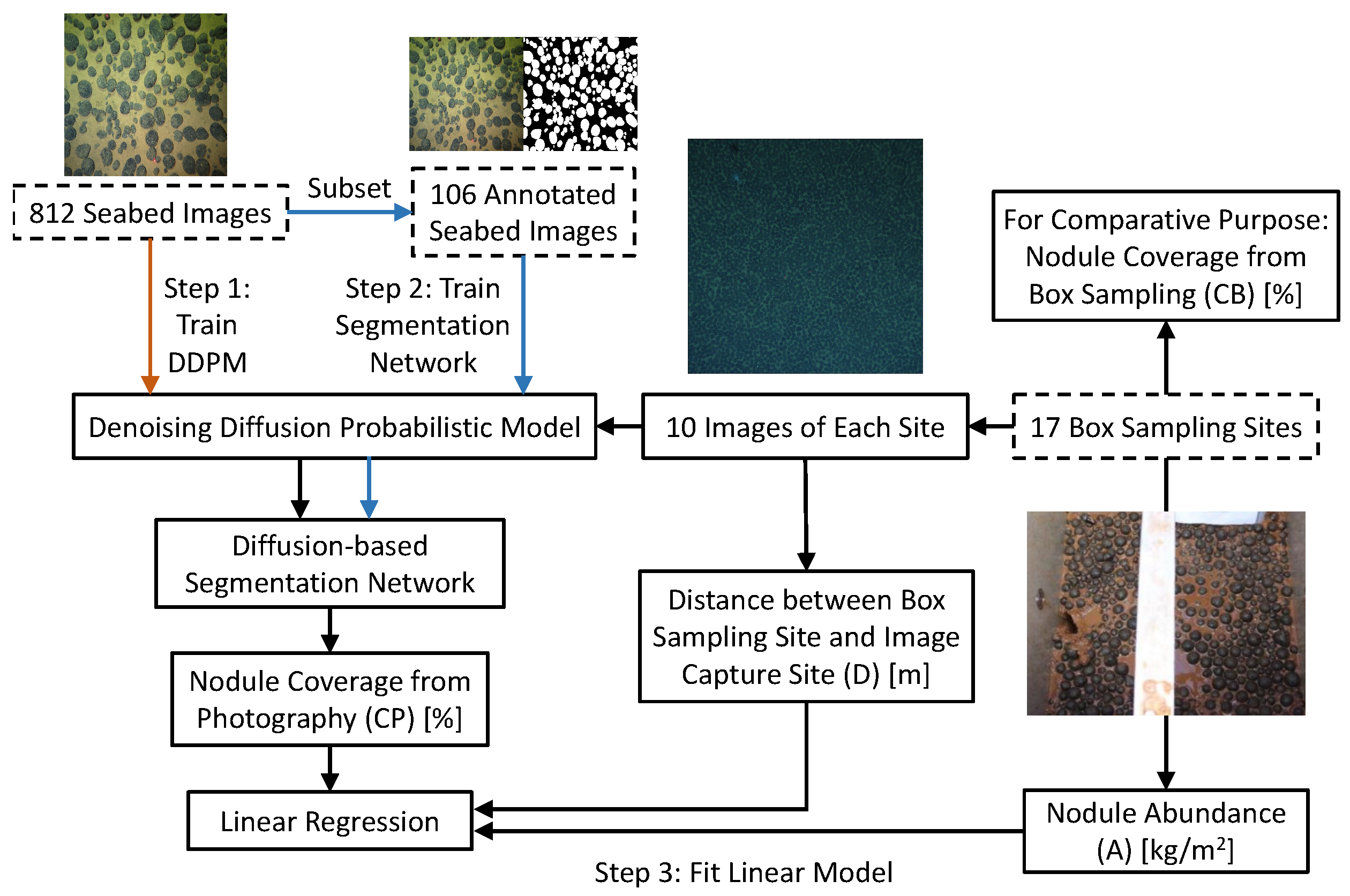
• It is the first utilization of a DDPM for extracting features in seabed nodule images, exhibiting its effectiveness in capturing high-level semantic information for accurate segmentation;
• After training on a large set of unlabeled seabed nodule images, the DDPM has the capability to generate synthetic images that closely resemble real images;
• We introduce an efficient semantic segmentation network that harnesses diffusion-based features, demonstrating strong generalization capabilities.

2. Related Works

2.1. Seabed Nodule Image Segmentation

In the 1960s, the estimation of polymetallic nodules through underwater photography marked the beginning of research in this field. Early methods primarily relied on specialized knowledge and involved studying the morphology and distribution of nodules in underwater images through geochemical studies and descriptive analysis [15]. To achieve accurate estimations of the number of nodules and quantitatively assess mineral coverage, various methods were developed, including point counting, electronic planimeters, and image processing techniques [6]. These approaches aimed to enhance the efficiency and accuracy of seabed mineral assessment.

Traditional image segmentation methods for seabed mineral analysis rely on handcrafted lower-level feature extractors such as thresholding, clustering, and region growing. Due to the absence of distinct bimodal distributions in the histograms of seabed images, employing a simple global thresholding technique leads to unsatisfactory results. Park et al. [16] employed distinctive thresholds to segment various images, leveraging the observation that image variances differ across pictures with varying nodule densities. They further predicted nodule abundance using a simple proportional function based on the coverage calculated through segmentation. Histogram equalization is known to enhance the overall brightness of an image, but it results in the loss of some detailed information. To overcome the challenge of coverage accuracy in the seabed black connected domain, Ma et al. [17] proposed a solution by adjusting the brightness equalization algorithm, defining a region of interest, and utilizing the window histogram equalization algorithm. Prabhakaran et al. [18] enhanced low-light underwater images using histogram equalization and contrast-limited adaptive histogram equalization, followed by multiscale template matching for nodule detection. Mao et al. [19] first enhanced the contrast between the foreground and background through grayscale stretching and Gaussian filtering. They then subtracted the background gray value from the grayscale image and restored the nodules’ boundaries using morphological operations. This method effectively eliminates uneven illumination and repairs the morphology of nodules, demonstrating its applicability and stability. Vijayalakshmi et al. [20] proposed a method that utilizes gradient-based joint histogram equalization. The approach involves extracting edge information using a multiscale-based dark pass filter and computing a joint histogram using both the edge information and the low-contrast image. The resulting discrete function is then mapped to a uniform distribution to obtain the final enhanced image. The experimental results demonstrate enhanced contrast and preservation of edge details using this approach. They further proposed a two-dimensional histogram equalization technique based on edge detail to both enhance contrast and maintain the image’s natural appearance [21]. The method utilizes the total variational (TV)/L1 decomposition method to extract detailed information from the low-contrast image. A two-dimensional histogram is constructed using the detailed image, and the cumulative distribution function (CDF) is determined. The CDF is then transferred to distribute the intensities across the entire dynamic range, resulting in an improved image. Wasilewska-Błaszczyk et al. [14] utilized coverage, along with other factors, to predict abundance using general linear models. Schoening et al. [22] introduced a compact-morphology-based polymetallic nodule delineation method that calculates the compactness curve and its first derivative of the seabed mineral image for nodule segmentation. Additionally, ellipsoids are fitted to each nodule, enabling the assessment of grain size. Ye et al. [23] proposed a nonlinear region K-means segmentation method to mitigate the effect of water dispersion. This approach employs spatial grayscale histogram-based Mahalanobis distance as metrics for clustering and updates cluster centers using the winner-take-all strategy. To address the issue of sensitivity to speckle noises, Wang et al. [24] proposed a segmentation scheme that combines the Markov random field model with Hard C-means clustering and further optimized the parameters using simulated annealing. Schoening et al. [25] employed histogram equalization to enhance the color contrast in all transect images, followed by the creation of a feature representation for each pixel, taking its neighborhood into account. Finally, they utilized a hyperbolic self-organizing maps (HSOM) approach to estimate mineral coverage. While HSOM performs well in detecting large nodules, it may fall short in adequately segmenting smaller-sized nodules. Kuhn et al. [26] utilized the Euclidean distance to calculate the distance map and determine the center of individual nodules. They employed a heuristic approach and deformable models to fit the contour of the nodules. This method demonstrates effectiveness in accurately segmenting small nodules. Schoening et al. [27] introduced a heuristic evolutionary tuned segmentation using cluster co-occurrence and a convexity criterion (ES4C) algorithm. This method leverages learning vector quantization to group visual features into clusters. Subsequently, an evolutionary algorithm assigns cluster prototypes to classes based on morphological compactness and feature similarity.

Deep learning algorithms, renowned for their ability to extract underlying relationships from data, have shown significant advancements in feature extraction compared to traditional methods. In the context of seabed mineral image segmentation, machine learning techniques have gained prominence. Among these techniques, convolutional neural networks (CNNs) stand out as powerful algorithms for comprehending image content. CNNs have exhibited remarkable potential in various image-related tasks, including pattern recognition, image interpretation, and image classification. As such, the application of CNNs in the field of seabed polymetallic nodule resource assessment aligns with the objective of leveraging advanced deep learning methods. Ciresan et al. [28] made the first attempt to apply CNNs for semantic segmentation, using image patches centered on each pixel to predict their classes. However, the CNNs used lacked depth, limiting their ability to capture abstract features relevant to image semantics. To address this, Long et al. [29] introduced fully convolutional neural networks (FCNs), which eliminated fully connected layers and revolutionized speed and applicability. FCNs also employ skip architectures that enable information to flow, which would otherwise be lost due to max-pooling layers or dropout, allowing shallow information to be retained at deeper levels. Despite their advantages, FCNs struggle with global context knowledge and multiscale processing. To overcome these limitations, Ronneberger et al. [30] proposed an encoder–decoder architecture known as U-Net. The encoder gradually reduces spatial dimensions with pooling layers, while the decoder recovers object details and spatial dimensions. Additionally, skip connections directly connect the decoder with the same level of encoder, enhancing information flow. U-Net has exhibited promising results in various applications and addresses the challenges in semantic segmentation. Song et al. [7] made contributions by enhancing the decoder of the U-Net architecture. They introduced upsampling and feature map fusion techniques, resulting in smoother nodule boundaries. However, one limitation of semantic segmentation models is their inability to directly estimate nodule abundance or size, as they primarily focus on obtaining nodule coverage. Unlike the existing segmentation paradigms, Girshick et al. [31] proposed the region-based convolutional neural network (R-CNN) as a breakthrough in object detection. This paradigm enables separate detection of all objects within the image and can be extended to instance segmentation. Expanding upon R-CNN, He et al. [32] introduced Mask R-CNN, a two-stage instance segmentation model that identifies and separates individual objects within an image. Dong et al. [8] applied Mask R-CNN to perform seabed nodule image segmentation. By leveraging an instance segmentation model, each nodule in the image could be individually separated, enabling straightforward calculation of abundance and nodule size based on the altitude information of the underwater camera. However, due to its two-stage structure, the model’s processing speed is contingent on the number of nodules present in the input image, posing challenges when dealing with dense nodule images.

2.2. Diffusion Models

Diffusion models are a class of generative models that approximate the distribution of real images using a Markov process [33] (see Figure 2). The image generation process consists of a forward diffusion process and a backward denoising process. During the forward process, each input image undergoes progressive degradation through the addition of noise until it eventually becomes pure Gaussian noise. Conversely, the backward process aims to restore the original image by iteratively removing the noise. At each time step, a neural network learns to subtract the noise. Notably, Ho et al. [34] proposed a novel approach of estimating the noise in the image during the backward process instead of the mean. Additionally, Nichol et al. [35] introduced the concept of learning variances in the backward process and presented an improved noise schedule. These advancements have propelled diffusion models to surpass generative adversarial networks (GANs) in terms of generative quality and diversity. Baranchuk et al. [10] demonstrated that DDPMs can also serve as effective representation learners, achieving state-of-the-art performance in few-shot semantic segmentation tasks. In this paper, we explore the applicability of diffusion models in seabed mineral segmentation. In the subsequent sections, we provide a brief overview of diffusion models.

3. Model

We present a novel two-stage model for seabed semantic segmentation, as illustrated in Figure 3. In the first stage, we employ DDPM as the backbone to extract informative image features. The second stage consists of our custom-designed segmentation network.

3.1. Denoising Diffusion Probabilistic Model

DDPM contains a forward diffusion process $q(x_t\mid x_{t-1})$, gradually corrupting data from given distribution $x_0\sim q\left(x_0\right)$ into a normal distribution and a learned reverse denoising process $p_{\theta }(x_{t-1}\mid x_t)$ that transforms the normal distribution back into the given data.

Forward process q is used to obtain the noise versions $x_1,x_2,\dots ,x_T$ from different time step t by the following nonhomogeneous Markov process:

$$q(x_t\mid x_{t-1})=\mathcal{N}(x_t;\sqrt{1-{\beta }_t}{x}_{t-1},{\beta }_t\mathbf{I}),\forall t\in \{1,\dots ,T\}$$

(1)

where T is the number is diffusion steps, and ${\beta }_1,\dots ,{\beta }_T$ are hyperparameters standing for a variance schedule. Importantly, by defining ${\alpha }_t=1-{\beta }_t$ and ${\overline{\alpha }}_t={\prod }_{s=0}^t{\alpha }_s$, we can directly obtain an arbitrary step of the noise $x_t$ from the input $x_0$ using the following expression:

$$q(x_t\mid x_0)=\mathcal{N}\left(x_t;\sqrt{{\overline{\alpha }}_t}{x}_0,\left(1-{\overline{\alpha }}_t\right)\mathbf{I}\right)$$

(2)

$$x_t=\sqrt{{\overline{\alpha }}_t}{x}_0+\sqrt{1-{\overline{\alpha }}_t}ϵ,ϵ\sim \mathcal{N}(0,\mathbf{I})$$

(3)

If we begin with a Gaussian noise $x_T\sim \mathcal{N}(0,\mathbf{I})$ and proceed with the reverse steps $p(x_{t-1}\mid x_t)=\mathcal{N}\left(x_{t-1};\mu (x_t,t),\Sigma (x_t,t)\right)$, we can generate new samples from the data distribution $q\left(x_0\right)$. However, $q(x_{t-1}\mid x_t)$ depends on the entire data distribution, and we approximate these steps using the following:

$$p_{\theta }\left(x_{t-1}\mid x_t\right)=\mathcal{N}\left(x_{t-1};{\mu }_{\theta }\left(x_t,t\right),{\Sigma }_{\theta }\left(x_t,t\right)\right)$$

(4)

We utilize a neural network that takes the noisy image $x_t$ and time step embedding t as inputs and learns to predict the mean ${\mu }_{\theta }(x_t,t)$ and the covariance ${\Sigma }_{\theta }(x_t,t)$ of the distribution. In practice, the model predicts the noise component ${ϵ}_{\theta }(x_t,t)$ at the step t, and the mean of the distribution ${\mu }_{\theta }(x_t,t)$ is a linear combination of the noise component and $x_t$. Additionally, the covariance ${\Sigma }_{\theta }(x_t,t)$ can be either fixed or learned. The denoising model ${ϵ}_{\theta }(x_t,t)$ is parameterized by U-Net architecture, as proposed in [35].

The inference process is defined as the reverse of the Markovian diffusion process. It starts from Gaussian noise $x_T$ and iteratively denoises $x_t$ at each time step t to recover $x_{t-1}$. Using the Bayes theorem, we can calculate the posterior $q\left(x_{t-1}|x_t,x_0\right)$ by the following:

$$q\left(x_{t-1}|x_t,x_0\right)=\mathcal{N}\left(x_{t-1};{\tilde{\mu }}_t\left(x_t,x_0\right),{\tilde{\beta }}_t\mathbf{I}\right)$$

(5)

where ${\tilde{\beta }}_t$ is $\frac{1-{\overline{\alpha }}_{t-1}}{1-{\overline{\alpha }}_t}{\beta }_t$, and ${\tilde{\mu }}_t\left(x_t,x_0\right)$ is $\frac{\sqrt{{\overline{\alpha }}_{t-1}}{\beta }_t}{1-{\overline{\alpha }}_t}{x}_0+\frac{\sqrt{{\alpha }_t}\left(1-{\overline{\alpha }}_{t-1}\right)}{1-{\overline{\alpha }}_t}{x}_t$.

The diffusion model serves as a powerful feature extractor for seabed nodule images. Starting with an input image $x_0\in {\mathbf{R}}^{h\times w\times 3}$, we utilize the noise predictor ${ϵ}_{\theta }(x_t,t)$ to derive feature representations. Firstly, we generate $x_t$ by introducing Gaussian noise to $x_0$, following the procedure defined in Equation (2). Subsequently, we feed the resulting noise $x_t$ into the predictor ${ϵ}_{\theta }(x_t,t)$, which is parameterized by the U-Net architecture. We capture the intermediate activations of U-Net and utilize them as inputs for our segmentation network. Specifically, our feature extraction process involves capturing features at multiple scales, including $h\times w$, $h/2\times w/2$, $h/4\times w/4$, $h/8\times w/8$, and $h/16\times w/16$ dimensions. We also utilize different time steps.

3.2. Diffusion-Based Segmentation Network

In the second stage of our approach, we propose a segmentation network composed of three main blocks: time steps hybrid block (TSHB), upsampling convolutional block (UCB), and convolutional residual block (CRB). The architecture of each block is illustrated in Figure 4a–c, respectively. The time steps hybrid block consists of two sequences of 3 × 3 convolutional layers, batch normalization layers, and ReLU layers. This block is designed to merge features from different time steps within a certain DDPM decoder block. The upsampling convolutional block includes an upsampling layer, a convolutional layer, a batch normalization layer, and a ReLU layer. It is responsible for upsampling the lower-resolution features to match the resolution of higher ones. The convolutional residual block contains two paths. One path consists of two sequences of 3 × 3 convolutional layers, batch normalization layers, and ReLU layers; in contrast, the other path contains a single sequence. The outputs from these two paths are combined by element-wise addition and are further processed by a batch normalization layer.

The segmentation network utilizes the feature representations obtained from the pretrained diffusion model and aims to predict the binary mask. Initially, the features from different time steps within a certain DDPM decoder block are merged together using the TSHB, which effectively reduces the number of channels to enhance the network’s efficiency. While the deepest feature undergoes processing through a UCB to align its resolution with the higher-level feature, other features, except for the deepest one, are merged with the upsampled feature from the UCBs. This merging process facilitates the fusion of multiscale semantic information, achieved through CRBs. Subsequently, the merged features are directed along two paths: one path involves iterative upsampling by a scale factor of 2 to merge with corresponding larger features, while the other path undergoes direct upsampling to match the resolution of the input image. These two paths ensure that the network achieves a robust segmentation effect. Finally, the features upsampled from different resolutions pass through a 1 × 1 convolutional layer to predict every pixel’s category.

3.3. Linear Regression Model

The segmentation network classifies both the background and nodule classes, enabling us to calculate nodule coverage by determining the ratio of nodule pixels to the total number of pixels in the image. Given the equal importance of nodule abundance and nodule coverage, we utilize linear regression models to assess nodule abundance. Linear regression is a statistical technique used to model the relationship between dependent and independent variables [36]. The linear regression model is expressed as follows:

$$y={\beta }_0+{\beta }_1{x}_1+\dots +{\beta }_n{x}_n$$

(6)

where y represents the dependent variable, $x_1,\dots ,x_n$ represent the independent variables, and the coefficients ${\beta }_0,\dots ,{\beta }_n$ are regression coefficients. In our study, we employ linear regression models to capture the relationship between nodule abundance and coverage.

4. Experiment

4.1. Dataset

Our dataset comprises 812 images of seabed nodules captured under various conditions, including different areas, light intensities, depths, and shooting angles (as depicted in the leftmost eight images in Figure 5). The images are captured using a camera mounted on the Ocean Floor Observatory System (OFOS), which is positioned directly above the nodules. Due to the absence of sunlight in the deep ocean, halogen lamps on the OFOS are used for illumination, resulting in the presence of darkness around the images. Out of the dataset, 106 images were annotated with fine-grained semantic masks generated using Labelme. The dataset contains one category, which is the nodule. All images were resized to a dimension of 512 × 512 pixels. For training the DDPM backbone, the first stage of our segmentation model, we utilized the entire 812 images. In the seconde stage, we randomly selected 86 labeled images for the training set, whereas the remaining 20 labeled images were designated as the testing set.

The box sample dataset contains 17 sample sites, each providing data on nodule abundance and coverage.

Table 1. Statistics of nodule abundance and coverage from sampling.

Statistics	Abundance (kg/m${}^{\mathbf{2}}$)	Coverage (%)
Count	17	17
Average	32.03	72.65
Median	31.4	74.4
20% Trimmed Mean	31.92	72.85
Standard Deviation	5.97	7.96
Coefficient of Variation	18.65%	10.95%
Minimum	21.1	59
Maximum	42.8	88
Range	21.7	29
Skewness	0.04	−0.12
Kurtosis	−0.41	−0.74
p-value (Shapiro–Wilk test)	0.495	0.616
W (Shapiro–Wilk test)	0.95	0.96

presents the statistical summary of these measures. The central tendency measures, including the average, median, and 20% trimmed mean, exhibit similar values for both abundance and coverage. The coefficients of variation are 18.65% and 10.95%, respectively, indicating a moderate level of variability. The skewness and kurtosis values suggest that the data align well with a normal distribution. Additionally, the p-value obtained from the Shapiro–Wilk test exceeds the chosen alpha level of 0.05, suggesting that there is insufficient evidence to reject the null hypothesis that the data follow a normal distribution. The distribution of the data can be further observed in the normal probability plots and box and whisker plots shown in Figure 6, where no outliers are present in the box and whisker plots.

To evaluate the performance of our regression model, we utilize a set of 10 images that are geographically closest to each of the box sampling sites. Due to variations in the original ocean voyage, the box sampling sites are not precisely aligned with the photography voyage, resulting in a certain distance between the images and the sampling sites. The average distance between each sampling site and its 10 nearest images ranges from 24.1 m to 575.8 m. Notably, the nodules present in these images exhibit a higher density compared to those found in the well-labeled dataset, as depicted in the rightmost eight images shown in Figure 5. Although all the images have a high resolution of 3000 × 4000 pixels, it is necessary to resize them to 512 × 512 pixels for input. Directly resizing the original images would cause the nodules to become too small to be accurately identified. Additionally, the illumination across these images is uneven, resulting in relative darkness around the image and leading to potential missed detections. Furthermore, the presence of camera distortion contributes to blurriness around the image periphery. And it is worth noting that the distribution of nodules within a single image is relatively uniform. To address these issues, we apply a preprocessing step that involves center-cropping the images to a size of 2000 × 2000 pixels and subsequently resizing them to the desired dimensions of 512 × 512 pixels.

4.2. Metrics

To evaluate the performance of our segmentation method, we employ several metrics, including accuracy, precision, recall, and IoU (intersection over union). Accuracy measures the ratio of correctly predicted pixels to the total number of pixels. Precision quantifies the proportion of correctly predicted mineral pixels among all predicted mineral pixels, while recall measures the fraction of predicted mineral pixels among all real mineral pixels. IoU evaluates the overlap between predicted and real mineral pixels. These metrics are calculated as follows:

$$\mathrm{Accuracy}=\frac{\mathrm{TP}+\mathrm{TN}}{\mathrm{TP}+\mathrm{TN}+\mathrm{FP}+\mathrm{FN}}$$

(7)

$$\mathrm{Precision}=\frac{\mathrm{TP}}{\mathrm{TP}+\mathrm{FP}}$$

(8)

$$\mathrm{Recall}=\frac{\mathrm{TP}}{\mathrm{TP}+\mathrm{FN}}$$

(9)

$$\mathrm{IoU}=\frac{\mathrm{TP}}{\mathrm{TP}+\mathrm{FP}+\mathrm{FN}}$$

(10)

where TP represents the number of correctly predicted true pixels, TN represents the number of correctly predicted false pixels, FP represents the number of wrongly predicted true pixels, and FN represents the number of wrongly predicted false pixels.

The coefficient of determination (R${}^2$), mean absolute error (MAE), mean absolute percentage error (MAPE), and root mean squared error (RMSE) are used to evaluate the linear regression model. R${}^2$ represents the proportion of the variation in the dependent variable that can be explained by the independent variables. MAE measures the average size of errors. MAPE measures the size of errors in percentage terms. RMSE represents the standard deviation of prediction errors. These metrics are calculated as follows:

$${\mathrm{R}}^2=1-\frac{{\sum }_i{(y_i-{\widehat{y}}_i)}^2}{{\sum }_i{(y_i-\overline{y})}^2}$$

(11)

$$\mathrm{MAE}=\frac{1}{n}\sum _i\left|y_i-{\widehat{y}}_i\right|$$

(12)

$$\mathrm{MAPE}=\frac{1}{n}\sum _i\frac{\left|y_i-{\widehat{y}}_i\right|}{y_i}$$

(13)

$$\mathrm{RMSE}=\sqrt{\frac{1}{n}\sum _i{(y_i-{\widehat{y}}_i)}^2}$$

(14)

where n is the count of data points, ${\widehat{y}}_i$ is the predicted value, $y_i$ is the observed value, and $\overline{y}$ is the mean of all the observed value.

4.3. Implementation Details

In our DDPM backbone, we adopt the same architecture as Nichol et al. [35] for approximating ${ϵ}_{\theta }$. The hyperparameters of the model architecture are as follows: 1000 diffusion steps, a linear noise schedule, 256 base model channels, 2 residual blocks, attention resolutions of 32, 16, and 8, a dropout rate of 0.1, 64 attention head channels, and a learning rate of 1 × 10${}^{-5}$. Additionally, we utilize residual blocks for both upsampling and downsampling, and apply scale shift normalization.

For the second stage of the semantic segmentation network, we utilize representations from the middle blocks 7, 10, 13, 16, 17 of the U-Net decoder, as well as the later time steps 50, 100, 150 from the reverse diffusion process. The batch size is set to 2, and the model is trained for 100 epochs using RMSProp as the optimizer. We initialize the learning rate to 1 × 10${}^{-6}$, set the weight decay to 1 × 10${}^{-8}$, and the learning momentum to 0.999.

4.4. Results and Discussion

In the first stage, we train DDPM using our seabed nodule image dataset, consisting of mostly unlabeled images and a few labeled images. As shown in Figure 7, the generated images closely resemble real seabed mineral images, accurately depicting sediment, nodules, and even red laser points that are commonly observed in real-world scenarios. Real underwater images often exhibit dark yellow, dark blue, and dark green tones, accompanied by black shadows at the image edges due to underwater lighting conditions. The synthesized images effectively restore the seabed illumination, maintaining the overall color tone of the actual images. While the hue of some synthesized images aligns with that of real images, variations in color saturation and brightness have not been observed in our dataset. Nonetheless, given that underwater images are artificially illuminated, these synthesized images still hold reliability and may also appear in other datasets or future underwater survey images. These distinctive lighting conditions offer promising opportunities for the development of seabed image enhancement models in the future study. The synthesized images also demonstrate the DDPM’s ability to generate nodules with varying distribution densities, accurately reflecting the density in both dense and sparse situations. Moreover, the model effectively restores the burial of minerals in real seabed images. Notably, in synthetic images with larger and sparsely distributed nodules (which can be considered as the camera being closer to the seabed), the shadows of the nodules can even reflect that they have heights.

These generated images exhibit a diverse range of distributions and illuminations, further validating the realism of the synthetic data. Although the original purpose of the model is to generate images, we repurpose it as a feature extractor in our approach. The high quality of these synthetic images is a testament to our model’s ability to effectively learn the intricate features of seabed nodule images. Figure 8 showcases the multiscale features obtained from different time steps and decoder blocks, highlighting the proficiency of the diffusion model in extracting features. Notably, the smaller-scale representations capture abstract features, whereas the larger ones discern detailed patterns such as edges. The deepest features are extracted from the deepest layer of the DDPM’s U-Net structure (as depicted in the last row of Figure 8). These features have the highest number of channels but the smallest size, equivalent to 1/16 of the input image dimensions (16 × 16 in our model). They capture more abstract and large-scale image features. While each pixel in these deep features represents information from a larger receptive field, fine details like edges are absent due to their small scale. Deep semantic information, although challenging to interpret directly, is crucial in the model. Moving from deep to shallow layers, the number of channels gradually decreases, and the image size increases to match the input dimensions. The shallowest features, obtained from the shallowest layer (as depicted in the first row of Figure 8), contain the most specific and detailed information. Being closer to the output layer, these shallow features are more easily understood by humans. They possess a smaller receptive field, limiting their ability to capture the overall image structure, but excel at capturing fine details such as color, texture, edges, and corners. The sharp definition of mineral edges in this layer exemplifies the model’s precise segmentation capabilities.

In the evaluation of our two-stage segmentation model, we compare its performance to several prior approaches commonly used for segmenting seabed mineral images.

Table 2. Comparison of segmentation performance between our proposed model and others.

Method	Accuracy	Precision	Recall	IoU
U-Net [8]	96.97	84.17	79.02	71.12
Improved U-Net [8]	96.80	82.94	79.97	71.38
CGAN [8]	95.91	79.28	80.10	67.51
Mask R-CNN [8]	97.24	83.51	85.58	74.73
Ours	96.94	87.30	86.49	76.67

presents a comparison of the validation results obtained by different models. The diffusion-based segmentation network achieves an accuracy, precision, recall, and IoU of 96.94, 87.30, 86.49, and 76.67, respectively, on the test set. Overall, our proposed method outperforms the other approaches. The diffusion-based segmentation network demonstrates slightly lower accuracy compared to U-Net and Mask R-CNN, with a maximum difference of 0.3. However, it outperforms Improved U-Net and CGAN. In terms of precision, the diffusion-based segmentation network surpasses all other models and achieves a value of 84.17, exceeding the second-ranked U-Net model by 3.1. For recall, the diffusion-based segmentation network slightly outperforms the Mask R-CNN model by 0.91 and significantly outperforms other models by at least 6. In terms of IoU, the diffusion-based segmentation network outperforms all other models, surpassing the second-ranked Mask R-CNN model by 1.94. Although the diffusion-based segmentation network falls slightly short of the current optimal accuracy level, it is only marginally weaker than the best-performing model. However, when considering other metrics, the diffusion-based segmentation network consistently outperforms the current state-of-the-art models. Therefore, overall, we are highly satisfied with the performance of our model.

Given that the mineral dataset comprises a significant number of small nodules, we utilize the shallow blocks of the U-Net decoder. These blocks feature relatively larger feature maps, enabling better recognition of the small objects, as shown in Figure 8. However, it is important to note that the shallower blocks also contain more Gaussian noise compared to the deeper ones, which can lead to misjudgments. Taking into consideration the aforementioned points, our diffusion-based method surpasses the other approaches and proves to be effective in the task of mineral image segmentation.

To utilize the linear regression model for predicting nodule abundance, we first use each segmentation model to predict the nodule coverage of images that are geologically close to each box sampling point. As these images are unlabeled, the segmentation performance can only be assessed visually and cannot be quantitatively evaluated using metrics. Additionally, these images are excluded from model training, allowing the model’s performance on these images to demonstrate its generalization ability. Figure 9 illustrates the performance of U-Net, Improved U-Net, CGAN, and the diffusion-based segmentation network in different image scenarios. Overall, the diffusion-based segmentation network outperforms the other models. U-Net and Improved U-Net show similar results, while the CGAN model’s segmentation performance is unsatisfactory. In images with a less dense distribution and the nodules exhibiting a spheroidal shape (as shown in the first and second rows of Figure 9), our model, along with Improved U-Net and U-Net, achieves good performance in these cases. The diffusion-based segmentation network successfully identifies buried nodules in overexposed images, such as the ones located at the bottom center of the second row of Figure 9, while other models fail to recognize them. In densely distributed nodule images (as shown in the third row of Figure 9), each nodule occupies only a few pixels due to resolution limitations, making it challenging to accurately identify individual nodules. As a result, the boundaries between two nodules in the segmentation results are not as clear. Both the U-Net and Improved U-Net tend to merge multiple independent nodules within a small region into a single large nodule, which is incorrect segmentation. However, visually, this is not the case. Our proposed DDPM model does not exhibit this phenomenon, and effectively distinguishes between different nodules, although in some regions with strong adhesion between the boundaries of multiple nodules. In the fourth row of Figure 9, all models struggle to accurately segment nodules in the bottom region. The diffusion-based segmentation network slightly outperforms the others in this aspect, and there are no instances of misidentification as a single large nodule, as previously mentioned. For images with lower brightness, such as those in the fifth and sixth rows of Figure 9, our segmentation results are generally superior. The U-Net and Improved U-Net models fail to recognize the nodule features in the dark regions and mistakenly identify the surroundings as nodules. These models also exhibit the tendency to misidentify dense nodules as a single large nodule. In contrast, the diffusion-based segmentation network performs well in these dark images, with segmentation results that are almost indistinguishable from those obtained under normal brightness conditions. This indicates that the diffusion-based segmentation network effectively overcomes the brightness issue. Our first-stage generative model has the capability of generating images with different lighting conditions and nodule distributions, even generating plausible images that are not present in the dataset. The segmentation results demonstrate that the second-stage segmentation model successfully captures the features of nodule images under different conditions and accurately segments nodule images in various conditions. During actual underwater survey, the distribution of nodules and lighting conditions are challenging to predict, often requiring significant efforts for camera configuration. By utilizing our model, these issues can be addressed at the post-processing stage, leading to cost savings.

We utilize the nodule coverage calculated by our diffusion-based segmentation model to predict nodule abundance. The variables used in the linear models are shown schematically in Figure 1. Considering that there are 10 images for each sampling site, we calculate the mean coverage of the 10 images as the independent variable. The box sampling abundance is considered the dependent variable. Hence, we employ the following linear model:

$$\mathrm{A}={\beta }_0+{\beta }_1\mathrm{CP}$$

(15)

where A represents the abundance obtained from box sampling, and CP represents the predicted coverage from seabed photography.

Due to the difference in distance between the sampling site and the image capture site, we incorporate distance as an additional independent variable. Hence, the linear regression model takes the following form:

$$\mathrm{A}={\beta }_0+{\beta }_1\mathrm{CP}+{\beta }_2\mathrm{D}$$

(16)

where D represents the mean distance of the 10 images.

Logarithmic transformation in regression models is commonly used to address issues related to nonlinear relationships between independent and dependent variables, which can improve model performance. Therefore, we apply a natural logarithmic transformation to the independent variable CP. The modified regression models are as follows:

$$\mathrm{A}={\beta }_0+{\beta }_{1}ln\left(\mathrm{CP}\right)$$

(17)

$$\mathrm{A}={\beta }_0+{\beta }_{1}ln\left(\mathrm{CP}\right)+{\beta }_2\mathrm{D}$$

(18)

For comparison purposes, we also utilize a linear regression model to analyze the relationship between nodule abundance and coverage obtained both from box sampling. Since both variables are derived from the same box sampling site, distance is not considered as an independent variable. Additionally, we apply a logarithmic transformation to the coverage variable. The comparison models are expressed as follows:

$$\mathrm{A}={\beta }_0+{\beta }_1\mathrm{CB}$$

(19)

$$\mathrm{A}={\beta }_0+{\beta }_{1}ln\left(\mathrm{CB}\right)$$

(20)

where CB represents the coverage obtained from box sampling.

We input the data A, CB, CP, and D into the aforementioned linear models for fitting. The results of the fitting process and their corresponding metrics are presented in

Table 3. Linear regression models between nodule abundance (A) and coverage from photography (CP), coverage from box sampling (CB), distance between the sampling site, and the image capture site (D).

Coverage Type	Linear Regression Model	R${}^{\mathbf{2}}$	MAE	MAPE	RMSE
Coverage from photography	$\mathrm{A}=1.17\mathrm{CP}-40.4$	0.221	4.059	0.138	5.273
	$\mathrm{A}=72.35ln\left(\mathrm{CP}\right)-266.64$	0.220	4.062	0.138	5.277
	$\mathrm{A}=1.34\mathrm{CP}+0.0031\mathrm{D}-52.26$	0.223	3.988	0.136	5.267
	$\mathrm{A}=85.24ln\left(\mathrm{CP}\right)+0.0036\mathrm{D}-320.82$	0.222	3.981	0.135	5.269
Coverage from box sampling	$\mathrm{A}=0.49\mathrm{CB}-3.67$	0.428	3.358	0.114	4.519
	$\mathrm{A}=34.86ln\left(\mathrm{CB}\right)-117.16$	0.423	3.425	0.116	4.539

. Based on the regression results, it can be observed that while the prediction accuracy of nodule abundance using coverage from seabed photography is not as high as that from box sampling, it still demonstrates a certain level of predictive capability. Incorporating the distance between the sampling site and the image capture site slightly improves the model’s performance. On the other hand, the logarithmic transformation does not consistently enhance the model’s performance; in some cases, it even diminishes it. This can be attributed to the significant variation in seabed nodule distributions resulting from the considerable distance between the sampling site and image capture site, which limits the predictive accuracy of abundance. It is worth noting that coverage alone is not the sole factor associated with nodule abundance. To establish a more robust and reliable relationship, other factors, such as the extent to which nodule is buried by sediment, should be taken into consideration.

5. Conclusions

In this study, we propose a novel semantic segmentation method for seabed nodule assessment based on diffusion models. Traditional image segmentation methods face challenges in applying them to seabed images due to issues like color distortion, uneven illumination, diverse nodule distribution, and sedimentary burial. Diffusion models have shown promising results in feature extraction and few-shot semantic segmentation tasks, making them suitable for seabed image segmentation. Therefore, we utilized a diffusion model in conjunction with our proposed segmentation network on a seabed nodule dataset. The segmentation results demonstrate that our proposed model effectively segments nodules despite extreme illumination conditions and high density. Notably, our method performs well even with limited annotated images, and it can adapt to seabed nodule images captured from different areas, enabling the evaluation of polymetallic nodule coverage. Additionally, we employ a linear model to predict nodule abundance based on the coverage derived from seabed nodule image segmentation. This indicates that our model can estimate nodule coverage and abundance in seabed photographs taken outside of sampling sites. However, it should be noted that our method faces limitations in processing high-resolution seabed images due to the resolution constraints of the DDPM backbone. Moreover, challenges such as nodule adhesion and interference from marine organisms require further research and investigation.

References

1. Hein, J.R.; Mizell, K.; Koschinsky, A.; Conrad, T.A. Deep-ocean mineral deposits as a source of critical metals for high- and green-technology applications: Comparison with land-based resources. Ore Geol. Rev. 2013, 51, 1–14. [Google Scholar] [CrossRef]
2. Ma, W.; Zhang, K.; Du, Y.; Liu, X.; Shen, Y. Status of Sustainability Development of Deep-Sea Mining Activities. J. Mar. Sci. Eng. 2022, 10, 1508. [Google Scholar] [CrossRef]
3. Kuhn, T.; Wegorzewski, A.; Rühlemann, C.; Vink, A. Composition, Formation, and Occurrence of Polymetallic Nodules. In Deep-Sea Mining: Resource Potential, Technical and Environmental Considerations; Sharma, R., Ed.; Springer International Publishing: Cham, Switzerland, 2017; pp. 23–63. [Google Scholar]
4. Hein, J.R.; Koschinsky, A.; Bau, M.; Manheim, F.T.; Kang, J.K.; Roberts, L. Cobalt-rich ferromanganese crusts in the Pacific. In Handbook of Marine Mineral Deposits; Cronan, D.S., Ed.; CRC Press: London, UK, 1999; pp. 239–280. [Google Scholar]
5. Hein, J.R.; Koschinsky, A.; Kuhn, T. Deep-ocean polymetallic nodules as a resource for critical materials. Nat. Rev. Earth Environ. 2020, 1, 158–169. [Google Scholar] [CrossRef] [Green Version]
6. Sharma, R.; Sankar, S.J.; Samanta, S.; Sardar, A.A.; Gracious, D. Image analysis of seafloor photographs for estimation of deep-sea minerals. Geo-Mar. Lett. 2010, 30, 617–626. [Google Scholar] [CrossRef]
7. Song, W.; Zheng, N.; Liu, X.; Qiu, L.; Zheng, R. An Improved U-Net Convolutional Networks for Seabed Mineral Image Segmentation. IEEE Access 2019, 7, 82744–82752. [Google Scholar] [CrossRef]
8. Dong, L.; Wang, H.; Song, W.; Xia, J.; Liu, T. Deep sea nodule mineral image segmentation algorithm based on Mask R-CNN. In Proceedings of the ACM Turing Award Celebration Conference—China ( ACM TURC 2021), Hefei, China, 30 July–1 August 2021; pp. 278–284. [Google Scholar] [CrossRef]
9. Croitoru, F.A.; Hondru, V.; Ionescu, R.T.; Shah, M. Diffusion models in vision: A survey. IEEE Trans. Pattern Anal. Mach. Intell. 2023, 1–20. [Google Scholar] [CrossRef]
10. Baranchuk, D.; Rubachev, I.; Voynov, A.; Khrulkov, V.; Babenko, A. Label-Efficient Semantic Segmentation with Diffusion Models. arXiv 2022, arXiv:2112.03126. [Google Scholar] [CrossRef]
11. Kuhn, T.; Rühlemann, C. Exploration of Polymetallic Nodules and Resource Assessment: A Case Study from the German Contract Area in the Clarion-Clipperton Zone of the Tropical Northeast Pacific. Minerals 2021, 11, 618. [Google Scholar] [CrossRef]
12. Mucha, J.; Wasilewska-Błaszczyk, M. Estimation Accuracy and Classification of Polymetallic Nodule Resources Based on Classical Sampling Supported by Seafloor Photography (Pacific Ocean, Clarion-Clipperton Fracture Zone, IOM Area). Minerals 2020, 10, 263. [Google Scholar] [CrossRef] [Green Version]
13. Wasilewska-Błaszczyk, M.; Mucha, J. Possibilities and Limitations of the Use of Seafloor Photographs for Estimating Polymetallic Nodule Resources—Case Study from IOM Area, Pacific Ocean. Minerals 2020, 10, 1123. [Google Scholar] [CrossRef]
14. Wasilewska-Błaszczyk, M.; Mucha, J. Application of General Linear Models (GLM) to Assess Nodule Abundance Based on a Photographic Survey (Case Study from IOM Area, Pacific Ocean). Minerals 2021, 11, 427. [Google Scholar] [CrossRef]
15. Glasby, G. Distribution of manganese nodules and lebensspuren in underwater photographs from the Carlsberg Ridge, Indian Ocean. N. Z. J. Geol. Geophys. 1973, 16, 1–17. [Google Scholar] [CrossRef]
16. Park, C.Y.; Park, S.H.; Kim, C.W.; Kang, J.K.; Kim, K.H. An Image Analysis Technique for Exploration of Manganese Nodules. Mar. Georesour. Geotechnol. 1999, 17, 371–386. [Google Scholar] [CrossRef]
17. Ma, X.; He, Z.; Huang, J.; Dong, Y.; You, C. An Automatic Analysis Method for Seabed Mineral Resources Based on Image Brightness Equalization. In Proceedings of the 2019 3rd International Conference on Digital Signal Processing, Jeju Island, Republic of Korea, 24 February 2019; pp. 32–37. [Google Scholar] [CrossRef]
18. Prabhakaran, K.; Ramesh, R.; Nidhi, V.; Rajesh, S.; Gopakumar, K.; Ramadass, G.A.; Atman, M.A. Underwater Image Processing to Detect Polymetallic Nodule Using Template Matching. In Proceedings of the Global Oceans 2020: Singapore–U.S. Gulf Coast, Biloxi, MS, USA, 5–30 October 2020; pp. 1–6. [Google Scholar] [CrossRef]
19. Mao, H.; Liu, Y.; Yan, H.; Qian, C.; Xue, J. Image Processing of Manganese Nodules Based on Background Gray Value Calculation. Comput. Mater. Contin. 2020, 65, 511–527. [Google Scholar] [CrossRef]
20. Vijayalakshmi, D.; Nath, M.K. A Novel Contrast Enhancement Technique using Gradient-Based Joint Histogram Equalization. Circuits Syst. Signal Process. 2021, 40, 3929–3967. [Google Scholar] [CrossRef]
21. Vijayalakshmi, D.; Nath, M.K. A strategic approach towards contrast enhancement by two-dimensional histogram equalization based on total variational decomposition. Multimed. Tools Appl. 2023, 82, 19247–19274. [Google Scholar] [CrossRef]
22. Schoening, T.; Jones, D.O.B.; Greinert, J. Compact-Morphology-based poly-metallic Nodule Delineation. Sci. Rep. 2017, 7, 13338. [Google Scholar] [CrossRef] [PubMed] [Green Version]
23. Ye, Z. Objective assessment of nonlinear segmentation approaches to gray level underwater images. Int. J. Graph. Vis. Image Process. (GVIP) 2009, 9, 39–46. [Google Scholar]
24. Wang, Y.; Fu, L.; Liu, K.; Nian, R.; Yan, T.; Lendasse, A. Stable underwater image segmentation in high quality via MRF model. In Proceedings of the OCEANS 2015-MTS/IEEE Washington, Washington, DC, USA, 19–22 October 2015; pp. 1–4. [Google Scholar] [CrossRef]
25. Schoening, T.; Kuhn, T.; Nattkemper, T.W. Estimation of poly-metallic nodule coverage in benthic images. In Proceedings of the 41st Conference of the Underwater Mining Institute, Shanghai, China, 15–20 October 2012. [Google Scholar]
26. Kuhn, T.; Rathke, M. Report on Visual Data Acquisition in the Field and Interpretation for SMnN; Blue Mining Project; Blue Mining Deliverable D1.31; European Commission Seventh Framework Programme; Blue Mining; European Commission: Brussels, Belgium, 2017; p. 34. [Google Scholar]
27. Schoening, T.; Kuhn, T.; Jones, D.O.B.; Simon-Lledo, E.; Nattkemper, T.W. Fully automated image segmentation for benthic resource assessment of poly-metallic nodules. Methods Oceanogr. 2016, 15–16, 78–89. [Google Scholar] [CrossRef]
28. Cireşan, D.C.; Giusti, A.; Gambardella, L.M.; Schmidhuber, J. Deep neural networks segment neuronal membranes in electron microscopy images. In Proceedings of the 25th International Conference on Neural Information Processing Systems, Lake Tahoe, NV, USA, 3–8 December 2012; Volume 2, pp. 2843–2851. [Google Scholar]
29. Long, J.; Shelhamer, E.; Darrell, T. Fully convolutional networks for semantic segmentation. In Proceedings of the 2015 IEEE Conference on Computer Vision and Pattern Recognition (CVPR), Boston, MA, USA, 7–12 June 2015; pp. 3431–3440. [Google Scholar] [CrossRef] [Green Version]
30. Ronneberger, O.; Fischer, P.; Brox, T. U-Net: Convolutional Networks for Biomedical Image Segmentation. In Proceedings of the Medical Image Computing and Computer-Assisted Intervention—MICCAI 2015, Munich, Germany, 5–9 October 2015; pp. 234–241. [Google Scholar] [CrossRef] [Green Version]
31. Girshick, R.; Donahue, J.; Darrell, T.; Malik, J. Region-based convolutional networks for accurate object detection and segmentation. IEEE Trans. Pattern Anal. Mach. Intell. 2015, 38, 142–158. [Google Scholar] [CrossRef] [PubMed]
32. He, K.; Gkioxari, G.; Dollár, P.; Girshick, R. Mask r-cnn. In Proceedings of the 2017 IEEE International Conference on Computer Vision (ICCV), Venice, Italy, 22–29 October 2017; pp. 2961–2969. [Google Scholar]
33. Sohl-Dickstein, J.; Weiss, E.A.; Maheswaranathan, N.; Ganguli, S. Deep Unsupervised Learning using Nonequilibrium Thermodynamics. In Proceedings of the 32nd International Conference on Machine Learning, Lille, France, 7–9 July 2015; Volume 37, pp. 2256–2265. [Google Scholar]
34. Ho, J.; Jain, A.; Abbeel, P. Denoising diffusion probabilistic models. In Proceedings of the 34th International Conference on Neural Information Processing Systems, Red Hook, NY, USA, 6 December 2020; pp. 6840–6851. [Google Scholar]
35. Nichol, A.Q.; Dhariwal, P. Improved Denoising Diffusion Probabilistic Models. In Proceedings of the 38th International Conference on Machine Learning, Virtual, 18 July 2021; Volume 139, pp. 8162–8171. [Google Scholar]
36. Freedman, D.A. Statistical Models: Theory and Practice, 2nd ed.; Cambridge University Press: Cambridge, UK, 2009. [Google Scholar]
Figure 1. Diagram of the types of data obtained from photography and box sampling used in our method.
Jmse 11 01494 g001
Figure 2. The diffusion model considered as a directed graphical model.
Jmse 11 01494 g002
Figure 3. Proposed seabed mineral segmentation model architecture: (a) denoising diffusion probabilistic model; (b) diffusion-based segmentation network.
Jmse 11 01494 g003
Figure 4. The architecture of our proposed blocks: (a) time steps hybrid block (TSHB), (b) upsampling convolutional block (UCB), (c) convolutional residual block (CRB).
Jmse 11 01494 g004
Figure 5. Seabed nodule images. The left 8 images are fine-labeled. The right 8 images are near the box sampling sites.
Jmse 11 01494 g005
Figure 6. Normal probability plots (left) and box and whisker plots (right) of nodule abundance and coverage.
Jmse 11 01494 g006
Figure 7. Images generated from DDPM.
Jmse 11 01494 g007
Figure 8. Features in different time steps t from different decoder blocks.
Jmse 11 01494 g008
Figure 9. Segmentation results of seabed nodule images that near box sampling using different seabed mineral segmentation methods: (a) image, (b) ours, (c) Improved U-Net, (d) U-Net, (e) CGAN.
Jmse 11 01494 g009