Study on the Energy Loss Characteristics of Shaft Tubular Pump Device under Stall Conditions Based on the Entropy Production Method

Abstract

This study aimed to reveal the energy loss characteristics of each part of the shaft tubular pump device (STPD) under stall conditions. Numerical simulations were conducted by using the SST k-ω turbulence model with curvature correction, and the reliability of the simulation results was verified by a model test. The entropy production method was used to evaluate and visualize the energy loss. The results show that turbulent entropy production (TEP) is the main source of energy loss in each component of the STPD, and the TEP increases significantly with the deterioration of stall. The energy loss in the impeller is mainly concentrated near the shroud and hub, while in the guide vanes it is mainly concentrated near the shroud and suction surface of the blades. In addition, with the deterioration of stall, the energy loss in the inlet of the impeller and guide vanes increases significantly. Influenced by the backflow from the impeller, there is a significant amount of energy loss at the outlet segment of the inlet passage, and the location of the high-energy-loss region is consistent with the backflow region. Affected by the flow separation vortex at the tail of the guide vanes, the energy loss in the outlet passage is mainly concentrated at the inlet segment.

1. Introduction

An axial flow pump is a typical vane pump that is widely used in the coastal plain area [1,2]. In China, the shaft tubular pump device (STPD) has been used in more than one hundred pump stations to date [3,4]. Recently, the range of water level fluctuations in coastal areas has increased due to global climate change. As a result, the STPD is required to operate at low flow conditions to provide higher head, which leads to stall phenomena.

The concept of the stall was first introduced in the study of airfoil lift. In 1955, Emmons [5] found the same phenomenon in a centrifugal compressor and provided an explanation of the mechanism of stall generation. Previously, some researchers have investigated the performance curve [6,7,8], internal flow characteristics [9,10,11], and vibration [12,13] of vane pumps under stall conditions. Goltz et al. [14] conducted a test of an axial flow pump under full working conditions. They discovered that the head will suddenly decrease when the stall begins. And as the stall level intensifies, a cross-passage vortex will appear in the impeller. In addition, some studies prove that the operating condition when the slope of the head curve becomes positive is the critical stall condition [15,16,17]. Toyokura et al. [18] found that under design conditions the flow in the impeller is smooth and moves forward along the airfoil. However, under stall conditions, the radial velocity of the impeller surges, and a sudden change occurs in the performance curve. Zierke et al. [19] visualized the internal flow in the impeller and observed a horseshoe vortex. Benra [20] and Farrell et al. [21] captured the internal flow structure under stall conditions by visualization techniques and analyzed the relationship between internal flow and the performance curve. Canbaz [22] and Kan et al. [23] found that the amplitude of pressure pulsation under stall conditions increases significantly.

In these previous studies, the energy loss characteristics of each component of the axial flow pump device under stall conditions have not been studied. This is because the traditional method of energy loss calculation relies on the pressure difference between two sections, but the pressure distribution on the section is not uniform under stall conditions, so the traditional method cannot be used to evaluate the energy loss under stall conditions. In recent years, there have been a number of studies on entropy production methods [24,25,26,27], and these methods have also been used by some scholars to investigate the losses [28,29]. With its continuous improvement, the entropy production method has been increasingly applied in the field of rotating machinery [30,31,32,33,34]. Some scholars compared the entropy production method with the traditional pressure drop method and showed that the energy loss results obtained by the entropy production method are reliable and accurate [35].

At present, almost no researchers have conducted an in-depth study of the energy loss in the STPD under stall conditions. In this study, an STPD was used as the research object, the energy loss characteristics of each component were quantitatively analyzed by the entropy production method, and the high-energy-loss regions were identified. This study reveals the loss characteristics of the STPD under stall conditions and can help to reduce the energy loss.

2. Numerical Simulation and Entropy Production Method

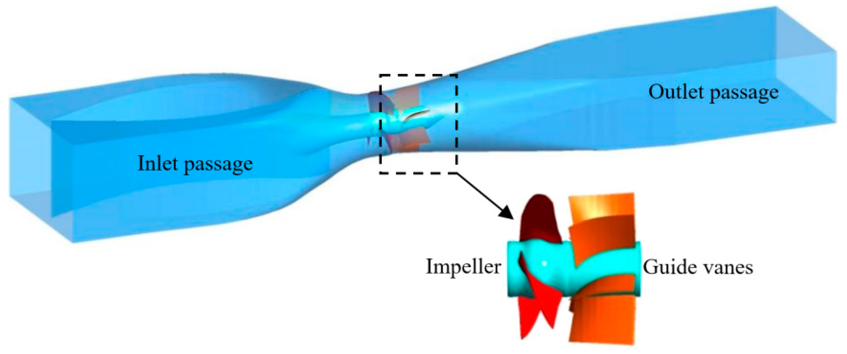
2.1. Three-Dimensional Model and Turbulence Model

The STPD consists of four parts; a three-dimensional model is shown in Figure 1. The basic parameters of the STPD are introduced in Ref. [7].

The SST k-ω turbulence model [36] was used in this study. This turbulence model has found extensive application in the field of rotating machinery [37,38].

$$\frac{\partial \left(\rho k\right)}{\partial t}+\frac{\partial \left(\rho k{u}_j\right)}{\partial x_j}=\frac{\partial }{\partial x_j}\left[\left(\mu +{\sigma }_k{\mu }_t\right)\frac{\partial k}{\partial x_j}\right]+P_k-{\beta }^{\prime }\rho k\omega ,$$

(1)

$$\frac{\partial \left(\rho \omega \right)}{\partial t}+\frac{\partial \left(\rho \omega u_j\right)}{\partial x_j}=\mathsf{\alpha }{S}^2-\beta \rho {\omega }^2+\frac{\partial }{\partial x_j}\left[\left(\mu +{\sigma }_{\omega }{\mu }_t\right)\frac{\partial \omega }{\partial x_j}\right]+2\left(1-F_1\right)\frac{\rho {\sigma }_{\omega 2}}{\omega }\frac{\partial k}{\partial x_j}\frac{\partial \omega }{\partial x_j},$$

(2)

$$F_1=\tanh \left\{{\left\{\mathrm{m}\mathrm{i}\mathrm{n}\left[\mathrm{m}\mathrm{a}\mathrm{x}\left(\frac{\sqrt{k}}{{\beta }^{\prime }\omega y},\frac{500v}{y^2\omega }\right),\frac{4{\sigma }_{\omega 2}k}{C{D}_{k\omega }{y}^2}\right]\right\}}^4\right\},$$

(3)

$$F_2=\tanh \left[{\left[\mathrm{m}\mathrm{a}\mathrm{x}\left(\frac{2\sqrt{k}}{{\beta }^{\prime }\omega y},\frac{500v}{y^2\omega }\right)\right]}^2\right],$$

(4)

$$P_k=\mathrm{m}\mathrm{i}\mathrm{n}\left({\tau }_{ij}\frac{\partial u_i}{\partial x_j},10{\beta }^{\prime }k\omega \right),$$

(5)

$${CD}_{k\omega }=\mathrm{m}\mathrm{a}\mathrm{x}\left(2\rho {\sigma }_{\omega 2}\frac{1}{\omega }\frac{\partial k}{\partial x_i}\frac{\partial \omega }{\partial x_i},{10}^{-10}\frac{500v}{y^2\omega }\right),$$

(6)

where ${\mu }_t=\frac{\rho a_{1}k}{\max \left(a_1\omega ,S{F}_2\right)}$.

Under stall conditions, the flow within the axial flow pump has high curvature and rotational intensity. Therefore, a curvature correction method provided by Spalart and Shur was used in this study [39,40,41]. The mathematical expression for the correction coefficient is as follows:

$$f_{rotation}=\left(1+c_{r1}\right)\frac{2r^{*}}{1+r^{*}}\left[1-c_{r3}{\tan }^{-1}\left(c_{r2}\tilde{r}\right)\right]-c_{r1},$$

(7)

$$r^{*}=\overline{S}/\overline{\mathsf{\Omega }},$$

(8)

$$\tilde{r}=\left[2{\mathsf{\Omega }}_{ik}{S}_{jk}{\left(D\overline{S}/Dt\right)}_{ij}\right]/\overline{\mathsf{\Omega }}{D}^3,$$

(9)

$$D^2=\mathrm{m}\mathrm{a}\mathrm{x}\left(\overline{S^2},0.09{\omega }^2\right),$$

(10)

$$\overline{S}=\sqrt{2S_{ij}{S}_{ij}},$$

(11)

$$\overline{\mathsf{\Omega }}=\sqrt{2{\mathsf{\Omega }}_{ij}{\mathsf{\Omega }}_{ij}},$$

(12)

where $c_{r1}=1$, $c_{r2}=$2, $c_{r3}=1$.

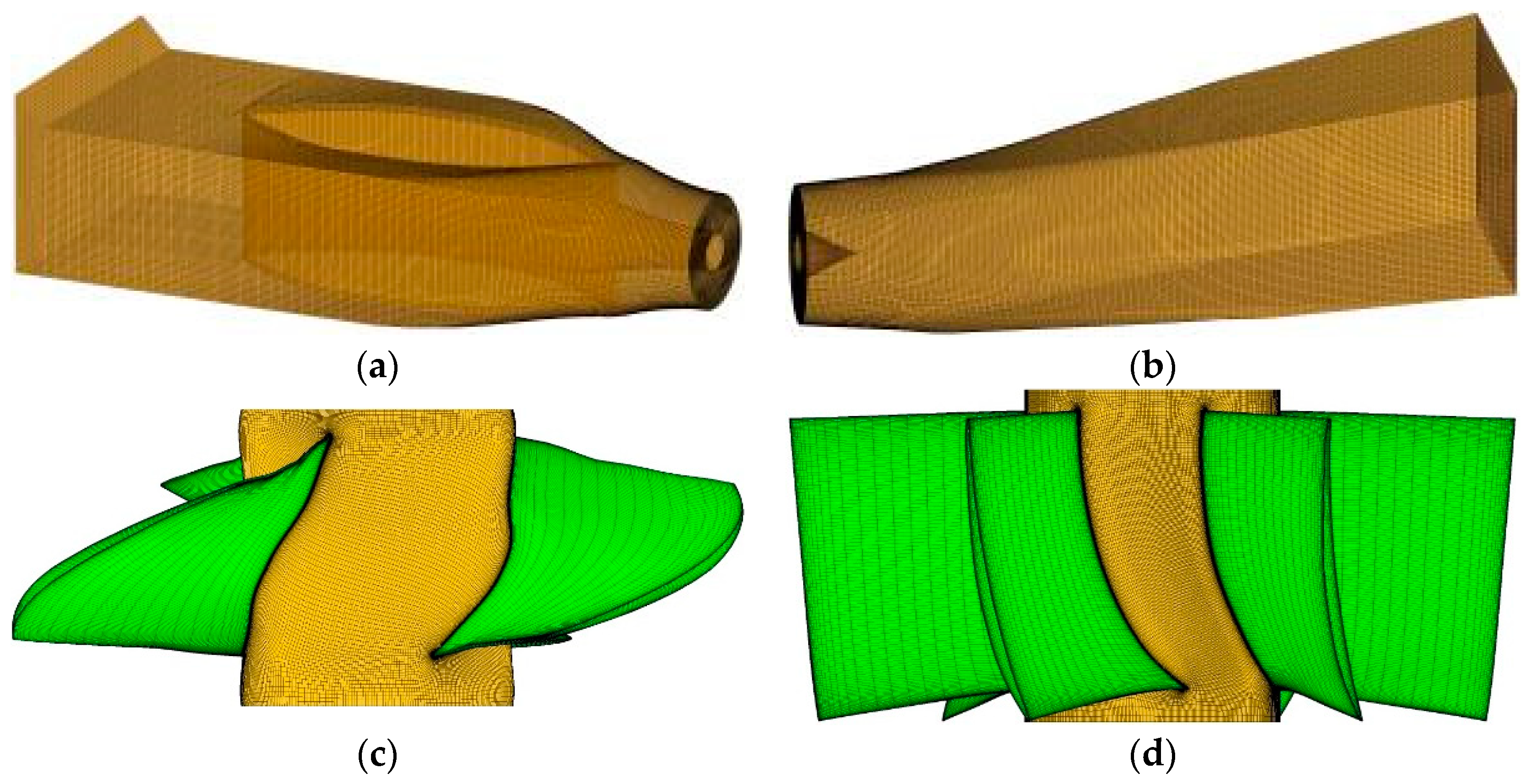
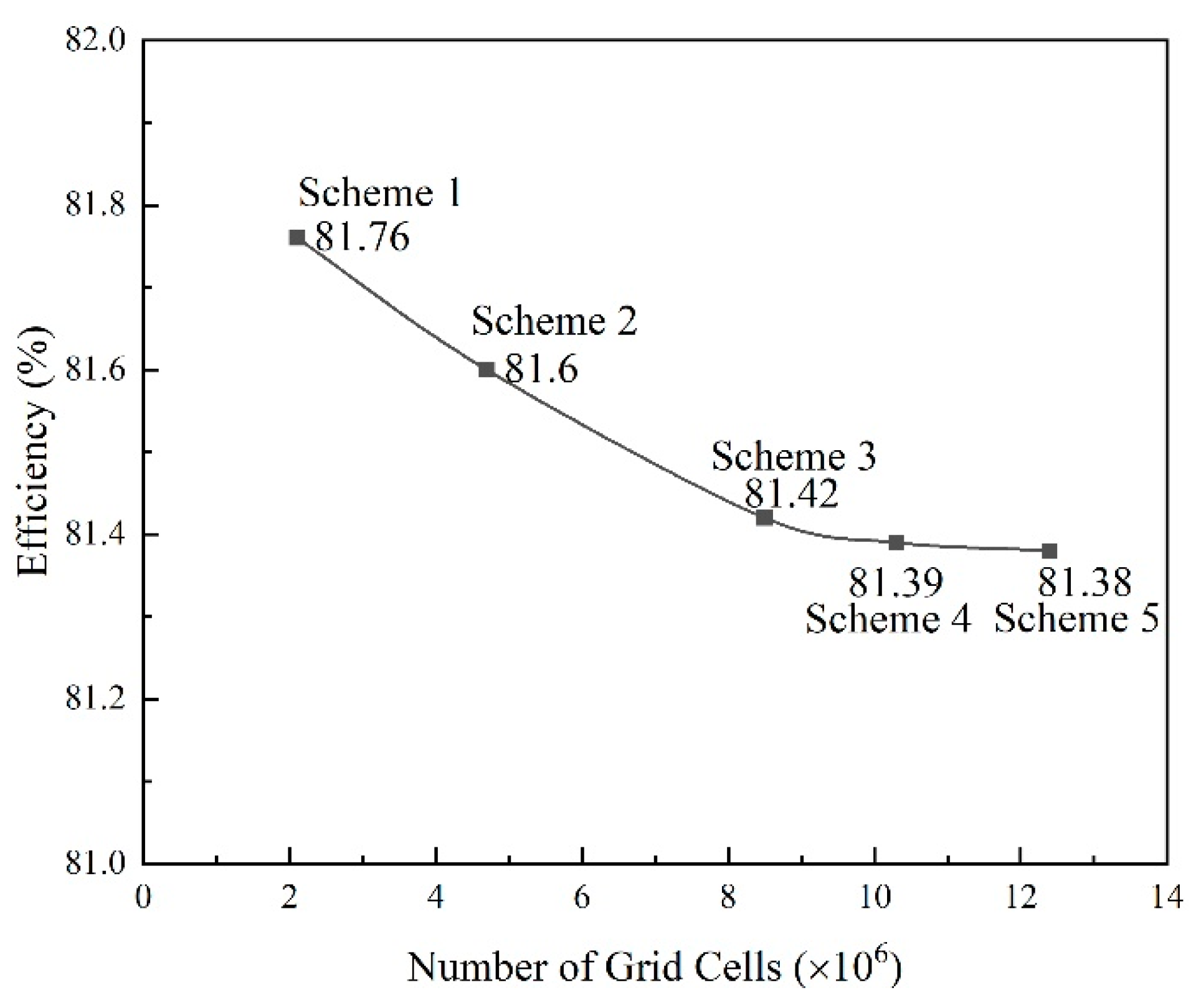
2.2. Grid Division and Scheme Selection

The mesh of different components of the STPD was generated by using the ICEM and ANSYS Turbogrid. The mesh of the different parts is shown in Figure 2.

To ensure that the calculation results were not influenced by the mesh, five schemes were compared. The number of grid cells for the five schemes was 2.1 million, 4.7 million, 8.5 million, 10.3 million, and 12.4 million. Figure 3 shows that the change in results between scheme 4 and scheme 5 is only 0.01%. Considering the computational resources, scheme 4 was initially chosen.

In order to ensure the convergence of the mesh, according to reference [42], the mesh convergence was verified by using the grid convergence index.

Table 1. The verification process.

Parameters	Values
N1, N2, N3	10.3 M, 4.7 M, 2.1 M
r21, r32	1.303, 1.318
Φ1, Φ2, Φ3	81.38%, 81.60%, 81.76%
p	2.28
${\Phi }_{ext}^{21}$, ${\Phi }_{ext}^{32}$	1.22, 1.21
$e_a^{21}$, $e_a^{32}$	0.30%, 0.17%
GCI21	0.45%
GCI32	0.24%

shows the verification process of the mesh convergence, and the results show that the convergence of scheme 4 meets the requirements.

The impeller was evenly divided into 10 subdomains, which along axial and radial directions were IA1~IA10 and IR1~IR10, as shown in Figure 4. In IR10, there was a tip clearance between the blade and shroud. According to previous studies, the flow in this region is complex, and the energy loss in this region accounts for a large part of the energy loss in the impeller. Therefore, in this study, schemes 3, 4, and 5 were chosen to conduct an independence analysis of the mesh in this region, and the energy loss in IR10 under the design flow rate condition was used as the control index. In these three schemes, the number of nodes in the tip clearance along the radial direction was 15, 22, and 31, respectively.

Table 2. Mesh independence analysis of the tip clearance.

Scheme	Number of Grid Cells/106	Number of Nodes in the Tip Clearance	Turbulent Entropy Production in IR10/W
3	8.5	15	330.1
4	10.3	22	338.7
5	12.4	31	340.6

shows the energy loss results under different numbers of nodes in the tip clearance region. The results show that the relative variation between scheme 4 and scheme 5 is only 0.56%; hence, scheme 4 could be used in the numerical simulation. The average Yplus values of the inlet passage, impeller, guide vanes, and outlet passages are 13.33, 8.61, 9.37, and 10.87, respectively. According to Refs. [35,43,44,45], the Yplus values of each part are in the range of 20~100. Hence, scheme 4 is a reasonable choice.

Overall, considering the grid independence, GCI, and the mesh independence of the tip clearance, scheme 4 satisfies all requirements, so it was used in the numerical simulation.

2.3. Boundary Conditions and Settings

The commercial software ANSYS CFX 19.2 [46] was applied to simulate the flow in the STPD. The inlet boundary condition was set to the total pressure with a value of 1 atm. The outlet boundary condition was set to the mass flow, and the flow range for this numerical simulation was 0.3~1.0 Q_d. All the solid wall surfaces were set to the no-slip wall conditions. In the steady and unsteady simulation, the interface between the stationary domains was set as “None”. In the steady simulation, the interface between the stationary and rotation domains was set as “Frozen Rotor”, while in the unsteady simulation the interface was set as “Transient Rotor Stator”. According to the previous studies [47], the time step is generally selected to be 3 degrees of impeller rotation, and the total time should be more than 6 cycles. Hence, total simulation time was set to 0.828 s, which is equivalent to 20 cycles. The time step was set to 3.45 × 10⁻⁴ s, which is equivalent to 3° of impeller rotation. The advection scheme was set as “Upwind”. The convergence standard was set as −10⁻⁴.

2.4. Entropy Production Method

According to the causes, entropy production can be divided into two categories in turbulent flow. The direction entropy production rate (DEPR) can be obtained by using Equation (13).

$$\begin{array}{l}{\dot{S}}_{\overline{D}}^{‴}=\frac{2\mu }{T}\left[{\left(\frac{\partial u_1}{\partial x_1}\right)}^2+{\left(\frac{\partial u_2}{\partial x_2}\right)}^2+{\left(\frac{\partial u_3}{\partial x_3}\right)}^2\right]\\ +\frac{\mu }{T}\left[{\left(\frac{\partial u_2}{\partial x_1}+\frac{\partial u_1}{\partial x_2}\right)}^2+{\left(\frac{\partial u_3}{\partial x_1}+\frac{\partial u_1}{\partial x_3}\right)}^2+{\left(\frac{\partial u_2}{\partial x_3}+\frac{\partial u_3}{\partial x_2}\right)}^2\right]\end{array}$$

(13)

The turbulent entropy production method rate (TEPR) can be obtained by using Equation (14) proposed by Mathieu [48]:

$${\dot{S}}_{D^{\prime }}^{‴}=\beta \frac{\rho \omega k}{T}$$

(14)

The direct entropy production (DEP) and turbulent entropy production (TEP) can be obtained by integration of DEPR and TEPR:

$$P_{\mathrm{S}\mathrm{D}}{=P}_{S\overline{D}}+P_{S{D}^{\prime }}={\int }_V{\dot{S}}_{\overline{D}}^{‴}dV·T+{\int }_V{\dot{S}}_{D^{\prime }}^{‴}dV·T$$

(15)

The entropy production in the wall region (EPW) can be obtained by using Equation (16):

$$P_{\mathrm{S}\mathrm{W}}={\int }_A\frac{\overline{\tau }·\overline{v}}{T}dA·T$$

(16)

The sum of the above three entropy production values is the energy loss in the STPD.

3. Model Test

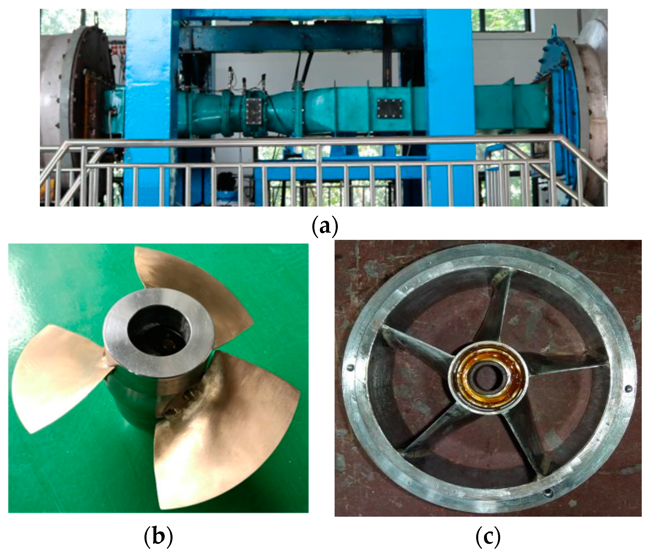
3.1. Test Equipment and Procedures

Pictures of the model test are shown in Figure 5. The measurement instruments and measurement uncertainties of the test rig are introduced in Ref. [7]. The model test was carried out strictly in accordance with IEC standards. In this study, the energy performance test was performed under the condition that no cavitation occurs, so cavitation was not considered in the numerical simulation.

3.2. Model Test Results

The results of the model test can be seen in Figure 6. When the flow rate is less than 0.46 Q_d and greater than 0.6 Q_d, the slope of the head curve is negative; however, when it is 0.46 Q_d~0.6 Q_d, the slope is positive. The shape of the head curve in this range is like a saddle, so this region can also be called the saddle-shaped region. According to Ref. [14], when the slope of the head curve begins to become positive, it indicates that the STPD has started to enter the stall condition. Hasmatuchi et al. [49] proposed that the flow rate condition corresponding to the lowest head in the saddle-shaped region can be regarded as a severe stall condition. Based on previous research, in this study the critical and severe stall conditions occur at flow rates of 0.6 Q_d and 0.46 Q_d, respectively.

4. Results and Discussion

4.1. Reliability Analysis of Numerical Simulation

The results of the numerical simulation and model test were comparatively analyzed. It can be found from Figure 7 that the variation trends of the curves obtained by the two methods are consistent. The maximum head and efficiency errors occur at 0.3 Q_d, with absolute errors of 0.48 m and 0.95% and relative errors of 4.97% and 3.23%. The maximum shaft power error occurs at a flow rate of 0.46 Q_d, and the absolute and relative errors are 0.74 kW and 2.54%, respectively. This is because the flow has high curvature in the pump under this condition. Although the turbulence model was corrected by the curvature correction method in this study, it is unable to simulate the mechanical loss; hence, some minor errors were inevitable.

In conclusion, the SST k-ω model, corrected by the curvature correction method, proves to be more effective in simulating the performance of the STPD. The relative error under each condition remains below 5%, indicating that the results of this study can be deemed reliable.

Figure 8 illustrates the energy loss in the STPD, revealing that TEP is the main contributor to the loss. In addition, the value of DEP is small and can be ignored under all operating conditions. It is evident that the energy loss in STPD increases as the stall condition worsens.

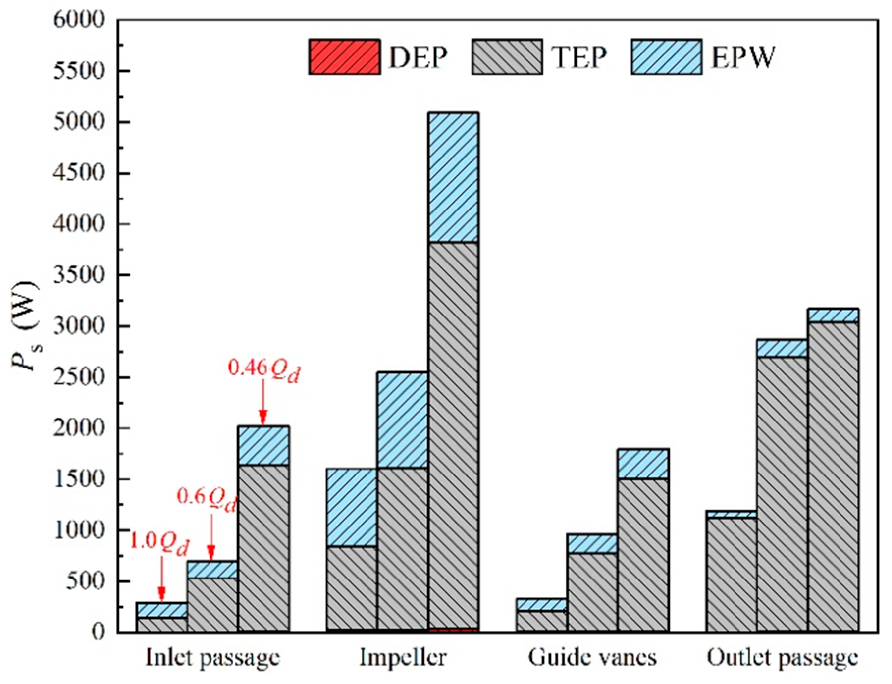
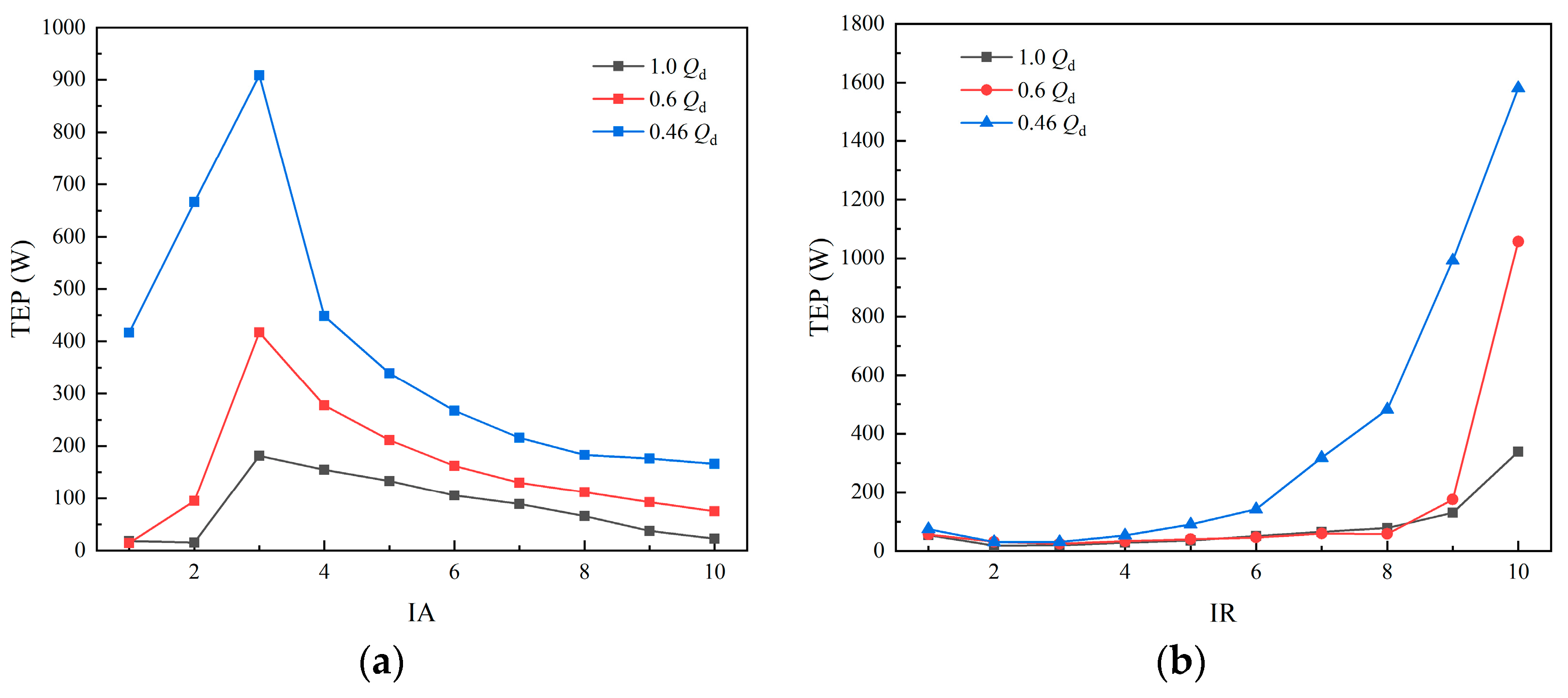
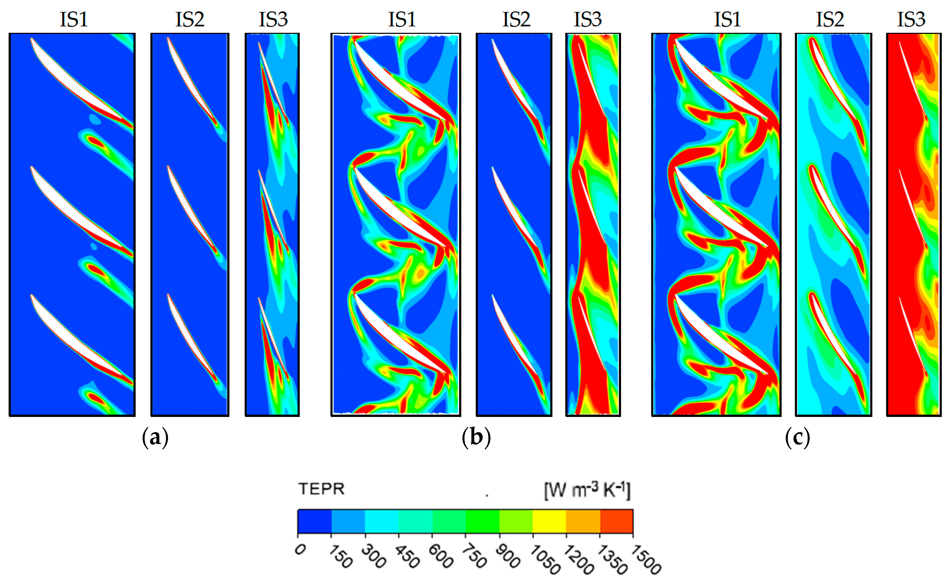
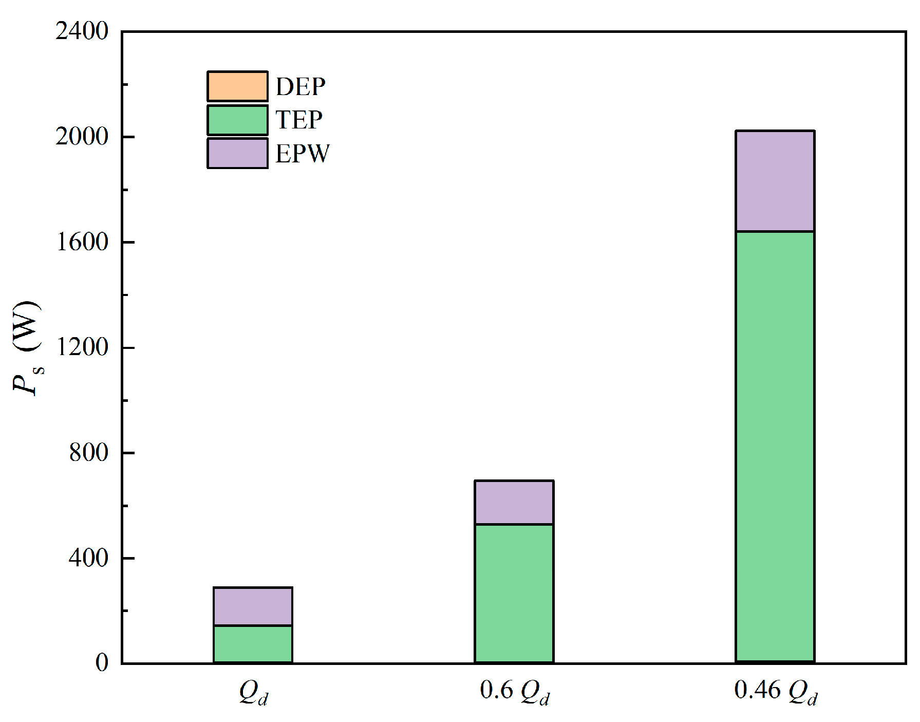
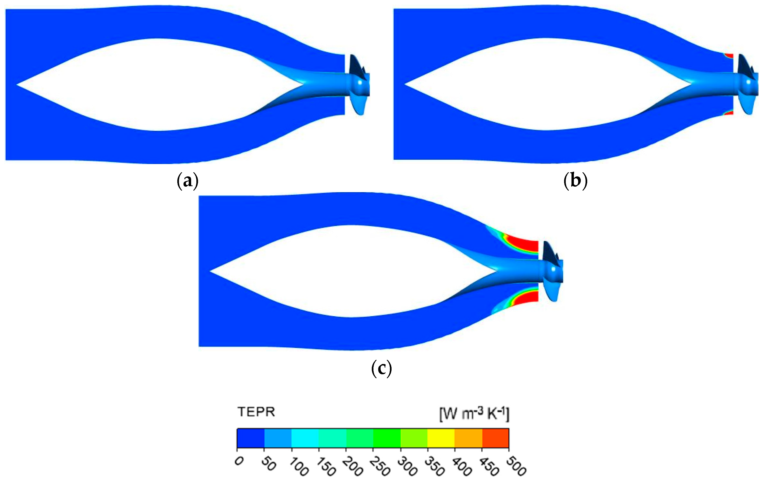
4.2. The Energy Loss Characteristics of Impeller and Guide Vanes

In this study, the design, critical stall, and severe stall conditions were selected for analysis. Figure 9 illustrates the energy loss in the impeller; the energy loss can be divided into DEP, TEP, and EPW. The proportions of the three types of entropy production under the design condition are 1.3%, 51.2%, and 47.5%, respectively; under the critical stall condition are 1.1%, 62.1%, and 36.8%, respectively; and under the severe stall condition are 0.7%, 74.4%, and 24.9%, respectively. It is obvious that the proportion of TEP is the highest at all operating conditions, which indicates that TEP is the main contributor to the loss. With the worsening of the stall, the TEP increases significantly. Under critical and severe stall conditions, the TEP is 1.93 and 4.61 times higher than under the design condition, respectively. In addition, both the DEP and EPW also increase with the worsening of the stall, but the growth rate is significantly lower than that of TEP. DEP exhibits especially low sensitivity to the change in operating conditions.

The TEP in the subdomains of the impeller is illustrated in Figure 10. The TEP reaches a peak at all operating conditions, and the peak value increases substantially with the worsening of the stall in IA3. The TEP in IA3 under critical and severe stall conditions is 2.3 and 5.02 times higher than that under the design condition, respectively. This is a result of the flow detachment in the leading edge under stall conditions [50]. The significant increase in TEP in IA1 and IA2 under the severe stall condition is also due to the flow separation’s even backflow. From IA4 to IA10, the TEP in each subdomain gradually decreases, and the TEP demonstrates an increasing trend as the flow rate decreases.

Along the radial direction, the TEP value is maximum in IR10 and increases with the worsening of the stall. The volume of IR10 accounts for only 12.28% of the total volume of the impeller, but the TEP in this region is beyond 41% of the total TEP. This is because there is a tip leakage vortex (TLV) in this region, and the TLV extends farther as the flow rate becomes lower [51]. Moreover, the TEP value in IR1 is higher than the adjacent subdomain, which is caused by the influence of the wall effect near the hub region.

Three typical sections were selected for the visualization of the loss. The Span values of the three sections were 0.03, 0.5, and 0.97, respectively, and named IS1~IS3. The distribution of TEPR is illustrated in Figure 11, and from left to right, IS1~IS3. The high-TEPR regions are mainly in the hub and shroud regions. Near the hub region (IS1), a high-TEPR region exists in the passage as well as the tail of the blade under three conditions, which are caused by the hub vortex and the flow separation in the tail of the blade. Moreover, the high-TEPR region expands as the flow rate becomes smaller. Under critical and stall conditions, there is a horseshoe vortex at the leading edge of the blade, so the TEPR in this region is also high, and as the stall worsens, the range of the horseshoe vortex increases, and thus the range of the high-TEPR region also increases. In the middle passage of the impeller (IS2), the flow pattern is stable. Therefore, under the design and critical stall conditions, there are only small regions of high TEPR at the trailing edge. However, under the severe stall condition, the flow in the impeller deteriorates further, and a cross-passage vortex appears in the impeller, leading to a significant increase in TEPR. Near the shroud region (IS3), as the stall becomes more severe, the range of the TLV and the backflow at the leading edge increases, leading to an increase in the high-TEPR region. Under the severe stall condition, the high-TEPR region continues to increase and occupies almost the entire blade passage.

The energy loss in the guide vanes is illustrated in Figure 12. TEP is the main contributor to the loss, and its proportion increases with decreasing flow rate. The TEP accounts for 60.83% of the total entropy production under design conditions, while under critical and severe stall conditions, the TEP accounts for 79.27% and 83.13%, respectively. Under critical and severe stall conditions, the TEP is 2.92 and 5.54 times higher than under design conditions, respectively.

Similarly, three typical sections in the guide vanes were also selected along the radial direction for loss visualization. The Span values of the three sections were 0.03, 0.5, and 0.97, respectively, and named GS1~GS3. The TEPR distribution in the guide vanes is shown in Figure 13, and from left to right, GS1~GS3. Near the hub region (GS1), the high-TEPR region exists at the inlet of the pressure surface of the guide vanes under the design condition, while as the flow rate decreases, the region gradually moves to the guide vane outlet and extends farther. In the middle passage of the impeller (GS2), there is no high-TEPR region under the design condition because the flow pattern is stable. Under stall conditions, a high-TEPR region occurs on the suction surface. This is because of the inconsistency between the flow angle and the installation angle of the guide vanes resulting in a flow separation vortex. As the stall deteriorates, the flow separation vortex intensifies, and the range of the high-TEPR region increases accordingly. Near the shroud region (GS3), as the stall phenomenon worsens, the influence of the impeller blade wake vortex on the internal flow in the guide vanes becomes more significant, resulting in an increasing of TEPR, especially at the inlet part.

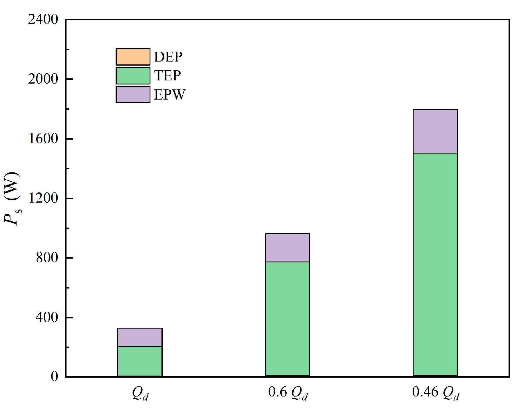
4.3. The Energy Loss Characteristics of Inlet Passage

The inlet passage is positioned upstream of the impeller and is used to guide the water flow evenly and smoothly into the impeller and provide good working conditions for the impeller. The energy loss under different conditions is shown in Figure 14. Under design conditions, the loss is small, and the main sources of energy loss are TEP and EPW, which account for 47.9% and 50.7%, respectively, while DEP is negligible. Under critical stall conditions, the TEP is 3.79 times higher, and the percentage of TEP in the energy loss is increased to 75.7%. The increasing of TEP is more dramatic under severe stall conditions; the TEP is 11.83 times higher, and the proportion of TEP is further increased to 80.7%. This is caused by the expansion of the backflow range in the impeller.

In order to further reveal the impact of the backflow from the impeller on the flow pattern in the inlet passage under stall conditions, a dimensionless variable W was used in this study. When W < 0, it means that there is a backflow, and when the W is closer to 1, it indicates that the axial velocity is dominant. The expression is

$$W=\frac{\overline{V_a}}{\left|\overline{V}\right|}$$

(17)

where $\overline{V_a}$ and $\overline{V}$ are the time-averaged axial and resultant velocities.

Figure 15 shows the distribution of the W value in the horizontal section of the inlet passage. Since the backflow area is located in the rear part and there is no backflow in the front part of the inlet passage, for convenience of observation the distribution of the W value in the front part is not shown. As shown in Figure 15, there is no backflow in the inlet passage under design conditions. When stall begins, a small area of backflow exists near the outlet section. Under severe stall conditions, the range of backflow in the inlet passage expands significantly due to the worsening of the flow separation in the impeller. Figure 16 shows the distribution of TEPR in the inlet passage. The location of the high-TEPR area coincides with the backflow, which suggests that the notable increase in energy loss under stall conditions is primarily caused by the backflow from the impeller.

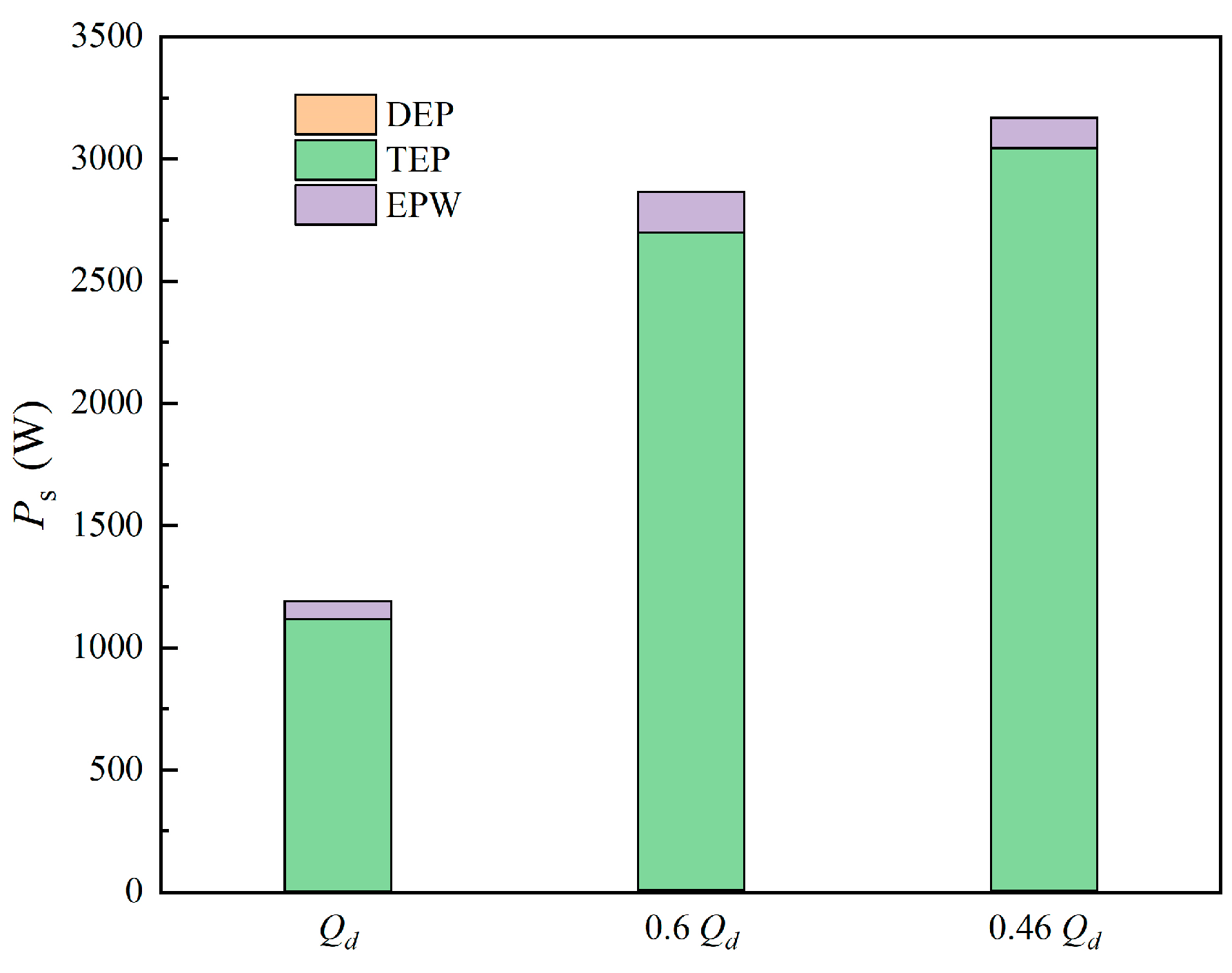
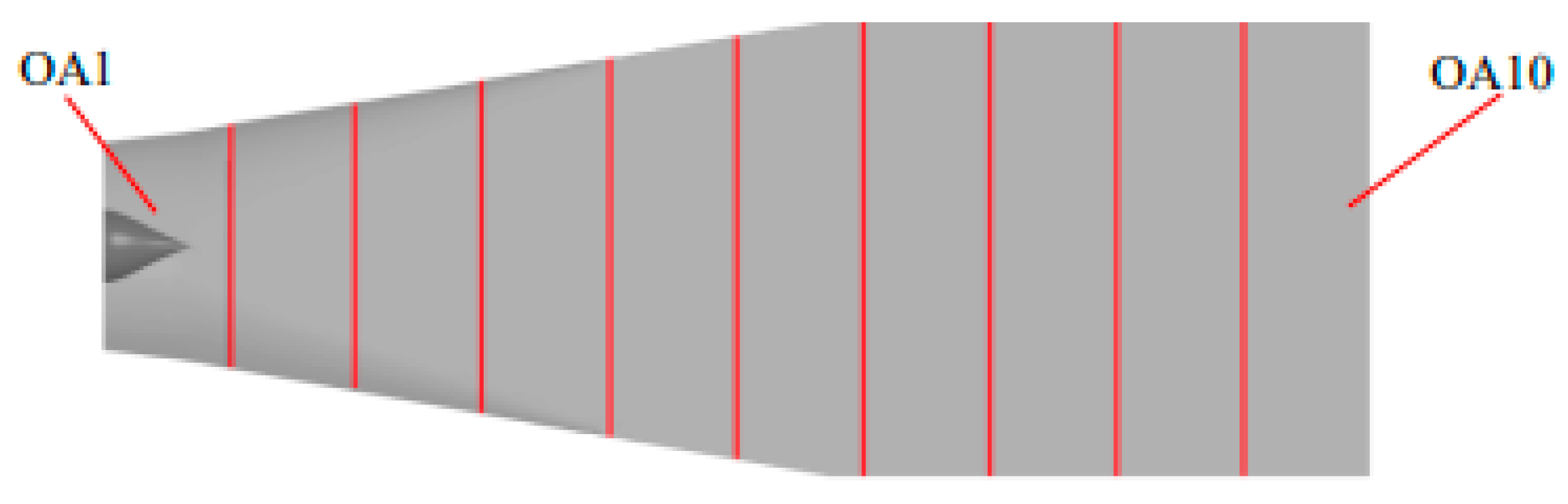
4.4. The Energy Loss Characteristics of Outlet Passage

Figure 17 shows the energy loss in the outlet passage. Consistent with other parts of the STPD, TEP is also the main source of loss, and the proportion exceeds 90% under the three operating conditions. Under critical and severe stall conditions, the TEP is 2.42 and 2.73 times higher than under the design condition, respectively. The adjustment ability of the guide vanes is weakened under the stall condition, so the circulation of the flow entering the outlet passage is large. Moreover, the flow in the outlet passage is also disturbed by the wake flow from the guide vanes.

Figure 18 shows the subdomains of the outlet passage along the axis, named OA1~OA10 from inlet to outlet. Figure 19 shows the TEP in the subdomains. Under the design condition, the TEP in each subdomain is relatively uniform, with a small increase in TEP from OA1 to OA4 as the volume increases. After OA4, the diffusion of the flow is basically completed, and the flow velocity and circulation begin to decrease; hence, the TEP gradually drops. Under critical and severe stall conditions, the energy loss is mainly concentrated in OA1, which accounts for only 4.3% of the total volume, while the TEP proportion in OA1 is 67.5% under critical conditions and even up to 76.9% under severe stall conditions. This is primarily attributed to the large velocity and circulation of the flow in OA1 and the vortex at the tail of the guide vanes.

To further explore the distribution pattern of TEPR, several typical sections were used to visualize and analyze the energy loss; the locations and names of these sections are shown in Figure 20. OS1 is the horizontal section, and the typical sections distributed along the axial direction are OS2~OS7, where OS2 is the inlet of the outlet passage, and the distances of OS3~OS7 from the inlet are 0.33, 0.67, 1.0, 1.33, and 2.0 times the impeller diameter, respectively. According to Figure 21, it is obvious that the energy loss is mostly concentrated near the inlet, and the TEPR in this region increases with the severity of the stall, which is consistent with the pattern in Figure 19. There are six high-TEPR regions in OS2. The number of high-TEPR regions corresponds to the number of guide vanes, and the intensity increases with decreasing flow. In addition, the higher flow velocity near the outer wall is a result of the centrifugal force, which leads to a higher TEPR in that region.

5. Conclusions

In this study, an STPD was used as the research object, and the energy loss characteristics under the design condition and two stall conditions were compared and analyzed. Finally, the various laws of energy loss characteristics of each part of the STPD under operating conditions were revealed. The main conclusions are as follows:

1. The SST k-ω turbulence model with curvature correction can effectively predict the hydraulic performance and flow of the STPD, especially under stall conditions. For the STPD, the stall starts to occur when the flow rate is 0.6 Q_d. The critical and sever stall conditions of the STPD are 0.6 Q_d and 0.46 Q_d, respectively.

2. Under all conditions, TEP is the main loss source in all parts of the STPD, and it increases very significantly with the worsening of stall. Compared with the design conditions, under critical and severe stall conditions, the TEP in the impeller is 1.93 and 4.61 times higher; the TEP in the guide vanes is 2.92 and 5.54 times higher; the TEP in the inlet passage is 3.79 and 11.83 times higher; and the TEP in the outlet passage is 2.42 and 2.73 times higher, respectively.

3. The high-TEPR regions in the impeller are mainly concentrated in the area near the shroud and hub due to the influence of the hub vortex and the TLV, and the TEPR in the middle passage of the impeller increases significantly under severe stall conditions. In addition, the extent of the high-TEPR region in the inlet section of the impeller continues to increase with the worsening of stall. Influenced by the flow from the impeller and the separation vortex in the guide vanes, the high-TEPR regions in the guide vanes are mainly concentrated near the shroud and the suction surface of the blade, and the TEPR in the inlet section of the guide vanes also increases significantly with the deterioration of stall.

4. By the influence of the backflow from the impeller, the high TEPR in the inlet passage is distributed near the outlet segment, which is basically the same as the location of the backflow area. The majority of the energy loss in the outlet passage is concentrated in the entrance part, primarily due to the presence of the wake flow of the guide vanes.

References

1. Shi, L.J.; Chai, Y.; Wang, L.; Xu, T.; Jiang, Y.; Xing, J.; Yan, B.; Chen, Y.; Han, Y. Numerical simulation and model test of the influence of guide vane angle on the performance of axial flow pump. Phys. Fluids 2023, 35, 015129. [Google Scholar] [CrossRef]
2. Gopal, C.; Mohanraj, M.; Chandramohan, P.; Chandrasekar, P. Renewable energy source water pumping systems-A literature review. Renew. Sustain. Energy Rev. 2013, 25, 351–370. [Google Scholar] [CrossRef]
3. Ji, D.T.; Lu, W.G.; Lu, L.G.; Xu, L.; Liu, J.; Shi, W.; Huang, G.H. Study on the Comparison of the Hydraulic Performance and Pressure Pulsation Characteristics of a Shaft Front-Positioned and a Shaft Rear-Positioned Tubular Pump Devices. J. Mar. Sci. Eng. 2021, 10, 8. [Google Scholar] [CrossRef]
4. Luo, C.; Du, K.; Qi, W.J.; Cheng, L.; Huang, X.B.; Lu, J.X. Investigation on the Effect of the Shaft Transition Form on the Inflow Pattern and Hydrodynamic Characteristics of the Pre-Shaft Tubular Pump Device. Front. Energy Res. 2022, 10, 955492. [Google Scholar] [CrossRef]
5. Emmons, H.W.; Pearson, C.E.; Grant, H.P. Compressor surge and stall propagation. Trans. ASME 1955, 2, 455–469. [Google Scholar] [CrossRef]
6. Sinha, M.; Pinarbasi, A.; Katz, J. The flow structure during onset and developed states of rotating stall within a vaned diffuser of a centrifugal pump. J. Fluids Eng. 2001, 123, 490–499. [Google Scholar] [CrossRef] [Green Version]
7. Ji, D.T.; Lu, W.G.; Lu, L.G.; Xu, L.; Liu, J.; Shi, W.; Zhu, Y. Comparison of Saddle-Shaped Region of Head-Flow Curve between Axial-Flow Pump and Its Corresponding Axial-Flow Pump Device. Shock. Vib. 2021, 2021, 1–17. [Google Scholar] [CrossRef]
8. Day, I.J. Stall, Surge, and 75 Years of Research. J. Turbomach. 2016, 138, 011001. [Google Scholar] [CrossRef]
9. Pedersen, N.; Larsen, P.S.; Jacobsen, C.B. Flow in a centrifugal pump impeller at design and off-design conditions—Part I: Particle image velocimetry (PIV) and laser Doppler velocimetry (LDV) measurements. J. Fluids Eng. 2003, 125, 61–72. [Google Scholar] [CrossRef]
10. Miyabe, M.; Maeda, H.; Umeki, I.; Jittani, Y. Unstable Head-Flow Characteristic Generation Mechanism of a Low Specific Speed Mixed Flow Pump. J. Therm. Sci. 2006, 15, 115. [Google Scholar] [CrossRef]
11. Geng, W.; Liu, C.; Tang, F. 3D-PIV measurements of flow fields at exit to impeller of an axial flow pump. J. Hohai Univ. Nat. Sci. 2010, 38, 516–521. [Google Scholar]
12. Yao, Z.; Wang, F.; Qu, L.; Xiao, R.; He, C.; Wang, M. Experimental Investigation of Time-Frequency Characteristics of Pressure Fluctuations in a Double-Suction Centrifugal Pump. J. Fluids Eng. 2011, 133, 101303. [Google Scholar] [CrossRef]
13. Wu, D.; Ren, Y.; Mou, J.; Gu, Y. Investigation of the correlation between noise & vibration characteristics and unsteady flow in a circulator pump. J. Mech. Sci. Technol. 2017, 31, 2155–2166. [Google Scholar] [CrossRef]
14. Goltz, I.; Kosyna, G.; Stark, U.; Saathoff, H.; Bross, S. Stall inception phenomena in a single-stage axial-flow pump. Proc. Inst. Mech. Eng. Part A J. Power Energy 2003, 217, 471–479. [Google Scholar] [CrossRef]
15. Yuan, Z.; Yujie, C.; Rui, Z.; Xinfeng, G.; Guopeng, L.; Aoran, S. Analysis on Unsteady Stall Flow Characteristics of Axial-flow Pump. Trans. Chin. Soc. Agric. Mach. 2017, 48, 127–135. [Google Scholar]
16. Mu, T.; Zhang, R.; Xu, H.; Zheng, Y.; Fei, Z.; Li, J. Study on improvement of hydraulic performance and internal flow pattern of the axial flow pump by groove flow control technology. Renew. Energy 2020, 160, 756–769. [Google Scholar] [CrossRef]
17. Ji, L.L.; Li, W.; Shi, W.D. Influence of tip leakage flow and inlet distortion flow on a mixed-flow pump with different tip clearances within the stall condition. Proc. Inst. Mech. Eng. Part A J. Power Energy 2020, 234, 433–453. [Google Scholar] [CrossRef]
18. Toyokura, T. Studies on the Characteristics of Axial-Flow pumps: Part 1, General Tendencies of the Characteristics of Pumps. Bull. JSME 1961, 14, 287–293. [Google Scholar] [CrossRef]
19. Zierke, W.C.; Straka, W.A.; Taylor, P.D. An Experimental Investigation of the Flow Through an Axial-Flow Pump. J. Fluids Eng. 1995, 117, 485–490. [Google Scholar] [CrossRef]
20. Benra, F.K.; Dohmen, H.J. Unsteady Three-Dimensional Flow Phenomena in an Axial Flow Pump at Different Operating Points. In ASME 2008 Fluids Engineering Division Summer Meeting Collocated with the Heat Transfer, Energy Sustainability, and 3rd Energy Nanotechnology Conferences; American Society of Mechanical Engineers: New York, NY, USA, 2008; pp. 277–283. [Google Scholar]
21. Farrell, K.J.; Billet, M.L. A correlation of leakage vortex cavitation in axial-flow pumps. J. Fluids Eng. 1994, 3, 551–557. [Google Scholar] [CrossRef]
22. Canbaz, O.; Yucel, N.; Albayrak, K. Experimental Investigation of Unsteady Flow in a Vertical Shaft Axial Flow Pump. J. Polytech. 2022. [Google Scholar] [CrossRef]
23. Kan, K.; Zheng, Y.; Chen, Y.; Xie, Z.; Yang, G.; Yang, C. Numerical study on the internal flow characteristics of an axial-flow pump under stall conditions. J. Mech. Sci. Technol. 2018, 32, 4683–4695. [Google Scholar] [CrossRef]
24. Kock, F.; Herwig, H. Local entropy production in turbulent shear flows: A high-Reynolds number model with wall functions. Int. J. Heat Mass. Trans. 2004, 47, 2205–2215. [Google Scholar] [CrossRef]
25. Herwig, H.; Kock, F. Local Entropy Production in Turbulent Shear Flows: A Tool for Evaluating Heat Transfer Performance. J. Therm. Sci. 2006, 15, 159–167. [Google Scholar] [CrossRef]
26. McEligot, D.M.; Nolan, K.P.; Walsh, E.J.; Laurien, E. Effects of pressure gradients on entropy generation in the viscous layers of turbulent wall flows. Int. J. Heat Mass. Trans. 2008, 51, 1104–1114. [Google Scholar] [CrossRef]
27. McEligot, D.M.; Brodkey, R.S.; Eckelmann, H. Laterally converging duct flows. Part 4. Temporal behaviour in the viscous layer. J. Fluids Mech. 2009, 634, 433–461. [Google Scholar] [CrossRef]
28. Schmandt, B.; Herwig, H. Internal Flow Losses: A Fresh Look at Old Concepts. J. Fluids Eng. 2011, 133, 051201. [Google Scholar] [CrossRef]
29. Herwig, H.; Gloss, D.; Wenterodt, T. A new approach to understanding and modelling the influence of wall roughness on friction factors for pipe and channel flows. J. Fluids Mech. 2008, 613, 35–53. [Google Scholar] [CrossRef]
30. Gong, R.; Wang, H.; Chen, L.; Li, D.; Zhang, H.; Wei, X. Application of entropy production theory to hydro-turbine hydraulic analysis. Sci. China Technol. Sci. 2013, 56, 1636–1643. [Google Scholar] [CrossRef]
31. Ghorani, M.M.; Haghighi, M.H.S.; Maleki, A.; Riasi, A. A numerical study on mechanisms of energy dissipation in a pump as turbine (PAT) using entropy generation theory. Renew. Energy 2020, 162, 1036–1053. [Google Scholar] [CrossRef]
32. Osman, M.K.; Wang, W.; Yuan, J.; Zhao, J.; Wang, Y.; Liu, J. Flow loss analysis of a two-stage axially split centrifugal pump with double inlet under different channel designs. Proc. Inst. Mech. Eng. Part C J. Mech. Eng. Sci. 2019, 233, 5316–5328. [Google Scholar] [CrossRef]
33. Zhou, L.; Hang, J.; Bai, L.; Krzemianowski, Z.; El-Emam, M.A.; Yasser, E.; Agarwal, R. Application of entropy production theory for energy losses and other investigation in pumps and turbines: A review. Appl. Energy 2022, 318, 119211. [Google Scholar] [CrossRef]
34. Ren, Y.; Zhu, Z.; Wu, D.; Li, X. Influence of Guide Ring on Energy Loss in a Multistage Centrifugal Pump. J. Fluids Eng. 2018, 141, 061302. [Google Scholar] [CrossRef]
35. Sun, L.; Pan, Q.; Zhang, D.; Zhao, R.; van Esch, B.P.M.B. Numerical study of the energy loss in the bulb tubular pump system focusing on the off-design conditions based on combined energy analysis methods. Energy 2022, 258, 124794. [Google Scholar] [CrossRef]
36. Menter, F.R. Review of the shear-stress transport turbulence model experience from an industrial perspective. Int. J. Comput. Fluid Dyn. 2009, 23, 305–316. [Google Scholar] [CrossRef]
37. Kim, Y.; Heo, M.; Shim, H.; Lee, B.; Kim, D.; Kim, K. Hydrodynamic Optimization for Design of a Submersible Axial-Flow Pump with a Swept Impeller. Energies 2020, 13, 3053. [Google Scholar] [CrossRef]
38. Li, W.; Ji, L.; Li, E.; Shi, W.; Agarwal, R.; Zhou, L. Numerical investigation of energy loss mechanism of mixed-flow pump under stall condition. Renew. Energy 2021, 167, 740–760. [Google Scholar] [CrossRef]
39. Smirnov, P.E.; Menter, F.R. Sensitization of the SST Turbulence Model to Rotation and Curvature by Applying the Spalart-Shur Correction Term. J. Turbomach. 2009, 131, 041010. [Google Scholar] [CrossRef]
40. Huang, X.; Yang, W.; Li, Y.; Qiu, B.; Guo, Q.; Liu, Z. Review on the sensitization of turbulence models to rotation/curvature and the application to rotating machinery. Appl. Math. Comput. 2019, 341, 46–69. [Google Scholar] [CrossRef]
41. Spalart, P.R.; Shur, M. On the Sensitization of Turbulence Models to Rotation and Curvature. Aerosp. Sci. Technol. 1997, 5, 297–302. [Google Scholar] [CrossRef]
42. Roache, P.J. Conservatism of the grid convergence index in finite volume computations on steady-state fluid flow and heat transfer. J. Fluids Eng. 2003, 125, 731–732. [Google Scholar] [CrossRef]
43. Meng, F.; Li, Y.J. Energy characteristics of a bidirectional axial-flow pump with two impeller airfoils based on entropy production analysis. Entropy 2022, 24, 962. [Google Scholar] [CrossRef] [PubMed]
44. Hou, H.C.; Zhang, Y.X.; Li, Z.L. A numerical research on energy loss evaluation in a centrifugal pump system based on local entropy production method. Therm. Sci. 2017, 21, 1287–1299. [Google Scholar] [CrossRef]
45. Zhang, H.Y.; Meng, F.; Cao, L.; Li, Y.J.; Wang, X.K. The Influence of a Pumping Chamber on Hydraulic Losses in a Mixed-Flow Pump. Processes 2022, 10, 407. [Google Scholar] [CrossRef]
46. ANSYS Inc. ANSYS CFX-Solver Theory Guide; ANSYS Inc.: Canonsburg, PA, USA, 2018. [Google Scholar]
47. Wang, F.J. Analysis Method of Flow in Pumps and Pumping Stations; China Water and Power Press: Beijing, China, 2020. [Google Scholar]
48. Mathieu, J.; Scott, J. An Introduction to Turbulent Flow; Cambridge University Press: Cambridge, UK, 2000. [Google Scholar]
49. Hasmatuchi, V.; Farhat, M.; Roth, S.; Botero, F.; Avellan, F. Experimental Evidence of Rotating Stall in a Pump-Turbine at Off-Design Conditions in Generating Mode. J. Fluids Eng. 2011, 133, 051104. [Google Scholar] [CrossRef]
50. Yang, H.; Sun, D.D.; Tang, F.P.; Zhang, X.F. Experiment research on inlet flow field for axial-flow pump at unsteady operating condition. J. Drain. Irrig. Mach. 2011, 29, 406–410. [Google Scholar]
51. Zhang, D.S.; Shi, W.D.; Pan, D.Z.; Dubuisson, M. Numerical and Experimental Investigation of Tip Leakage Vortex Cavitation Patterns and Mechanisms in an Axial Flow Pump. J. Fluids Eng. 2015, 137, 121103. [Google Scholar] [CrossRef]
Figure 1. Model of STPD.
Jmse 11 01512 g001
Figure 2. Grid diagram of STPD: (a) inlet passage; (b) outlet passage; (c) impeller; (d) guide vanes.
Jmse 11 01512 g002
Figure 3. Grid independence analysis.
Jmse 11 01512 g003
Figure 4. Division diagram of impeller: (a) axial direction; (b) radial direction.
Jmse 11 01512 g004
Figure 5. Pictures of the model test: (a) pump device; (b) impeller; (c) guide vanes.
Jmse 11 01512 g005
Figure 6. The results of the model test.
Jmse 11 01512 g006
Figure 7. Comparison of the numerical simulation and model test.
Jmse 11 01512 g007
Figure 8. The energy loss in STPD.
Jmse 11 01512 g008
Figure 9. The energy loss in impeller.
Jmse 11 01512 g009
Figure 10. The TEP in subdomains of impeller: (a) axially; (b) radially.
Jmse 11 01512 g010
Figure 11. The distribution of TEPR in impeller: (a) Q = 1.0 Qd; (b) Q = 0.6 Qd; (c) Q = 0.46 Qd.
Jmse 11 01512 g011
Figure 12. The energy loss in guide vanes.
Jmse 11 01512 g012
Figure 13. The distribution of TEPR in guide vanes: (a) Q = 1.0 Qd; (b) Q = 0.6 Qd; (c) Q = 0.46 Qd.
Jmse 11 01512 g013
Figure 14. The energy loss in inlet passage.
Jmse 11 01512 g014
Figure 15. The distribution of W: (a) Q = 1.0 Qd; (b) Q = 0.6 Qd; (c) Q = 0.46 Qd.
Jmse 11 01512 g015
Figure 16. The distribution of TEPR in inlet passage: (a) Q = 1.0 Qd; (b) Q = 0.6 Qd; (c) Q = 0.46 Qd.
Jmse 11 01512 g016
Figure 17. The energy loss in outlet passage.
Jmse 11 01512 g017
Figure 18. The subdomains of outlet passage.
Jmse 11 01512 g018
Figure 19. The TEP in subdomains of outlet passage.
Jmse 11 01512 g019
Figure 20. The locations and names of sections.
Jmse 11 01512 g020
Figure 21. The distribution of TEPR in outlet passage: (a) Q = 1.0 Qd; (b) Q = 0.6 Qd; (c) Q = 0.46 Qd.
Jmse 11 01512 g021aJmse 11 01512 g021b