Fault Diagnosis of Marine Diesel Engines under Partial Set and Cross Working Conditions Based on Transfer Learning

Abstract

The development of intelligent ships has an urgent demand for intelligent fault diagnosis technology. The working conditions and fault modes of high-power marine diesel engines gradually tend to be diversified and complicated, and the problems of reliability and safety are becoming more and more prominent. There are a lot of working condition data that lack fault labels, and the fault modes are asymmetric among different working conditions, so it is urgent to study effective fault diagnosis methods. Taking a marine diesel engine as the case validation object, we set up cross-condition and partial set fault diagnosis scenarios, proposed transferring knowledge from the source condition to the target condition for the problem of the lack of fault labels in the target condition, and designed a multi-scale and multi-view domain adversarial network (MMDAN) method for experimental validation using 6S50MC-C7 marine diesel engine system operation data. According to the experimental results, the average diagnostic accuracy of this method reached 96.58%, with a short processing time. Furthermore, it exhibits superior diagnostic performance compared to other transfer learning models in the cross-condition partial set transfer task. Additionally, the method proposed in this paper also offers a new approach and reference for the intelligent diagnosis of other equipment in ships.

1. Introduction

With the advancement in marine equipment automation and the increasing complexity of machinery, modern marine systems are moving towards expansion, reduced human intervention, and enhanced intelligence. Consequently, the demand for reliability in marine machinery and equipment is also on the rise. Diesel engines have long been used as power devices in the maritime industry, and their reliability is crucial to the safe and efficient operation of vessels. However, due to the prolonged exposure to high temperatures and pressures in their operational environment, diesel engines inevitably experience performance degradation and even failures. Therefore, to ensure navigation safety and minimize economic losses, it is necessary to conduct real-time performance monitoring and fault diagnosis. By contrast with traditional fault monitoring methods such as monitoring and alarms or manual inspections, intelligent fault monitoring methods can effectively and accurately handle large amounts of collected data, providing more reliable diagnostic results by reducing human intervention in fault monitoring. Indeed, data-driven intelligent fault diagnostic methods have emerged as a promising research topic in the maritime industry [1]. Unlike model-based fault diagnostic techniques, this approach does not require a significant amount of prior knowledge. Instead, it utilizes abundant real-time measurement data to construct fault models for predicting the health condition of diesel engines. Machine learning and deep learning technologies have made remarkable achievements in intelligent fault diagnosis for machinery as branches of data-driven methodologies. They can automatically learn useful information and features from historical monitoring data. Lazakis et al. [2] used an artificial neural network (ANN) model to predict the condition of marine mechanical systems. Zeng et al. [3] proposed a defense strategy for detecting and mitigating False Data Injection Attacks (FDIA) in ship DC microgrids. They employed an Artificial Neural Network (ANN) model for identifying and restoring corrupted data. The experimental results demonstrated the effectiveness of their method in detecting and mitigating FDIA, with errors less than 0.5 V. Qi et al. [4] proposed a deep learning model-based cabin auxiliary device detector, and the experimental results verified the effectiveness of the model. Wang et al. [5] introduced a stochastic convolutional neural network (CNN) structure in their work addressing the health monitoring of marine diesel engines. Their objective was to utilize convolutional computations and pooling operations within the CNN architecture to automatically extract discerning features from vibration signals. Han et al. [6] introduced CNN for detecting and isolating propeller faults in dynamically positioned marine vessels. Kim et al. [7] utilized a one-dimensional CNN model to analyze the vibration data of ship auxiliary equipment for fault diagnosis purposes. Ftoutou et al. [8] used an unsupervised fuzzy clustering approach for the time–frequency signal analysis of diesel engines, and the algorithm was experimentally proved to have a high fault detection rate. Diez Olivan et al. [9] put forward a comprehensive evaluation framework aimed at fault diagnosis for various states. This framework incorporated outlier detection and state characterization utilizing the K-means clustering algorithm. Additionally, fuzzy models of distances were employed for pattern recognition to accomplish fault diagnosis.

The above literature shows that both machine learning and deep learning have achieved good results in intelligent fault diagnosis methods for machinery. However, their ideal and assumed application scenarios present the following characteristics: (1) The samples in the training dataset (source domain) should have the same distribution as the samples in the testing dataset (target domain); (2) During the training phase, there are a large amount of labeled data available. However, due to the continuous operating conditions and dynamic working environment, the above assumptions are not satisfied in real industrial scenarios [10,11]. Undeniably, variations in distribution can result in the suboptimal performance of a model trained under certain conditions when applied to different conditions [12].

Transfer learning presents a promising paradigm for harnessing the acquired knowledge from annotated data in the source domain, thereby enabling the identification of the health status of unannotated data in the target domain. Domain adaptation (DA), as an active and widely embraced subfield within the realm of transfer learning, has garnered significant attention in its application towards enhancing the diagnostic efficacy of intelligent fault diagnosis techniques, specifically in the context of cross-domain scenarios. Within the domain of intelligent fault diagnosis, two commonly employed methods for domain adaptation have emerged as prominent solutions: robust regularization-based [13,14,15,16,17,18] and domain adversarial-based [19,20,21]. In the first one, variance measures such as the maximum mean difference [22], Wasserstein [23], and CORAL [24] are embedded into the objective function, allowing the network to learn domain-invariant features during the training process. The second method carefully designs an adversarial framework with a discriminator to blur domain distinctions, thereby capturing transferable features [25].

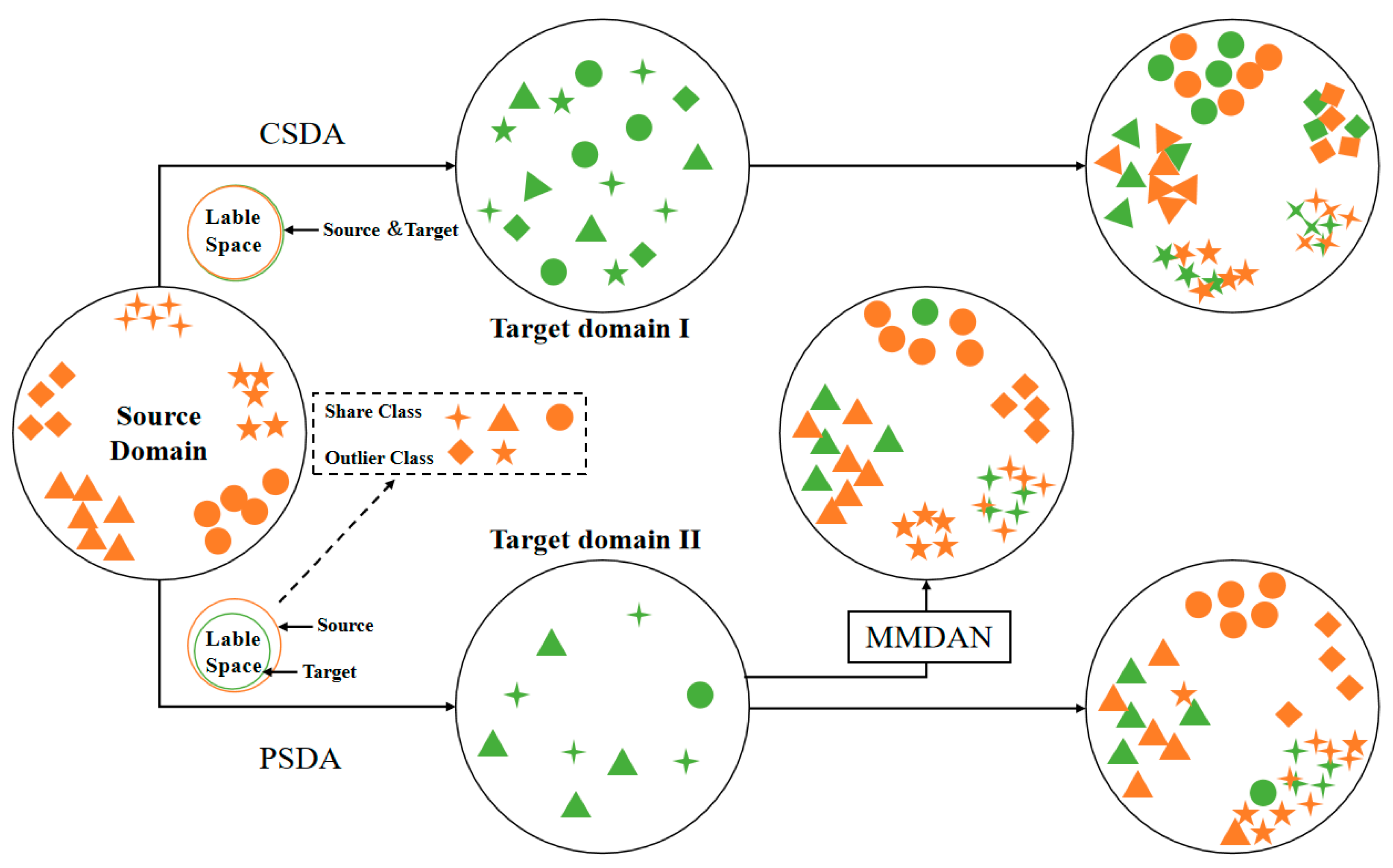
Transfer learning techniques have been extensively applied in industrial fault diagnosis and have achieved certain results. Nonetheless, prevailing methodologies often assume an identical label space for both the source and target domains, i.e., ${\mathrm{C}}_{\mathrm{t}}={\mathrm{C}}_{\mathrm{s}}$. In industrial applications, collecting a complete dataset is often a challenging task. As a result, a more realistic and challenging scenario arises where only a subset of classes from the target domain exist in the source domain, i.e., ${\mathrm{C}}_{\mathrm{t}}\subseteq {\mathrm{C}}_{\mathrm{s}}$. This particular scenario can be referred to as partial transfer fault diagnosis (PTFD). In the partial transfer learning problem, outlier data, which exist in the source domain but not in the target domain, will have a negative impact on the transfer process.

Research on partial transfer problems is emerging in intelligent fault diagnosis. In their study, Zhao et al. [25] introduced a weighted adversarial comparison approach for mitigating the impact of irrelevant source samples and reducing disparities in edge distributions in the context of partial domain fault diagnosis. Jiao et al. [26] presented a novel approach, known as the multi-weighted domain adversarial network (MWDAN), to address the challenges of PTFD. This approach encompasses the simultaneous incorporation of class-level and instance-level weighting mechanisms, enabling the discrimination of the label space and providing a quantitative measure of data sample transferability. Zhao et al. [27] introduced a novel strategy called the multi-discriminator deep weighted adversarial network (MDWAN) approach. This approach incorporates a weight function that quantifies the contribution of source domain samples to both domain discriminators and classifiers.

Undoubtedly, several transfer methods highlighted above emphasize the utilization of weighting techniques to selectively transfer knowledge from the source domain. However, it is essential to acknowledge the potential risks associated with relying solely on classifiers or discriminators to exclude outliers. This precautionary approach is necessitated by the fact that variations in domain distributions, arising from alterations in operating conditions and environmental noise, may lead to erroneous estimations of the target label space. Therefore, it is imperative to consider these uncertainties when implementing knowledge transfer techniques.

In this paper, the authors propose a Multi-scale and Multi-view domain adversarial network specifically designed for scenarios involving partial domain adaptation learning, where the target domain has fewer categories than the source domain. To address the challenge of strong non-linear relationships in marine diesel engine data, the authors propose a deep separable convolutional (DSC) neural network model for feature extraction. This model effectively captures complex patterns and reduces computation by utilizing separable convolutions. To enhance domain adaptation, the authors introduce an auxiliary domain discriminator learning strategy. This strategy helps identify and filter outlier source samples, promoting the positive transfer of shared samples. By using the auxiliary domain discriminator, similarity weights between the source and target domains can be measured, facilitating effective knowledge transfer. Furthermore, the paper employs two classifiers with different viewpoints to predict the same sample. This approach aims to map the original data to a more suitable feature space, ultimately improving the quality and discrimination ability of the extracted features. In summary, the proposed Multi-scale and Multi-view domain adversarial network combines the use of deep separable convolutional neural networks, auxiliary domain discriminator learning, and multiple classifiers to tackle the challenges of partial domain adaptation learning. This approach enhances the efficiency and effectiveness of knowledge transfer and feature extraction in such scenarios.

This paper introduces several key ideas and contributions:

• The introduction of a novel network called MMDAN to address the partial set domain adaptation problem in marine diesel engine fault diagnosis. MMDAN overcomes the limitation of having an identical label space between the source and target domains.
• A DSC-based multi-scale feature extraction method is proposed as part of MMDAN. The method replaces traditional convolutional layers with DSC layers, which not only extract useful information effectively but also reduce the number of parameters and computational effort. The inclusion of a residual connection layer further enhances the extraction accuracy.
• The paper presents a multi-scale classifier strategy where the same sample is predicted using two classifiers with different viewpoints. These classifiers have different weights and predict the same sample from distinct perspectives. Agreement between the predictions of the two classifiers confirms the applicability of the features extracted by the shared feature extractor.
• The proposed auxiliary discriminator learning strategy involves the use of an additional discriminator to quantify the transferability of source domain samples. This auxiliary discriminator helps identify and filter outlier samples, reducing distribution differences between the source and target domains. The partial set domain adaptation (PSDA) approach, incorporating the auxiliary discriminator, demonstrates improved diagnostic performance, even when test data are contaminated with noise.

These contributions collectively enhance the effectiveness and robustness of fault diagnosis in marine diesel engines, particularly in scenarios involving partial set domain adaptation and noisy test data. As for the remaining parts of the paper, they are arranged as follows: Section 2 gives an overview of transfer learning theory. This section covers fundamental concepts and methodologies related to transfer learning that form the basis for the proposed approach. Section 3 thoroughly presents the key components and steps of the proposed framework for fault detection and diagnosis. It describes the overall architecture and components of the MMDAN network, including the multi-scale feature extraction method, the multi-scale classifier strategy, and the auxiliary discriminator learning strategy. This section provides a comprehensive understanding of the proposed model’s design and functionality. Section 4 evaluates and compares the performance of the proposed model to other existing algorithms or approaches. This comparison is conducted using relevant datasets or experiments to highlight the superiority and effectiveness of the MMDAN network in addressing the PSDA problem in marine diesel engine fault diagnosis. Finally, Section 5 concludes the paper by summarizing the contributions and implications of the research.

2. Preliminaries

2.1. Problem Definition

According to [28,29,30], this paper defines domain, task, transfer learning, and domain adaptation as follows.

Domain contains two components, namely, the feature space X and the marginal probability distribution P(X), written as D = {X, P(X)}, where X = {x|x_i ∈ X, i = 1, ⋯, N} is the dataset containing N instances. In the context of industrial fault diagnosis scenarios, different domains can be defined based on variations in feature spaces or marginal probability distributions. These variations can arise due to different working conditions, locations, or specific machines being considered. It should be emphasized that the marginal distribution P(X) is usually an implicit function, i.e., it is difficult to obtain an explicit expression for this function, and usually, the domain is instantiated as $D={\left\{x_i,y_i\right\}}_{i=1}^n$.

Task: when given a particular domain D, the task T contains two parts, namely, the label space Y and a prediction function f (·), denoted as T = {Y, f (·)}, where Y = {y|y_i ∈ Y, i = 1, ⋯, N} is the set of labels of the corresponding instances in D, and the prediction function f (·) is obtained in the learning process of the algorithm on the samples. The mapping function f (·) can also be defined as f (x) = P (y|x), denoted as a nonlinear implicit function that can connect the relationship between the input instances and the prediction decisions, expected to be learned from the given dataset. Different tasks are defined as different label spaces, so different categories and types of faults can be treated as different tasks.

Domain Adaptation: DA in transfer learning deals with the challenge of different data distributions between the source and target domains. Its objective is to transfer knowledge from the source domain in order to enhance the learning performance in the target domain by minimizing the distribution discrepancy.

In this paper, we study the PSDA approach in fault diagnosis; let $D_s={\left\{\left(x_i^s,y_i^s\right)\right\}}_{i=1}^{n_s}$ and $D_t={\left\{\left(x_i^t\right)\right\}}_{i=1}^{n_t}$ denote the source domain with n_s labeled samples and the target domain with n_t unlabeled samples, respectively. Assuming that the source label space contains the target label space, i.e., ${\mathrm{C}}_{\mathrm{t}}\subseteq {\mathrm{C}}_{\mathrm{s}}$, the source and target data are collected from different probability distributions due to the change in operating conditions, i.e., P(X^s) ≠ P(X^t), as shown in Figure 1.

2.2. DA Adversarial Training Method

In 2014, Goodfellow introduced the concept of Generative Adversarial Networks (GANs) [31], which are designed as a generative framework to align with the data distribution of the training set. A typical GAN comprises two key components: a generator that learns the inherent distribution within the training data, and a discriminator/critic that discerns between samples from the original training set. When training the GAN, we usually use a max–min alternating optimization strategy. On one hand, the objective is to minimize the loss of the feature extractor, enabling it to produce more realistic samples. On the other hand, the aim is to maximize the loss of the discriminator, preventing it from accurately discerning whether a given sample originates from the real dataset or the generated dataset.

Inspired by GANs, Ganin et al. [32,33] pioneered the integration of an adversarial mechanism in neural network training, introducing their network as the Domain–Adversarial Neural Network (DANN). The domain–adversarial network consists of three components, a feature extractor G_f (parameter θ_f), classifier G_y (parameter θ_y), and domain discriminator G_d (parameter θ_d)—specifically, given the input x and its predicted label y, G_f is used to receive data from the source or target domain for feature extraction; G_y is used to receive the extracted features for task classification (it can also be used for other types of downstream tasks); G_d is utilized to determine whether the input features originate from the source domain or the target domain. The objective function formula is shown below.

$$E\left({\theta }_f,{\theta }_y,{\theta }_d\right)=\frac{1}{n_s}{\displaystyle \sum }_{x_i\in D_s}{L}_y\left(G_y\left(G_f\left(x_i\right)\right),y_i\right)-\frac{\theta }{n_s+n_t}{\displaystyle \sum }_{x_i\in D_s{{\displaystyle \cup }}^{\text{}}{D}_t}{L}_d\left(G_d\left(G_f\left(x_i\right)\right),d_i\right)$$

(1)

where L_y and L_d are the cross-entropy losses of G_y and G_d, respectively, n_s and n_t are the sample numbers of the source and target, respectively, and d_i is the domain label. θ is the tradeoff coefficient.

First, the domain adversarial network optimizes the parameters θ_f and θ_y of the feature extractor G_f and classifier G_y. This is achieved by minimizing the classification loss in relation to the loss of the feature extractor.

$$\left({\widehat{\theta }}_f,{\widehat{\theta }}_y\right)=\arg \underset{{\theta }_f,{\theta }_y}{\min }E\left({\theta }_f,{\theta }_y,{\widehat{\theta }}_d\right)$$

(2)

Then, its parameter θ_d is optimized by maximizing the loss of the domain discriminator G_d.

$${\widehat{\theta }}_d=\underset{ {\theta }_d}{\arg max}E\left({\widehat{\theta }}_f,{\widehat{\theta }}_s,{\theta }_d\right)$$

(3)

where ${\widehat{\theta }}_f,{\widehat{\theta }}_s$, and ${\widehat{\theta }}_d$ represent the optimal value of the saddle point, and the domain adversarial network can be used for the scenario where the same label is shared between the source and target domains, i.e., C_s = C_t, which is optimized by introducing a gradient reversal layer (GRL) using a gradient descent optimizer (e.g., SGD, Adam, or RMSProp) during the backpropagation process.

3. Proposed Method

In the PSDA problem, the source category is asymmetric to the target category. As a result, the source label space can be naturally divided into two subsets: the shared space (which is identical to the target label space) and the outlier space (which differs from the target label space).

In this paper, a Multi-scale and Multi-view domain adversarial network-based industrial process partial set fault detection algorithm is proposed, and the network structure is shown in Figure 2. Specifically, MMDAN consists of Multi-scale Feature Extractor G, Multi-view Classifier C, Auxiliary Domain Discriminator D₁, and Domain Discriminator D₂, and the parameters are shown in Figure 3.

3.1. Feature Extractor Structure G

The feature extractor G employs a multi-scale feature extraction module, consisting of two DSC layers with distinct weights, to extract multi-view features from two domains. This approach replaces conventional convolutions with DSCs, which have a smaller parameter count. Consequently, the model complexity is effectively reduced, leading to shorter training times. Furthermore, the integration of DSC blocks with different parameters enables the multi-scale feature extraction strategy. This strategy facilitates the extraction of multi-scale features that encompass a richer set of diagnostic information, along with complementary insights, by combining the outputs of these DSC blocks.

As illustrated in Figure 4, there is a data segment comprising K channels, the width and height of the convolution kernel are D_m and D_n, respectively, and the parameters of this part are D_m × D_n × K; then, after point-by-point convolution, the size of the convolution kernel is 1 × 1 × K. If we want N feature maps, then the parameters of point-by-point convolution are K × 1 × 1 × N. The parameters of DSC P_DSC are D_m × D_n × K + K × 1 × 1 × N. The parameters of ordinary convolution are D_m × D_n × K × N. The optimization equation for both is shown in the following equation (the computation of the multiplication method is ignored since it is much larger than that of the addition method):

$$\frac{P_{DSC}}{P_{CNN}}=\frac{D_m\times D_n\times K+K\times 1\times 1\times N}{D_m\times D_n\times K\times N}=\frac{1}{K}+\frac{1}{D_m\times D_n}$$

(4)

As demonstrated by Equation (1), the computational efficiency of DSC exceeds that of traditional CNNs. This is primarily due to the reduction in the number of parameters computed, while still maintaining satisfactory prediction accuracy. Thus, the key advantage of DSC, as an optimized variant of CNN, lies in its superior computational efficiency and its ability to effectively reduce the parameter count within adversarial networks.

Meanwhile, in order to effectively suppress the overfitting phenomenon, the maximum pooling layer and the average pooling layer are used to reduce the feature dimension, the attention layer helps to eliminate redundant information, and the residual connection is designed to prevent gradient degradation and information loss during the training process and facilitate feature extraction at different levels. The feature f can be represented as

$$f=\mathsf{\sigma }\left[{\left(w_f\right)}^{T}x+b_f\right]$$

(5)

where $w_f$ indicates the weight matrix and $b_f$ is the bias vector, and x is the input vector of the last pooling layer.

3.2. Auxiliary Domain Discriminator D

In the context of the PSDA, the coexistence of distinct label spaces in the source and target domains, denoted as Ct ⊆ Cs, presents a challenge for direct adversarial training implementation. The presence of outlier classes in the source domain negatively impacts the test performance, as it implies that certain source outlier classes may not have corresponding classes in the target domain. Consequently, it becomes vital to disregard these outlier classes during the domain adaptation process. Nonetheless, this presents a challenge, since the target domain data lack supervision, making it difficult to determine the presence of faults within the target domain. To address this issue, a logical approach is to align known class samples between the two domains while disregarding the target outliers during domain adaptation. To achieve this, a similarity learning strategy is proposed. This strategy aims to quantify the contribution of each source class, aid the domain discriminator D₁ in estimating the similarity between target samples and source samples, and assign similarity weights to each target sample. Additionally, a secondary game is introduced between the domain discriminator D₂ and the feature generator G to explore the transferable features. Given that the label spaces of source outliers and target outliers are distinct, it is expected that the target data will exhibit significant dissimilarities compared to the outlier class data. Therefore, the probability of assigning the target data to the outlier class should be minimized. Accordingly, the error in domain label classification can serve as a reliable indicator of similarity. In this study, the similarity of the target sample is defined by Equation (6) for further analysis and evaluation.

$$\mathit{w}=L_{CE}\left(D_1\left(G\left(x^t\right)\right),d^t\right)$$

(6)

where $d^t$ denotes the ground-truth label of the target domain, and in addition, the min–max normalization method is used to show the relative similarity of different target samples.

$$w_j=\frac{w_j-\max \left(\mathit{w}\right)}{\max \left(\mathit{w}\right)-\min \left(\mathit{w}\right)+\epsilon }$$

(7)

where $w_j$ represents the similarity weight assigned to the j-th target sample, and ε denotes a small positive value. This formulation ensures that the similarity weights assigned to the shared classes surpass those assigned to the outlier classes. Given the limited contribution of outlier class samples, domain adaptation can be selectively executed solely on the shared classes between the domains, thereby avoiding any detrimental negative transfer and promoting positive transfer. It should be noted that the auxiliary domain discriminator D₁ does not partake in adversarial training alongside the feature generator. Consequently, the loss function, denoted as $L_{D_1}$, exclusively updates the parameters ${\mathit{\theta }}_{D_1}$.

$$L_{D_1}\left({\mathit{\theta }}_G,{\mathit{\theta }}_{D_1}\right)=\frac{1}{n_s}{\displaystyle \sum }_{i=1}^{n_s}{L}_{CE}\left(D_1\left(G\left(x_i^s\right),d_i^s\right)\right)+\frac{1}{n_t}{\displaystyle \sum }_{j=1}^{n_t}{L}_{CE}\left(D_1\left(G\left(x_j^t\right),d_j^t\right)\right)$$

(8)

Let $d_i^s$ and $d_j^t$ represent the defined domain labels of the i-th source sample and the j-th target sample, respectively. In adversarial learning, the target samples undergo min–max normalization, and similarity weights are then assigned to them in order to minimize the disparity in domain distributions. As such, the objective of weighted adversarial learning can be formally defined as follows:

$$L_{D_{\mathrm{adv}}}^W\left({\mathit{\theta }}_G,{\mathit{\theta }}_{D_1},{\mathit{\theta }}_{D_2}\right)=\frac{1}{n_s}{\displaystyle \sum }_{i=1}^{n_s}{L}_{CE}\left(D_2\left(G\left(x_i^s\right),d_i^s\right)\right)+\frac{1}{n_t}{\displaystyle \sum }_{j=1}^{n_t}{w}_j{L}_{CE}\left(D_2\left(G\left(x_j^t\right),d_j^t\right)\right)$$

(9)

D₁ distinguishes the importance of different failure classes and extracts quality domain-invariant representations specifically for the shared classes. In the case of samples originating from outlier source classes, their respective loss functions are assigned relatively smaller weights, thereby minimizing their impact during training. On the other hand, for samples originating from cross-domain shared classes, a higher weight is assigned to the target loss function. The intention behind this is to mitigate domain bias and facilitate a better alignment between the source and target domains for the shared labeled samples. By doing so, a more effective matching between the two domains is achieved. The domain discriminator D₂ plays a minimax game with the feature generator G to explore transferable features.

3.3. Multi-View Classifiers C

Within this section, a novel multi-view predictive adversarial network is presented, encompassing two modules with distinct views within the classifier component. While the samples from the source domain possess sufficient labels, those from the target domain lack such annotations. Consequently, the enhancement of accuracy for unlabeled target domain samples through gradient descent becomes unfeasible. In order to bolster accuracy within the target domain, two classifiers are devised, each adopting a unique perspective on a given sample. The weights of these classifiers are constrained to guarantee their divergent viewpoints. Specifically, y¹ and y² denote the categories with the highest probability of prediction. It is posited that samples lacking labels can be accurately predicted when both classifiers concur on the prediction, i.e., y¹ = y².

In the case of the source domain, where a substantial number of labels are available, the network can be trained using traditional supervised learning methods. The commonly employed metric for such training is the cross-entropy loss, which can be expressed as follows:

$$L_Y=\frac{1}{n_s}{\displaystyle \sum }_{i=1}^{n_s}\left[L_y\left(G_y^1\left(G_f\left(x_i;{\theta }_f\right);{\theta }_y\right),y_i\right)+L_y\left(G_y^2\left(G_f\left(x_i;{\theta }_f\right);{\theta }_y\right),y_i\right)\right]$$

(10)

where $L_y$ is the consistent prediction loss, and $n_s$ denotes the number of source domain data. $G_y^1$ and $G_y^2$ denote two different classifiers.

Under the guidance of source domain supervision, the shared feature extractor and the two distinct classifiers are updated iteratively until achieving accurate classification. This is accomplished through the alignment of multi-view predictions and auxiliary domain adversarial training.

To enhance the generalization capability of the shared feature extractor and the two classifiers within the target domain, Mean Squared Error (MSE) loss is typically employed as an indicator of prediction consistency. Mathematically, MSE loss can be expressed as follows:

$$L_{Con}=\frac{1}{n}{\displaystyle \sum }_i^n\Vert G_y^1\left(G_f\left(x_f;{\theta }_f\right);{\theta }_y\right)-G_y^2\left(G_f\left(x_f;{\theta }_f\right);{\theta }_y\right)\Vert$$

(11)

where n is the number of source domain data, and $G_y^1\left(G_f\left(x_f;{\theta }_f\right);{\theta }_y\right)$ and $G_y^2\left(G_f\left(x_f;{\theta }_f\right);{\theta }_y\right)$ denote the predictions of two different classifiers.

To ensure the accurate prediction of target samples, we aim for classifiers C₁ and C₂ to classify samples based on different viewpoints. Therefore, we impose a constraint on the weights of C₁ and C₂ to be distinct, allowing the two classifiers to predict the same sample in the shared feature space from different perspectives. In the cost function, we include the term $\left|W_1{}^T{W}_2\right|$, where W₁ and W₂ represent the weights of the fully connected layers in C₁ and C₂, respectively. Mathematically, this loss for Multi-View constraints can be expressed as follows:

$$L_W=\left|W_1{}^T{W}_2\right|$$

(12)

3.4. The Overall Function Optimizes the Object

In summary, the overall objectives of the proposed method are:

$$E\left({\theta }_f,{\theta }_D,{\theta }_y\right)=\alpha L_{D_{\mathrm{adv}}}^W+\beta L_Y+\gamma L_{Con}+\delta L_W$$

(13)

The network parameters are trained to achieve:

$$\left({\widehat{\theta }}_f,{\widehat{\theta }}_{y_1},{\widehat{\theta }}_{y_2}\right)=\arg \underset{{\theta }_f,{\theta }_{y_1},{\theta }_{y_2}}{\min }E\left({\theta }_f,{\theta }_{y_1},{\theta }_{y_2},{\widehat{\theta }}_{d_2}\right)$$

(14)

$${\widehat{\theta }}_{d_2}=\arg \underset{{\theta }_{d_2}}{\max E}\left({\widehat{\theta }}_f,{\widehat{\theta }}_{y_1},{\widehat{\theta }}_{y_2},{\theta }_{d_2}\right)$$

(15)

$${\widehat{\theta }}_{d_1}=\arg \underset{{\theta }_{d_1}}{\max }{E}_{d_1}$$

(16)

where α, β, γ, and δ respectively are the coefficients of $L_{D\_\mathrm{adv}}^W, L_Y, L_{Con},$ and $L_W$. The optimization process utilizes the Stochastic Gradient Descent (SGD) algorithm and incorporates a GRL during the backpropagation process.

The complete diagnostic procedure of the proposed MMDAN can be summarized as follows.

Step 1: Before using the samples from the source and target domains as inputs to the network, the data undergo preprocessing, which typically includes normalization to ensure the data are within a specific range. This normalization step helps to standardize the input data and ensure that they have similar scales or distributions. Additionally, the samples from the source and target domains are divided into separate sets for training and testing. This division is crucial for evaluating the performance of the MMDAN model accurately and avoiding overfitting.

Step 2: During this step, the MMDAN model performs feature extraction using Equation (5), incorporates an auxiliary discriminator D₁ to highlight the importance of source domain samples, calculates the losses of both D₁ and D₂ using Equations (8) and (9), respectively, and employs multiple classifiers with different views to predict the classes based on the shared features extracted by G_f.

Step 3: The optimization objective, as defined by Equation (13), combines the various loss terms and incorporates Equation (12) to promote the incorporation of different views from the two classifiers during the training process. This optimization objective guides the learning process of the MMDAN model towards achieving better performance and adaptation in the target domain.

Step 4: After the model training is complete, the samples from the target domain test set are fed into the shared feature extractor, and the average of the predictions from the two classifiers is taken to generate the final prediction result for these samples.

4. Experimental Research

4.1. Dataset Description

To evaluate the effectiveness of the approach on the PTFD problem, a series of fault diagnosis experiments were conducted using data from seven 57,000 dwt bulk carriers from STX (D-2001, D-2002, D-2003, D-2004, D-2005, D-2009, D-2010). These vessels were equipped with a TCA66-20041 turbocharger and featured the 6S50MC-C7 main engine model. Detailed specifications of the diesel engine and turbocharger parameters can be found in

Table 1. Main specifications of the 6S50MC diesel engine.

Parameters	Value
Cylinder numbers	6
Number of strokes	2
Rated speed (r/min)	127
Continuous output (kW)	9480
Mean effective pressure (bar)	1.9
Bore (mm)	500
Stroke (mm)	2000
Stroke/bore	4
Brake Specific Fuel Consumption (g/kWh)	178.35

and

Table 2. Main specifications of the TCA66 turbocharger.

Parameters	Value
Exhaust turbine type	Axial Flow
Compressor type	Centrifugation style
Compressor pressure ratio	3.75
Compressor flow rate (kg/s)	24
Nominal speed (rpm)	14,250
Maximum allowable temperature (/°C)	500
Maximum allowable speed (rpm)	16,000
Turbine pressure ratio	3.24
Weight (kg)	5500

, respectively. Simulating failures on actual ships to obtain fault samples can not only result in significant economic losses but also pose a threat to maritime safety. For diesel engines of the same model, despite being sourced from different vessels, their performance parameter variations follow a similar pattern due to their identical principles, with minimal differences. Therefore, this study collects samples from the engine simulators.

The test data consist of the normal data of the host system, six types of performance fault data (Turbocharger filter screen dirty blocked, Dirty blockage of air inlet, Dirty blockage of exhaust port, Air cooler smudge, Turbine nozzle carbon deposits, and Air plug of cylinder liner cooling water cavity), and four types of abnormal boundary condition data (Insufficient cooling of cylinder liner, Insufficient cooling of piston, Air cooler cooling water inlet temperature too high, and Air cooler cooling water inlet temperature too low), and the dataset is classified as shown in

Table 3. Label information for the experimental dataset.

Data Type	Engine Conditions	Label
Health condition	Without any fault	1
Performance breakdown	Turbocharger filter screen dirty blocked	2
	Dirty blockage of air inlet	3
	Dirty blockage of exhaust port	4
	Air cooler smudge	5
	Turbine nozzle carbon deposits	6
	Air plug of cylinder liner cooling water cavity	7
Abnormal boundary condition	Insufficient cooling of cylinder liner	8
	Insufficient cooling of piston	9
	Air cooler cooling water inlet temperature too high	10
	Air cooler cooling water inlet temperature too low	11

.

4.2. Implementing Details and Comparing Methods

This study applies different strategies to partial transfer learning for comparison purposes. The parameters of all methods were determined based on the relevant literature and experimental requirements to achieve satisfactory performance. The network structure of MMDAN is shown in Figure 3. To ensure fairness in comparison, the proposed method, MMDAN, and the comparison method are all trained using the same learning rate, training batch size, and number of iterations. PyTorch is the software framework used to train the model, and Nvidia-2080Ti GPU is used to accelerate the computation. The final diagnostic results were performed by 10-replicate averaging experiments to reduce randomness and provide a comprehensive evaluation.

Specifically, the following methods are implemented:

(1)

Baseline: In the context of the paper, the baseline method refers to a simple network architecture consisting of a shared feature extractor and a classifier. The baseline method serves as a benchmark for assessing the extent of the performance improvements achieved through the proposed method’s incorporation of transfer learning mechanisms.

(2)

CIDA [34]: CIDA leverages classifier inconsistency as a means to minimize domain distribution differences. By comparing the predictions of the two classifiers, CIDA identifies discrepancies or inconsistencies in their outputs. These inconsistencies serve as indicators of domain-specific information and can be used to guide the adaptation process.

(3)

IWAN [35]: IWAN is a partial transfer learning method specifically designed for computer vision tasks. It introduces an auxiliary domain discriminator to assess the importance or relevance of source domain samples during the adaptation process.

(4)

WANT [36]: WATN is a method specifically developed for local domain fault diagnosis. It employs adversarial training to learn both class discriminative features and domain invariant features and utilizes a weighted learning strategy to measure and control their contributions to the source classifier and domain discriminator.

(5)

MWDAN [26]: MWDAN is a network architecture that incorporates both an adaptive weighting mechanism and a domain adversarial network. This combination allows MWDAN to jointly design class-level and instance-level weighting mechanisms, which help to distinguish the label space and quantify the transferability of data samples during the domain adaptation process.

4.3. Experimental Analysis

4.3.1. Experimental Results

The experiment consists of 10 partial transfer learning tasks, denoted as T1–T10. These tasks aim to evaluate the effectiveness of the proposed partial transfer learning method. The experimental tasks and their details are presented in

Table 4. Experimental Task.

Transfer Task	Source Domain	Target Domain
M1	90%:1 2 3 4 5 6 7 8 9 10 11	75%:1 3 4 5 6 7 8 9 11
M2	90%:1 2 3 4 5 6 7 8 9 10 11	75%:1 2 5 6 7 8 10
M3	90%:1 2 3 4 5 6 7 8 9 10 11	75%:1 5 7 10
M4	90%:1 2 3 4 5 6 7 8 9 10 11	75%:1 3 9
M5	90%:1 2 3 4 5 6 7 8 9 10 11	75%:1
M6	90%:1 2 3 4 5 6 7 8 9 10 11	50%:1 2 3 5 6 7 9 10 11
M7	90%:1 2 3 4 5 6 7 8 9 10 11	50%:1 4 5 6 7 8 9
M8	90%:1 2 3 4 5 6 7 8 9 10 11	50%:1 2 6 8
M9	90%:1 2 3 4 5 6 7 8 9 10 11	50%:1 2 5
M10	90%:1 2 3 4 5 6 7 8 9 10 11	50%:1

. To simulate a real industrial scenario, the source domain includes data from all health conditions, while the target domain is designed to contain only a subset of the health conditions. It is important to note that the health condition categories for the target domain are selected randomly. In terms of data collection, 90% of the load on the host system is used to collect data for the source domain, while 75% and 50% of the load are used to collect data for the target domain. During training, both labeled samples from all health conditions in the source domain and unlabeled samples from partial health conditions in the target domain are utilized. The training set consists of 80% of the samples, while the remaining 20% are used for testing. The fault diagnosis results obtained from the experiments are presented in

Table 5. Classification accuracy of different methods on the dataset.

Task	Baseline	CIDA	IWAN	WATN	MWDAN	MMDAN
M1	47.39 ± 0.02	61.51 ± 1.22	73.59 ± 1.02	86.14 ± 4.14	88.04 ± 3.02	96.47 ± 1.25
M2	56.86 ± 0.05	66.27 ± 1.04	66.49 ± 0.35	80.37 ± 4.37	86.19 ± 2.19	95.51 ± 1.04
M3	41.53 ± 0.03	72.04 ± 1.35	75.06 ± 5.13	78.35 ± 4.56	84.47 ± 3.16	96.64 ± 1.28
M4	58.91 ± 0.04	75.63 ± 1.16	85.94 ± 9.73	72.98 ± 6.10	83.93 ± 3.73	95.32 ± 1.47
M5	54.57 ± 0.06	84.14 ± 1.53	91.46 ± 19.41	81.04 ± 6.46	88.59 ± 1.96	99.68 ± 0.24
M6	48.42 ± 0.06	60.33 ± 1.06	92.29 ± 0.46	83.37 ± 5.67	85.73 ± 3.79	96.47 ± 1.29
M7	55.15 ± 0.05	64.54 ± 1.26	75.70 ± 1.53	80.98 ± 5.25	79.86 ± 3.64	95.63 ± 1.19
M8	40.34 ± 0.04	70.37 ± 1.04	85.39 ± 0.59	79.62 ± 5.49	80.14 ± 3.41	95.41 ± 1.20
M9	55.98 ± 0.03	72.85 ± 0.24	92.70 ± 8.49	78.18 ± 13.47	77.49 ± 3.27	95.57 ± 1.10
M10	55.43 ± 0.06	82.49 ± 3.76	72.31 ± 25.96	84.23 ± 4.53	83.52 ± 2.47	99.09 ± 0.21
Average	51.46	71.02	81.09	80.53	83.80	96.58
Time(s)	832.7	1490.6	1876.5	1562.3	1286.4	1325.7

and Figure 5.

From Table 5 and Figure 5, several remarks are obtained.

(1)

In each transfer task, the proposed MMDAN has better diagnostic performance than the comparison method. The average accuracy of MMDAN is 96.58%, and in addition, it is worth noting that the proposed partial transfer learning method tends to exhibit a small standard deviation across different situations, reflecting the stability of MMDAN. In particular, for the challenging M4 and M9 transfer tasks, the accuracy of MMDAN remains as high as 95%.

(2)

Due to the CIDA multi-classifier mechanism, IWAN auxiliary domain discriminator mechanism, WATN weighted adversarial migration mechanism, and MWDAN class-level and instance-level weight mechanism, they outperform Baseline in most transmission tasks. However, their average accuracy is still 45.12%, 25.56%, 15.49%, and 12.78% lower than MMDAN, respectively.

(3)

Table 5 also provides insights into the average computation times of the different methods. Notably, the proposed method demonstrates relatively fast computation times, typically completing within 10 min in relevant cases. Compared to the other methods, the computation time of the MMDAN method is slightly longer. However, this difference is considered small and acceptable, especially considering that partial transfer fault diagnosis is commonly performed offline. As a result, the computational burden introduced by MMDAN remains within reasonable limits. The experimental findings indicate a favorable trade-off between accuracy and speed with the MMDAN method. While it achieves good performance accuracy-wise, it also manages to keep computation times at an acceptable level. This balance between accuracy and speed enhances the practical applicability and efficiency of the proposed MMDAN method in real-world settings.

A confusion matrix is used to provide a detailed analysis of the accuracy of the method. In this case, the diagnostic results of both MWDAN and the proposed method for task M6 are presented in Figure 6. In particular, there is a significant improvement of 22% for fault type 5 and of 20% for fault type 6 when comparing the proposed method to MWDAN. This improvement highlights the effectiveness of the proposed method in accurately detecting and diagnosing these specific fault types.

In order to reflect the advantages of the MMDAN method, M3, M4, and M7 are selected to calculate the F-score and AUC. The results are shown in

Table 6. Statistical results of the dataset.

Methods	M3		M4		M7
	F-Score	AUC	F-Score	AUC	F-Score	AUC
Baseline	0.8427	0.9645	0.7526	0.9531	0.7351	0.9295
CIDA	0.6364	0.9026	0.5014	0.8753	0.9148	0.9065
IWAN	0.6919	0.9241	0.8642	0.9254	0.6775	0.9292
WATN	0.8225	0.9593	0.8098	0.9327	0.8546	0.9387
MWDAN	0.8568	0.9647	0.8360	0.9654	0.8237	0.9526
MMDAN	0.9687	0.9952	0.9546	0.9850	0.9622	0.9924

. Based on the outcomes obtained from the selected cases, it can be concluded that the MMDAN method proposed in this study achieves the highest F-score and AUC metrics.

4.3.2. Ablation Experiment

To further test the effectiveness of the MMDAN method, ablation experiments are designed to investigate the effect of noisy data on the classification performance and to explore the effect of a multi-scale feature extraction structure and multi-view classifier on the detection accuracy and speed. Two ablation research schemes are designed based on the MMDAN method, namely, NoDSC and NoMC. The two network structures are generally the same as MMDAN, with the difference being that, in NoDSC, the DSC structure of the original MMDAN is changed into a CNN structure, and in NoMC, the multi-view classifier in the original MMDAN is changed into a single-view classifier composition. All models are trained using the original data and evaluated on the noisy data.

Table 7. Classification accuracy of different methods on noise data.

Task	Baseline	CIDA	IWAN	WATN	MWDAN	NoDSC	NoMC	MMDAN
M6	65.35	73.55	69.14	72.50	76.24	89.61	72.62	92.58
M7	60.24	67.28	58.65	68.13	75.12	88.29	70.87	90.47
M9	51.27	61.49	50.34	61.49	65.36	86.80	65.40	88.43
Average	58.95	67.44	59.37	67.37	72.24	88.23	69.63	90.49
Time	858.4	1452.1	1905.7	1512.4	1239.3	2034.6	1314.9	1289.8

presents the findings of the proposed method and other comparative methods.

As observed in Table 7, the diagnostic accuracy of all the methods has decreased. This can be attributed to the fact that the test data, which include auxiliary noise, further obscure valuable information, resulting in a greater variation in the data distribution across domains. As can be seen from Table 7, compared with MMDAN, the accuracy of NoDSC does not change significantly, but the average diagnosis time increases significantly by 57.7%, proving that the DSC structure can reduce the number of parameters and lower the operation cost. Compared with MMDAN, the average diagnosis time of the NoMC structure is slightly reduced, but the diagnosis accuracy is greatly reduced by 20.86%, proving that the classifier of two different views has a positive effect on partial transfer learning.

4.3.3. Feature Visualization Analysis

In order to visualize the effectiveness of the MMDAN method, the t-distribution stochastic neighbor embedding (t-SNE) technique is employed to visualize the feature distribution of the various methods. In this work, the complexity is set to a constant value of 100. Figure 7 and Figure 8 depict the high-dimensional feature space represented as a two-dimensional feature distribution. In these visualizations, circles represent classes in the source domain, while triangles represent classes in the target domain. The different colors within the same shape indicate distinct running conditions.

As can be seen in Figure 7a and Figure 8a, for the original samples, the feature representations between all health conditions overlap severely, resulting in incorrect classification in both the source and target domains. Figure 7b and Figure 8b show the visualized feature distribution of MMDAN under the M4 and M8 tasks, and it can be seen that the MMDAN method reduces the overlap between distinct classes and the difference in feature distribution between the source and target domains. For example, S1 and others display well-defined classification boundaries, facilitating accurate class prediction by the classifier. Moreover, there is a certain degree of clustering between the source domain S1 and the target domain T1, which helps bridge the gap between the two domains. This indicates that MMDAN is capable of learning more category-distinct but domain-invariant features. The visualization results demonstrate that MMDAN has a stronger capability of partial transfer fault diagnosis.

4.3.4. Experimental Conclusion

To verify the effectiveness of the proposed model in this paper, it is compared with Baseline, CIDA, IWAN, WANT, and MWDAN. First, the time required for the fault diagnosis of different methods is compared, and the results show that there is not much difference between these methods in terms of diagnosis time, but the average accuracy of MMDAN is 96.58%, which is 45.12%, 25.56%, 15.49%, and 12.78% better than that of the above methods, respectively, Overall, the experimental results support the claim that MMDAN effectively reduces the distribution differences between domains and surpasses existing methods in the context of partial transfer learning. This highlights the potential of MMDAN as a promising approach for addressing domain shifts and improving knowledge transfer in partial transfer learning scenarios. There may be several reasons for the exceptional performance of MMDAN. First, using the DSC layer can effectively reduce the input dimension of the model. By processing features at different scales, the DSC layer captures information at both local and global levels, allowing for a more comprehensive understanding of the input data. This reduction in dimensionality helps to avoid the curse of dimensionality and improve the efficiency of the model. By integrating the approach of building a multi-view classifier with auxiliary domain adversarial training, several benefits can be achieved. First, the strategy enables the adaptive identification and filtration of irrelevant source samples. This means that only the most relevant and informative source samples are utilized, thereby improving the quality and efficiency of the knowledge transfer process. Second, the combination of multi-view classifier construction and auxiliary domain adversarial training aids in minimizing the distribution differences among domains in the shared label space. This is crucial for effective knowledge transfer, as reducing the domain discrepancy enhances the transferability of learned knowledge from the multi-labeled source domain to the unlabeled target domain.

5. Conclusions

An MMDAN method is proposed for partial transfer fault diagnosis. This method uses the DSC layer to form a multi-scale feature extractor, and by constructing a strategy combining multi-view classifier and auxiliary domain adversarial training, it can adaptively identify and filter irrelevant source samples and minimize the distribution difference across domains in the shared label space so as to effectively realize the transfer of knowledge from the multi-label source domain to the target domain without labels. In addition, we performed an ablation analysis to verify the importance of the highlighted modules and establish their contribution to the suggested framework. The framework is evaluated on a marine diesel engine dataset to show its advantages. Comparative experiments show that the method is effective in reducing the distribution differences between different domains and outperforms existing partial transfer learning methods. In conclusion, the fault diagnosis method presented in this paper offers valuable insights for the health management of marine diesel engine systems. The findings and techniques developed can serve as a reference for ensuring the reliable operation and maintenance of these systems. Looking ahead, future work will concentrate on the online fault diagnosis of marine diesel engine systems, which is more applicable and practical in real shipping scenarios. By developing methods that enable real-time fault detection and diagnosis, the aim is to improve the efficiency and effectiveness of maintenance activities, minimize downtime, and enhance the overall performance of marine diesel engine systems.

References

1. Tan, Y.; Zhang, J.; Tian, H.; Jiang, D.; Guo, L.; Wang, G.; Lin, Y. Multi-Label Classification for Simultaneous Fault Diagnosis of Marine Machinery: A Comparative Study. Ocean. Eng. 2021, 239, 109723. [Google Scholar] [CrossRef]
2. Lazakis, I.; Raptodimos, Y.; Varelas, T. Predicting Ship Machinery System Condition through Analytical Reliability Tools and Artificial Neural Networks. Ocean. Eng. 2018, 152, 404–415. [Google Scholar] [CrossRef] [Green Version]
3. Zeng, H.; Zhao, Y.; Wang, T.; Zhang, J. Defense Strategy against False Data Injection Attacks in Ship DC Microgrids. J. Mar. Sci. Eng. 2022, 10, 1930. [Google Scholar] [CrossRef]
4. Qi, J.; Zhang, J.; Meng, Q. Auxiliary Equipment Detection in Marine Engine Rooms Based on Deep Learning Model. J. Mar. Sci. Eng. 2021, 9, 1006. [Google Scholar] [CrossRef]
5. Wang, R.; Chen, H.; Guan, C. Random Convolutional Neural Network Structure: An Intelligent Health Monitoring Scheme for Diesel Engines. Measurement 2021, 171, 108786. [Google Scholar] [CrossRef]
6. Han, P.; Li, G.; Skulstad, R.; Skjong, S.; Zhang, H. A Deep Learning Approach to Detect and Isolate Thruster Failures for Dynamically Positioned Vessels Using Motion Data. IEEE Trans. Instrum. Meas. 2021, 70, 1–11. [Google Scholar] [CrossRef]
7. Kim, J.; Lee, T.; Lee, S.; Lee, J.; Lee, W.; Kim, Y.; Park, J. A Study on Deep Learning-Based Fault Diagnosis and Classification for Marine Engine System Auxiliary Equipment. Processes 2022, 10, 1345. [Google Scholar] [CrossRef]
8. Ftoutou, E.; Chouchane, M. Diesel Engine Injection Faults’ Detection and Classification Utilizing Unsupervised Fuzzy Clustering Techniques. Proc. Inst. Mech. Eng. Part C J. Mech. Eng. Sci. 2019, 233, 5622–5636. [Google Scholar] [CrossRef]
9. Diez-Olivan, A.; Pagan, J.A.; Sanz, R.; Sierra, B. Data-Driven Prognostics Using a Combination of Constrained K-Means Clustering, Fuzzy Modeling and LOF-Based Score. Neurocomputing 2017, 241, 97–107. [Google Scholar] [CrossRef] [Green Version]
10. Cheng, C.; Zhou, B.; Ma, G.; Wu, D.; Yuan, Y. Wasserstein Distance Based Deep Adversarial Transfer Learning for Intelligent Fault Diagnosis with Unlabeled or Insufficient Labeled Data. Neurocomputing 2020, 409, 35–45. [Google Scholar] [CrossRef]
11. Li, F.; Chen, J.; Pan, J.; Pan, T. Cross-Domain Learning in Rotating Machinery Fault Diagnosis under Various Operating Conditions Based on Parameter Transfer. Meas. Sci. Technol. 2020, 31, 085104. [Google Scholar] [CrossRef]
12. Han, T.; Liu, C.; Wu, R.; Jiang, D. Deep Transfer Learning with Limited Data for Machinery Fault Diagnosis. Appl. Soft Comput. 2021, 103, 107150. [Google Scholar] [CrossRef]
13. Lee, J.; Kim, M.; Ko, J.U.; Jung, J.H.; Sun, K.H.; Youn, B.D. Asymmetric Inter-Intra Domain Alignments (AIIDA) Method for Intelligent Fault Diagnosis of Rotating Machinery. Reliab. Eng. Syst. Saf. 2022, 218, 108186. [Google Scholar] [CrossRef]
14. Shao, J.; Huang, Z.; Zhu, J. Transfer Learning Method Based on Adversarial Domain Adaption for Bearing Fault Diagnosis. IEEE Access 2020, 8, 119421–119430. [Google Scholar] [CrossRef]
15. Jia, M.; Wang, J.; Zhang, Z.; Han, B.; Shi, Z.; Guo, L.; Zhao, W. A Novel Method for Diagnosing Bearing Transfer Faults Based on a Maximum Mean Discrepancies Guided Domain-Adversarial Mechanism. Meas. Sci. Technol. 2021, 33, 015109. [Google Scholar] [CrossRef]
16. Ruicong, Z.; Yu, B.; Zhongtian, L.; Qinle, W.; Yonggang, L. Unsupervised Adversarial Domain Adaptive for Fault Detection Based on Minimum Domain Spacing. Adv. Mech. Eng. 2022, 14, 16878132221088647. [Google Scholar] [CrossRef]
17. Shao, J.; Huang, Z.; Zhu, Y.; Zhu, J.; Fang, D. Rotating Machinery Fault Diagnosis by Deep Adversarial Transfer Learning Based on Subdomain Adaptation. Adv. Mech. Eng. 2021, 13, 168781402110402. [Google Scholar] [CrossRef]
18. Liu, X.; Cheng, W.; Zhang, L.; Chen, X.; Wang, S. An Intelligent Hybrid Bearing Fault Diagnosis Method Based on Transformer and Domain Adaptation. In Proceedings of the 2021 IEEE International Conference on Sensing, Diagnostics, Prognostics, and Control (SDPC), Weihai, China, 13–15 August 2021; pp. 304–310. [Google Scholar]
19. Wang, Y.; Ning, D.; Lu, J. A Novel Transfer Capsule Network Based on Domain-Adversarial Training for Fault Diagnosis. Neural. Process Lett. 2022, 54, 4171–4188. [Google Scholar] [CrossRef]
20. Wu, J.; Tang, T.; Chen, M.; Wang, K. The Application of a Lightweight Domain-Adversarial Neural Network in Bearing Fault Diagnosis. In Proceedings of the Advanced Manufacturing and Automation X, Zhanjiang, China, 12–13 October 2020; Wang, Y., Martinsen, K., Yu, T., Wang, K., Eds.; Springer: Singapore, 2021; pp. 312–320. [Google Scholar]
21. Di, Y.; Yang, R.; Huang, M. Fault Diagnosis of Rotating Machinery Based on Domain Adversarial Training of Neural Networks. In Proceedings of the 2021 IEEE 30th International Symposium on Industrial Electronics (ISIE), Kyoto, Japan, 20–23 June 2021; pp. 1–6. [Google Scholar]
22. Borgwardt, K.M.; Gretton, A.; Rasch, M.J.; Kriegel, H.-P.; Schölkopf, B.; Smola, A.J. Integrating Structured Biological Data by Kernel Maximum Mean Discrepancy. Bioinformatics 2006, 22, e49–e57. [Google Scholar] [CrossRef] [Green Version]
23. Liao, Y.; Huang, R.; Li, J.; Chen, Z.; Li, W. Deep Semisupervised Domain Generalization Network for Rotary Machinery Fault Diagnosis Under Variable Speed. IEEE Trans. Instrum. Meas. 2020, 69, 8064–8075. [Google Scholar] [CrossRef]
24. Sun, B.; Saenko, K. Deep CORAL: Correlation Alignment for Deep Domain Adaptation. In Proceedings of the Computer Vision—ECCV 2016 Workshops, Amsterdam, The Netherlands, 8–10 and 15–16 October 2016; Hua, G., Jégou, H., Eds.; Springer International Publishing: Cham, Switzerland, 2016; pp. 443–450. [Google Scholar]
25. Zhao, C.; Liu, G.; Shen, W. A Balanced and Weighted Alignment Network for Partial Transfer Fault Diagnosis. ISA Trans. 2022, 130, 449–462. [Google Scholar] [CrossRef]
26. Jiao, J.; Zhao, M.; Lin, J. Multi-Weight Domain Adversarial Network for Partial-Set Transfer Diagnosis. IEEE Trans. Ind. Electron. 2022, 69, 4275–4284. [Google Scholar] [CrossRef]
27. Wang, Z.; Cui, J.; Cai, W.; Li, Y. Partial Transfer Learning of Multidiscriminator Deep Weighted Adversarial Network in Cross-Machine Fault Diagnosis. IEEE Trans. Instrum. Meas. 2022, 71, 1–10. [Google Scholar] [CrossRef]
28. Pan, S.J.; Yang, Q. A Survey on Transfer Learning. IEEE Trans. Knowl. Data Eng. 2010, 22, 1345–1359. [Google Scholar] [CrossRef]
29. Tan, C.; Sun, F.; Kong, T.; Zhang, W.; Yang, C.; Liu, C. A Survey on Deep Transfer Learning. In Proceedings of the Artificial Neural Networks and Machine Learning—ICANN 2018, Rhodes, Greece, 4–7 October 2018; Kůrková, V., Manolopoulos, Y., Hammer, B., Iliadis, L., Maglogiannis, I., Eds.; Springer International Publishing: Cham, Switzerland, 2018; pp. 270–279. [Google Scholar]
30. Li, W.; Huang, R.; Li, J.; Liao, Y.; Chen, Z.; He, G.; Yan, R.; Gryllias, K. A Perspective Survey on Deep Transfer Learning for Fault Diagnosis in Industrial Scenarios: Theories, Applications and Challenges. Mech. Syst. Signal Process. 2022, 167, 108487. [Google Scholar] [CrossRef]
31. Goodfellow, I.; Pouget-Abadie, J.; Mirza, M.; Xu, B.; Warde-Farley, D.; Ozair, S.; Courville, A.; Bengio, Y. Generative Adversarial Nets. In Advances in Neural Information Processing Systems 27, Proceedings of the 28th Annual Conference on Neural Information Processing Systems 2014, Montreal, QC, Canada, 8–13 December 2014; Curran Associates, Inc.: Red Hook, NY, USA, 2014; Volume 27. [Google Scholar]
32. Ganin, Y.; Ustinova, E.; Ajakan, H.; Germain, P.; Larochelle, H.; Laviolette, F.; Marchand, M.; Lempitsky, V. Domain-Adversarial Training of Neural Networks. arXiv 2016, arXiv:1505.07818. [Google Scholar]
33. Ganin, Y.; Lempitsky, V. Unsupervised Domain Adaptation by Backpropagation. arXiv 2015, arXiv:1409.7495. [Google Scholar]
34. Jiao, J.; Zhao, M.; Lin, J.; Ding, C. Classifier Inconsistency-Based Domain Adaptation Network for Partial Transfer Intelligent Diagnosis. IEEE Trans. Ind. Inform. 2020, 16, 5965–5974. [Google Scholar] [CrossRef]
35. Zhang, J.; Ding, Z.; Li, W.; Ogunbona, P. Importance Weighted Adversarial Nets for Partial Domain Adaptation. In Proceedings of the 2018 IEEE/CVF Conference on Computer Vision and Pattern Recognition, Salt Lake City, UT, USA, 18–23 June 2018; pp. 8156–8164. [Google Scholar]
36. Li, W.; Chen, Z.; He, G. A Novel Weighted Adversarial Transfer Network for Partial Domain Fault Diagnosis of Machinery. IEEE Trans. Ind. Inform. 2021, 17, 1753–1762. [Google Scholar] [CrossRef]
Figure 1. Different scenarios of DA faults diagnosis.
Jmse 11 01527 g001
Figure 2. Framework of the proposed method.
Jmse 11 01527 g002
Figure 3. Network architecture of the proposed method.
Jmse 11 01527 g003
Figure 4. The structure diagram of DSC (a) Depthwise convolution, (b) Pointwise convolution.
Jmse 11 01527 g004
Figure 5. Experimental results of the dataset.
Jmse 11 01527 g005
Figure 6. Confusion matrices of testing accuracy on task M6 based on different methods.
Jmse 11 01527 g006
Figure 7. The distribution graph of the data in Task 4.
Jmse 11 01527 g007aJmse 11 01527 g007b
Figure 8. The distribution graph of the data in Task 8.
Jmse 11 01527 g008aJmse 11 01527 g008b