Abstract
We propose a robust nonlinear trajectory tracking design by integrating a nonlinear model transformation, robust disturbance eliminator, and trajectory generator for unmanned surface vessels influenced by modeling uncertainties and ocean environmental disturbances. We designed this nonlinear control law to help control unmanned surface vessels following any designated sail trajectory constructed by the trajectory generator. With cubic spline interpolation, this trajectory generator can generate arbitrary smooth trajectories. Simulation results show that the proposed nonlinear robust control law has precise trajectory tracking performance and a robustness property for unmanned surface vessels under harsh ocean environmental disturbances and modeling uncertainties.
1. Introduction
Unmanned surface vessels (USVs) have been developed since the end of World War II. Studies on USV control designs have grown rapidly for military, civil, and commercial purposes. They can execute tasks considered too hazardous or difficult for humans to undertake, such as mine sweep missions, subsea mining, monitoring, etc. In practice, well-developed USVs can sense harsh ocean environments and operate without human involvement. In the military, the Republic of Singapore Navy values the warfighting capabilities of USVs for maritime operations. The Republic of Singapore was the first country in Southeast Asia to deploy USVs since the early 2000s, such as the 9 m Rafael PROTECTOR USV [1], which is expected to significantly reduce human labor and prevent humans from undergoing dangerous missions. The Republic of Singapore Navy’s unmanned surface vessels also detected and neutralized underwater threats in January 2021. In commercial applications, the world’s first autonomous and zero-emission container vessel, “Yara Birkeland”, sailed on its maiden voyage from Oslo in November 2021 [2]. These applications prove that the growing demand for USVs will increase in future years. Well-developed USV control designs are important to ensure the safe operation of USVs on the ocean, which is full of external disturbances without a human captain onboard. An effective control law design guarantees that controlled USVs can track designated trajectories despite modeling uncertainties and environmental disturbances. To achieve this trajectory-tracking target, hundreds of works related to the control design of autonomous ships have been published over the past few decades. Many conventional controllers that do not consider USV dynamics, such as Fuzzy Logic, PI, or PID controllers, are proposed for ships [3,4,5,6]. Under certain operation conditions, these published controllers were useful for ships’ autonomous control designs. Unfortunately, control designs based on the existing literature are innately weak at modeling uncertainties and environmental disturbances. Therefore, they cannot deliver optimal control performance in practical USV applications. Two nonlinear control laws were developed for a simplified nonlinear ship model, referred to as the Norrbin nonlinear ship model [7,8]. By observing the dynamics of the Norrbin nonlinear ship model, it is apparent that it does not seem to fully consider USV dynamics (hull resistance, Coriolis and centripetal forces, etc.). From the control design perspective, the control output for compensating model approximation error of the controlled USV model will be high if the total model approximation error is significant. For these reasons, nonlinear control designs, such as a robust adaptive neural network control algorithm, nonlinear optimal control, or sliding mode control, have also been developed for USVs [9,10,11,12,13]. In [9,10,11], heading control designs of unmanned marine vehicles based on adaptive fuzzy or adaptive neural network control algorithms were investigated. These kinds of neural network control algorithms usually have high calculation costs and risk the inability to generate control commands in real-time to operate USVs. In [12], a recently published study featuring a closed-form control design for waypoint tracking problems in USVs proposed a complete nonlinear model. This nonlinear optimal control law has the simplest control structure because it is an analytical solution that performs satisfactory trajectory tracking performance without considering disturbance effects. However, environmental disturbances (waves, ocean currents, and wind) or modeling uncertainties are inevitable when USVs sail the ocean. Hence, the control performance of this less robust control design predictably degrades in an ocean environment. The authors of [13] delivered a modified sliding mode control law that used monitoring functions. In this paper, we describe the application of this control method in USVs and its promising trajectory-tracking results. To solve the aforementioned problems, we developed a nonlinear robust control law to quickly converge trajectory-tracking errors at a low calculation cost while considering USV dynamics and simultaneously eliminating modeling uncertainties and environmental disturbances. This proposed control law integrates a feedback linearization method, which cancels the nonlinear terms of trajectory-tracking error dynamics. It also includes a robust disturbance eliminator, which reduces the effects of modeling uncertainties and environmental disturbances. This paper is organized into the following sections: Section 2 provides a brief description of the dynamics of a controllable USV; Section 3 describes the proposed robust control law; Section 4 provides the simulation results and compares the proposed control method and its competitor to two scenarios; and Section 5 contains our conclusions.
2. Model of the Controlled USV
The six degrees of freedom (six DOF) USV motions can be described by their Body-frame and Earth frame, respectively. A Body frame with origin Ob is a coordinate frame designated for moving USVs. Ob is usually chosen as the point overlapping the center of gravity (CG). In Earth-frame, the motion of the earth has a minor effect on the USVs; hence, the Earth frame can be regarded as an inertial coordinate. The linear and angular velocities of a controlled USV can be described using the Body frame, and the position and orientation of the controlled USV can be obtained from the Earth frame, as shown in Figure 1 and Table 1.
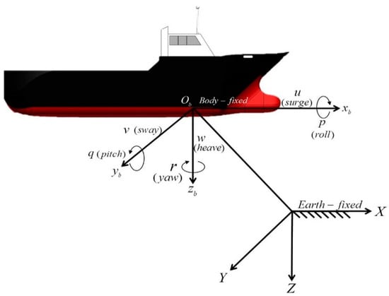
Figure 1.
Body and earth frames of USVs.

Table 1.
Coordinate notations of USVs in their body and earth frames.
Since USVs’ motions of heave, pitch, and roll are not controllable in practice, the six DOF model is remodeled as a three DOF dynamics equation in the Earth frame coordinate [14]:
where denotes the real-time position (X and Y) and heading angle (ψ) of USV in Earth frame coordinates and denotes the linear velocities with surge (u) and sway (v) in Body frame coordinates. In this investigation, represents the inertia mass; denotes the Coriolis and centripetal matrix; is the damping matrix; represents the control command; and represents the overall environmental disturbances induced by random waves (τwave), wind (τwind), and ocean currents (τcurrent) in Earth frame coordinates, respectively. Details of M, , D, and the transformation matrix are expressed as the following, respectively:
3. Nonlinear Control Design
We developed a trajectory generator and a robust nonlinear control design for USVs’ trajectory-tracking problem. In conventional tracking designs for USVs, the waypoint tracking method has been one of the main control designs. However, this kind of tracking design always results in a high-control gain output, and the outputs of actuators always exceed their physical limitations. For this reason, we propose a trajectory generator that constructs almost arbitrary smooth trajectories.
3.1. Trajectory Generator
Similar to the reasons described above, a smooth desired trajectory plays an important role in USVs’ control design because it ensures that controlled USVs can sail without changing directions and attitudes drastically, which is impossible and dangerous for installed actuators to perform. The cubic spline interpolation method [15] is often adopted to construct a smooth trajectory. Points (xd, yd) of the constructed continuous trajectory in this proposed cubic spline interpolation method are expressed by two piecewise third-order polynomials that pass through a set of desired waypoints , for g = 1,…, n, in Earth frame coordinates:
where ϖ is a path variable, and parameters ( and ) are unknown but designable coefficients.
Adopting the cubic spline interpolation method to generate a continuous 2-dimensional trajectory, each piecewise third-order polynomial must satisfy three conditions:
Condition 1:
The trajectory through the desired waypoints (xg, yg) and (xg+1, yg+1) must satisfy (8) and (9).
Condition 2:
The adopted third-order polynomial must be a continuous and smooth function that is at least twice differentiable.
Condition 3:
The path variable ϖ should be defined as (12) to prevent the slope of the trajectory from changing drastically.
Since two waypoints generate one path, there are 4(n − 1) unknown coefficients in (6) and (7) that must be identified:
where j = 1, 2, 3,…, n − 1.
This cubic spline interpolation method has unknown coefficients that can generate a continuous and smooth trajectory, as represented in matrix-vector form:
where,
and
where
The unknown coefficient vectors cx and cy in (13) and (14) can be obtained as follows:
The desired heading angle ψd is:
where,
3.2. Control Law Designs
For comparison purposes, we propose two nonlinear control laws: one that considers all disturbances (robust control design) and another (feedback linearization control design) that does not consider disturbance effects in its control law design.
3.2.1. Feedback Linearization Control Design (FL)
Referring to USV dynamics (1), if environmental disturbances and modeling uncertainties are omitted, dynamic equations of the controlled USV can be rewritten as:
Define the tracking error between the controlled USV and desired trajectory, which is generated by the proposed trajectory generator as:
where (Xd, Yd) is the desired position and ψd is the desired heading angle.
The first and second derivatives of (21) with respect to time yield are as follows:
By substituting (20) to (23), a trajectory-tracking error dynamic can be obtained describing the relationship between the desired trajectory and the controlled USV:
Select a nonlinear control law τη as follows:
where is
where control parameters λl > 0, for l = 1, …, 6.
Due to ψd ∈ C2, we have
By substituting the nonlinear control law of (25) with (24), a second-order trajectory-tracking error dynamic can be obtained:
where,
The trajectory-tracking error dynamics in (31) satisfy the Hurwitz condition, creating a set of control parameters λl where the roots of (31) are on the left-hand side of the s-plane. Based on this arrangement, the convergent property of the trajectory-tracking error e in (21) can be guaranteed as follows:
Achieving the convergent property of the trajectory-tracking error e(t) in (33) this control design does not consider environmental disturbances . Random environmental disturbances are inevitable, and eliminating modeling uncertainties is important to achieving a satisfactory trajectory-tracking performance. However, these two inherent characteristics impractically and unreasonably degrade the trajectory-tracking performance of the proposed FL control design and neglect the two inner and outer effects of USVs. Therefore, we investigated one robust control design merging the FL control design and a robust disturbance eliminator to eliminate random environmental disturbances and modeling uncertainties.
3.2.2. Robust Feedback Linearization Control Design (RFL)
As mentioned above, neglecting environmental disturbances and modeling uncertainties is an impractical and unreasonable control design procedure for USVs. For this reason, we formulated a well-considered USV dynamic that included environmental disturbances and modeling uncertainties:
Note that τdη represents the overall environmental disturbances induced by random waves (τwave), ocean currents (τcurrent), and wind (τwind). To analyze the effects of modeling uncertainties on controlled USVs, inertia mass , the Coriolis and centripetal matrix and damping matrix are expressed as combinations of nominal value terms ,, and and modeling uncertainties , , and :
By substituting (35) into (34), the dynamic equations of the controlled USV can be reformulated as:
where integrates environmental disturbances and modeling uncertainties with assumptions of , , and ε1, ε2, and ε3 are finite and bounded values.
Based on (23) and (36), trajectory-tracking error dynamics can be further described as:
We determined the robust feedback linearization control law τη as follows:
where .
By substituting (38) into (37), a nonlinear transformed formulation can be derived:
where ue is a robust disturbance eliminator that can be developed to mitigate modeling uncertainties and random environmental disturbances.
Reformulating (39) into an augmented state-space form as:
where
Based on the arrangement above, this design objective helps specify the robust disturbance eliminator ue for trajectory-tracking error dynamics (40) so that the worst-case effect w* on the trajectory-tracking error is the following prescribed attenuation level ρ [16]:
where all tf ∈ [0,∞), the weighting matrix and .
Theorem 1.
The trajectory-tracking problem of USVs with modeling uncertainties and environmental disturbances can be solved by the proposed robust feedback linearization control law τη in (38), with the robust disturbance eliminator ue being:
The worst-case effect w* can be derived as:
Appendix A proves Theorem 1.
The design procedure of this proposed robust feedback linearization control law is summarized in the following steps:
STEP 1: Select the weight matrix Q, weighting factor R, and the desired attenuation level ρ so that is a positive definite matrix;
STEP 2: Construct A with the following eigenvalues: λl > 0, for l = 1, …, 6;
STEP 3: Solve P from the Riccati-like Equation (43);
STEP 4: Obtain the robust feedback linearization control law (38).
4. Simulation Results
Figure 2 exhibits the closed-loop control block diagram of this proposed robust control method with respect to a USV influenced by modeling uncertainties and environmental disturbances (wind, waves, and ocean currents).
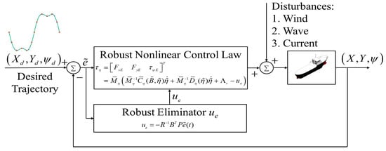
Figure 2.
The proposed control design for USVs considering modeling uncertainties and environmental disturbances.
In this investigation, we used two simulation scenarios to verify the trajectory-tracking performances of the proposed control method. Regarding comparisons between the proposed control laws (feedback linearization control law (FL) and robust feedback linearization control (RFL)), one modified sliding mode control (SMC) is derived by replacing the robust disturbance eliminator ue in (42) by , where ksmc is a designable control parameter. In the following section, brief descriptions of the controlled USV, modeling uncertainties caused by system parameters, and environmental disturbance-induced (wind, waves, and ocean currents) forces and torques will be introduced.
4.1. Specifications of the Controlled USV, Modeling Uncertainties and Environmental Disturbances

Table 2.
Specifications of the controlled USV.
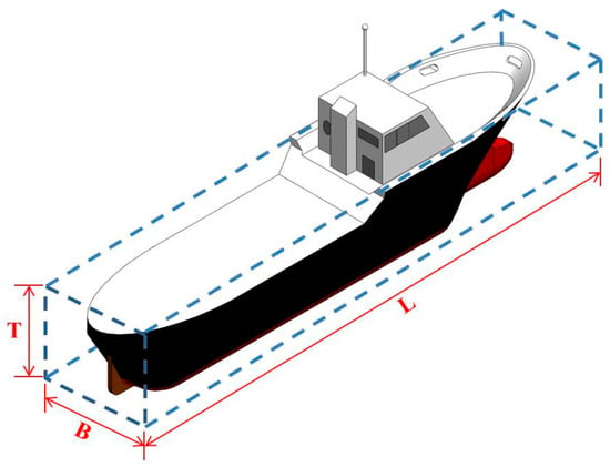
Figure 3.
Specifications of the controlled USV.
The system and environmental disturbance parameters for this controlled USV are as follows [14]:
where,
and
The modeling uncertainties of this USV were considered 10% of the inertial matrix M and the Coriolis and centripetal matrix C(v). Table 3 provides related parameters for simulating environmental disturbances (wind, waves, and ocean currents) [14].

Table 3.
Parameters for simulating environmental disturbances (wind, waves, and ocean currents).
Control parameters for FL, RFL, and the modified sliding mode control (SMC) [13] were assigned as follows:
The following parameters were chosen to construct the robust disturbance eliminator of the proposed robust control law:
P, which is optimally selected in section B, can be solved using the Riccati-like Equation (43) with the above A, B, Q, R and ρ = 0.6 as:
Regarding the designable control parameter ksmc of the SMC , we selected it as three to output similar control levels as the RFL and FL control methods.
4.2. Trajectory-Tracking Performance Verification with Respect to Different Attenuation Levels ρ
The robust performance index in (41) indicates that a lower attenuation level ρ will yield a better control performance under the effect of the overall external disturbance w. To fulfill the design objective expressed in (41), an attenuation level ρ between (0,1) is preferable. Solutions P in (43) for four different attenuation levels ρ = 0.6, 0.7, 0.8, and 0.9 are determined by solving the Riccati-like equation in (43). For comparison purposes, we deployed solutions P based on four attenuation levels (0.6, 0.7, 0.8, and 0.9) to construct the robust disturbance eliminator , observe the corresponding , and select an optimal attenuation level ρ. Figure 4 reveals the sailing trajectories of the controlled USV with respect to four attenuation levels ρ (0.6, 0.7, 0.8, and 0.9) under the effects of bound disturbances (modeling uncertainties and harsh environmental disturbances). Figure 5, Figure 6 and Figure 7 display the trajectory- and attitude-tracking errors of the X-axis, Y-axis, and ψ with respect to four attenuation levels ρ. Figure 8 shows the histories of the robust performance index in (41) with respect to four attenuation levels (ρ = 0.6, 0.7, 0.8, and 0.9). The enlarged part from 7 to 7.8 sec in Figure 4 indicates that the lower the attenuation level ρ is, the faster the convergence rate to the desired trajectory. The trajectory- and attitude-tracking errors in Figure 5, Figure 6 and Figure 7 also show that a lower attenuation level has smaller tracking errors in the X-axis, Y-axis, and heading angle ψ. Figure 8 shows the histories of the performance index with respect to the four attenuation levels (ρ = 0.6, 0.7, 0.8, and 0.9), indicating that a lower attenuation level consumes more energy at the beginning but less energy in the steady-state (about 10 to 57 s). Lower energy consumption and lower tracking error properties are maintained until the end due to the satisfactory trajectory- and attitude-tracking ability of the low attenuation level ρ = 0.6. Since RFL and its attenuation level ρ = 0.6 outperform the other designs (ρ = 0.7, 0.8, and 0.9), we compared it to the published FL in [17] for subsequent simulation scenarios.
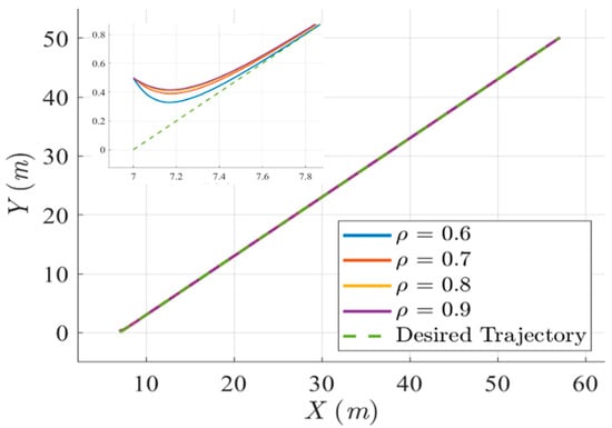
Figure 4.
Sailing trajectories of the controlled USV with respect to the desired trajectory of one ramp and four attenuation levels ρ = 0.6, 0.7, 0.8, and 0.9.
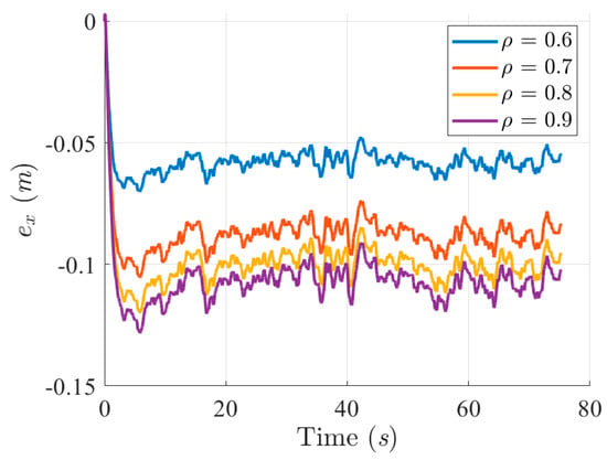
Figure 5.
Trajectory tracking errors in the X-axis with respect to four attenuation levels ρ = 0.6, 0.7, 0.8, and 0.9.
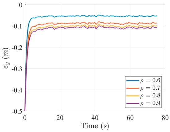
Figure 6.
Trajectory-tracking errors in the Y-axis with respect to four attenuation levels ρ = 0.6, 0.7, 0.8, and 0.9.
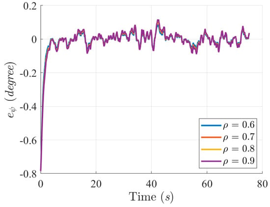
Figure 7.
Attitude-tracking errors of heading angles ψ with respect to four attenuation levels ρ = 0.6, 0.7, 0.8, and 0.9.
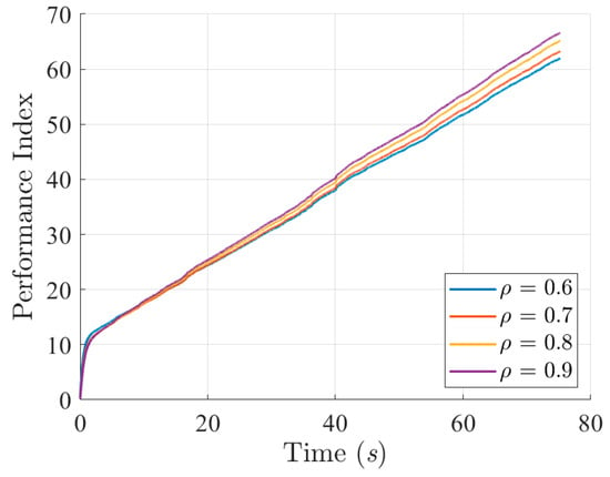
Figure 8.
Histories of the robust performance index in (41) with respect to four attenuation levels ρ = 0.6, 0.7, 0.8, and 0.9.
4.3. Scenario 1 (Ramp Trajectory)
In this scenario, a set of 11 waypoints listed in Table 4 are designated to the trajectory generator to generate a ramp trajectory. Table 5 shows the initial conditions of the controlled USV for this scenario.

Table 4.
Waypoints of Scenario 1.

Table 5.
Initial conditions for scenario 1.
Figure 9, Figure 10, Figure 11 and Figure 12 show the simulation results for tracking the desired ramp trajectory using the SMC, RFL, and FL control methods under the effects of bound modeling uncertainties and environmental disturbances. The proposed RFL control method shown in Figure 13, Figure 14 and Figure 15 has superior trajectory- and attitude-tracking performance than SMC and FL with the aid of the robust disturbance eliminator . Figure 16, Figure 17 and Figure 18 show that slightly bigger control commands (Fx, Fy and τψ), generated to eliminate modeling uncertainties and environmental disturbances and precisely guide the USV to follow the desired trajectory, can be achieved using the RFL method.
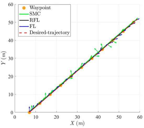
Figure 9.
Sailing trajectories and attitudes of the controlled USV based on SMC, RFL and FL control method for Scenario 1.
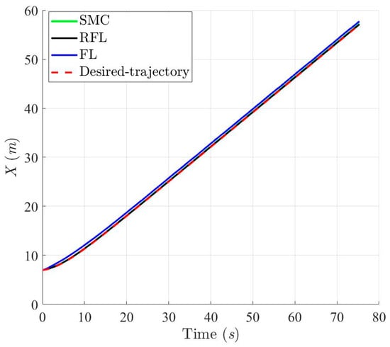
Figure 10.
Projection trajectories in X-axis with respect to SMC, RFL and FL method, respectively, for Scenario 1.
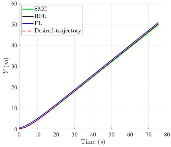
Figure 11.
Projection trajectories in Y-axis with respect to SMC, RFL and FL method, respectively, for Scenario 1.
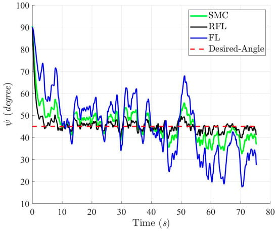
Figure 12.
Histories of heading angle ψ with respect to SMC, RFL and FL method, respectively, for Scenario 1.
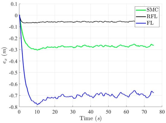
Figure 13.
Trajectory tracking errors in X-axis with respect to SMC, RFL and FL method, respectively, for Scenario 1.
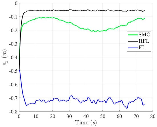
Figure 14.
Trajectory tracking errors in Y-axis with respect to SMC, RFL and FL method, respectively, for Scenario 1.
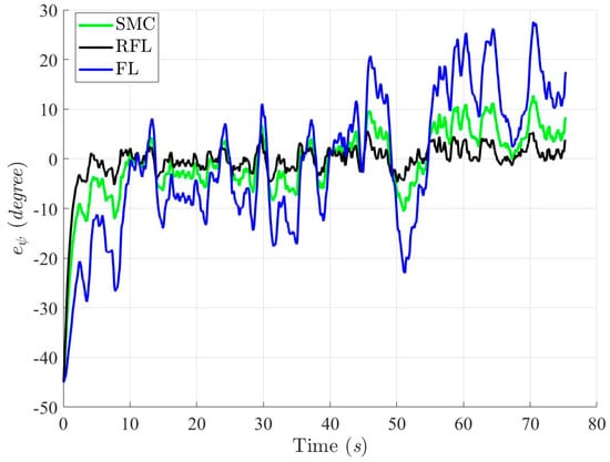
Figure 15.
Heading angle errors of ψ with respect to SMC, RFL and FL method, respectively, for Scenario 1.
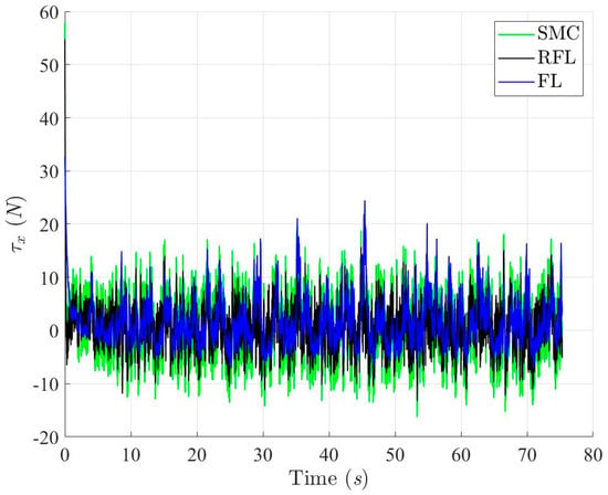
Figure 16.
Control Forces of the controlled USV in X-axis with respect to SMC, RFL and FL method, respectively, for Scenario 1.
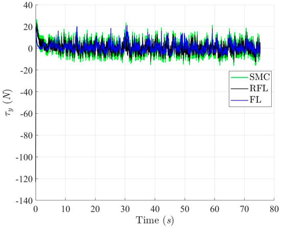
Figure 17.
Control Forces of the controlled USV in Y-axis with respect to SMC, RFL and FL method, respectively, for Scenario 1.
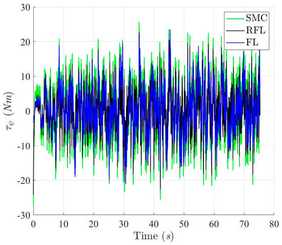
Figure 18.
Control torques of the controlled USV with respect to SMC, RFL and FL method, respectively, for Scenario 1.
4.4. Scenario 2 (U-Shaped Trajectory)
In this scenario, we assigned 19 waypoints to generate a U-shaped desired trajectory. Table 6 shows the waypoint set. Unlike the monotonic trajectory in Scenario 1, a sailing task with several turning points is assigned to the controlled USV using the SMC, RFL, and FL control methods in Scenario 2.

Table 6.
Waypoints of scenario 2.
Table 7 lists the initial conditions of the controlled USV for this scenario.

Table 7.
Initial conditions for scenario 2.
Figure 19, Figure 20, Figure 21 and Figure 22 show the simulation results of trajectories and attitudes for tracking the desired U-shaped trajectory with the SMC, RFL, and FL methods. Figure 23, Figure 24 and Figure 25 depict trajectory- and attitude-tracking errors based on the SMC, RFL, and FL control methods. Major tracking errors appeared in the simulation results for the SMC and FL control methods, whereas the RFL control method had minor ones. The RFL control method is immune to modeling uncertainties and environmental disturbances, resulting in minor but acceptable tracking errors. In Figure 19, Figure 22 and Figure 25, the USV heading angle ψ controlled by the SMC and FL control methods (green and blue arrow lines) varies considerably, especially at turning points. Due to modeling uncertainties and environmental disturbances, SMC and FL control methods cannot precisely direct the USV to follow a U-shaped trajectory. Conversely, the RFL control design was perfectly attached to the desired trajectory. The control forces and torques displayed in Figure 26, Figure 27 and Figure 28 indicate that the output torque of the proposed RFL control method was higher in the transient period than the SMC and FL control methods. In this case, the USV rapidly turned in the desired direction, and a suitable control torque was generated to accurately maintain this direction during the trajectory-tracking mission. Similarly, the proposed RFL control method outperformed the SMC and FL control methods in the trajectory and attitude-tracking performance of the USV in this complicated trajectory-tracking scenario. According to the simulation results described above, the RFL control method had nearly the same output level in control commands as the published SMC and FL control methods and delivered promising control performance to accurately guide USVs despite the effects of modeling uncertainties and environmental disturbances.
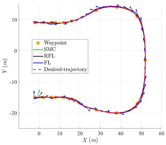
Figure 19.
Sailing trajectories and attitudes of the controlled USV based on SMC, RFL and FL control method for Scenario 2.
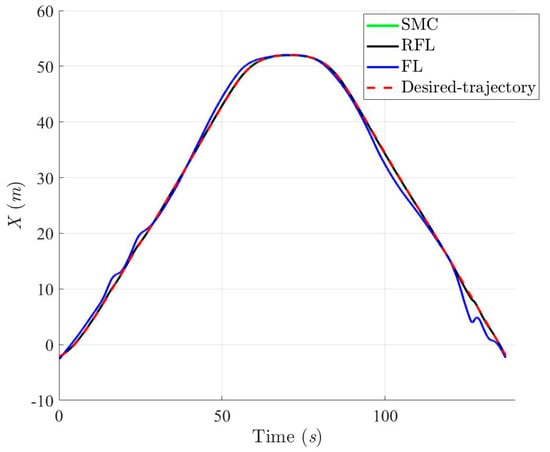
Figure 20.
Projection trajectories in X-axis based on SMC, RFL and FL control method for Scenario 2.
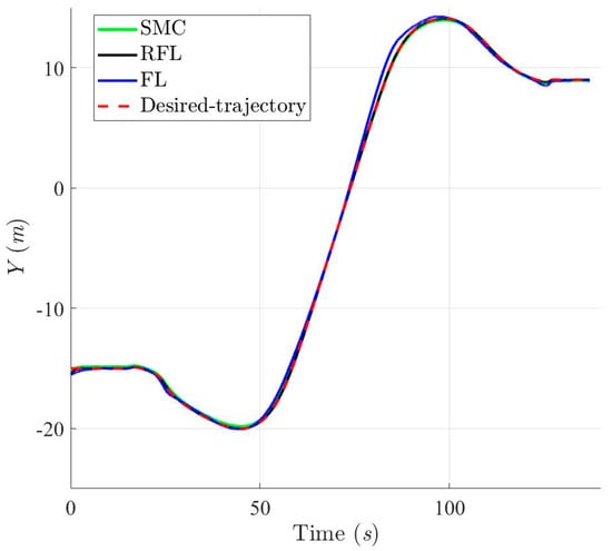
Figure 21.
Projection trajectories in Y-axis based on SMC, RFL and FL control method for Scenario 2.
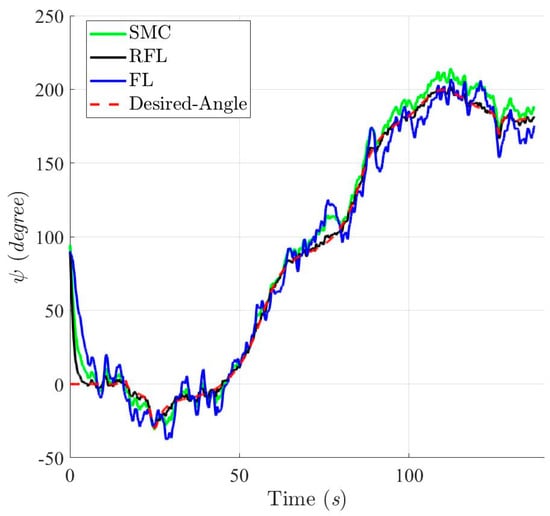
Figure 22.
Histories of heading angle ψ based on SMC, RFL and FL control method for Scenario 2.
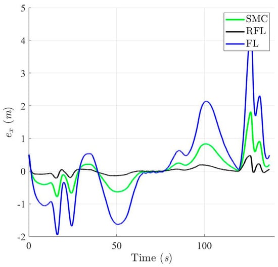
Figure 23.
Trajectory tracking errors in X-axis based on SMC, RFL and FL control method for Scenario 2.
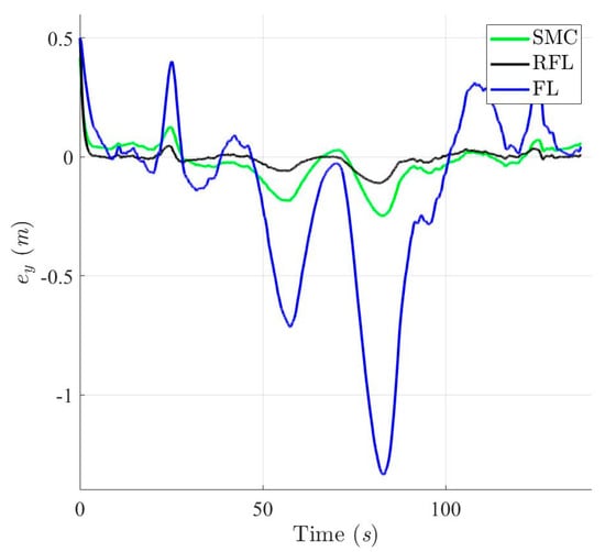
Figure 24.
Trajectory tracking errors in Y-axis based on SMC, RFL and FL control method for Scenario 2.
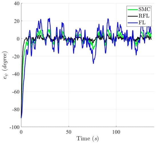
Figure 25.
Heading angle errors ψ based on SMC, RFL and FL control method for Scenario 2.
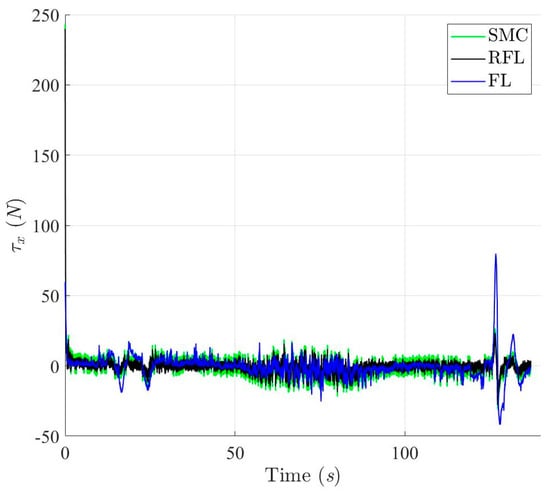
Figure 26.
Control Forces of the controlled USV in X-axis based on SMC, RFL and FL control method for Scenario 2.
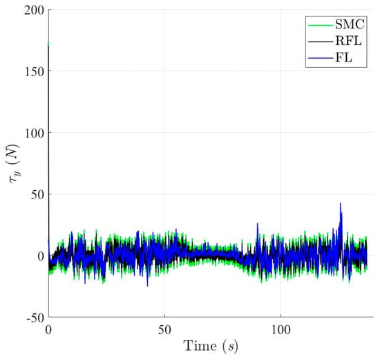
Figure 27.
Control Forces of the controlled USV in Y-axis based on SMC, RFL and FL control method for Scenario 2.
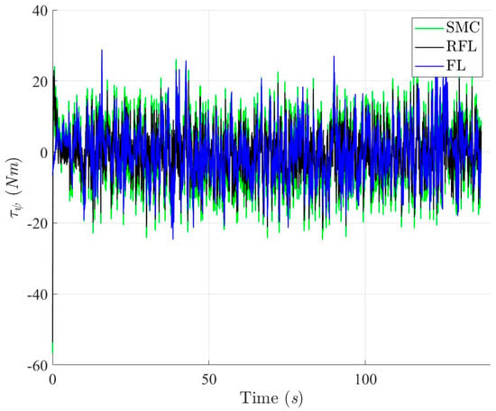
Figure 28.
Control torques of the controlled USV based on SMC, RFL and FL control method for Scenario 2.
5. Conclusions
We propose a nonlinear robust control design that integrates a feedback linearization control law and a robust disturbance eliminator to resolve trajectory tracking problems of unmanned surface vessels influenced by modeling uncertainties and environmental disturbances. In this investigation, we first transformed nonlinear error dynamics into a linear disturbed form using the feedback linearization control term of the proposed nonlinear robust control law. Then, we used the robust disturbance eliminator of the proposed control method to eliminate overall disturbances, including modeling certainties and environmental disturbances. Additionally, we verified the robustness of the controlled unmanned surface vessels’ closed-loop trajectory tracking system to overall disturbances. To analyze the trajectory tracking performance of this robust control method, a standard test trajectory was used in two comparative simulations: a ramp trajectory and a U-shaped trajectory, which is more complicated. According to the simulation results, our proposed control method outperforms the published feedback linearization control method in trajectory tracking accuracy, disturbance rejection, and control response. It delivers promising trajectory tracking performance for arbitrarily designed trajectories and handles the nonlinearities and modeling uncertainties of unmanned surface vessels and environmental disturbances well. Inherently, unmanned surface vessels installed with this proposed control method may play an important role in ocean rescue, ocean resources, hazardous terrain exploration, and other missions. In this investigation, we successfully developed a robust control scheme for the trajectory tracking of USVs. Several challenges must be overcome to achieve the experiment’s ultimate goal, including an analytical control allocation transformation between actuators and the desired robust control commands and the nonlinear relationship between the inputs and outputs of installed actuators. To the authors’ best knowledge, few studies have developed control systems for real USVs by integrating these subsystems (robust control law, control allocation, and mapping of actuators’ inputs and outputs).
Author Contributions
Conceptualization, Y.-H.C. (Yung-Hsiang Chen), Y.-Y.C. and G.-W.L.; methodology, Y.-H.C. (Yung-Hsiang Chen) and Y.-Y.C.; software, M.-Z.E.-T.,Y.-H.C. (Yu-Hsiang Chan) and G.-W.L.; validation, Y.-H.C. (Yung-Hsiang Chen) and Y.-Y.C.; formal analysis, Y.-H.C. (Yung-Hsiang Chen) and Y.-Y.C.; investigation, Y.-H.C. (Yung-Hsiang Chen), M.-Z.E.-T., Y.-H.C. (Yu-Hsiang Chan), G.-W.L. and Y.-Y.C.; resources, Y.-H.C. (Yung-Hsiang Chen) and Y.-Y.C.; data curation, M.-Z.E.-T.,Y.-H.C. (Yu-Hsiang Chan) and G.-W.L.; writing—original draft preparation, Y.-H.C. (Yung-Hsiang Chen) and Y.-Y.C.; writing—review and editing, Y.-H.C. (Yung-Hsiang Chen) and Y.-Y.C.; visualization, Y.-H.C. (Yung-Hsiang Chen), M.-Z.E.-T., Y.-H.C. (Yu-Hsiang Chan), G.-W.L. and Y.-Y.C.; supervision, Y.-H.C. (Yung-Hsiang Chen) and Y.-Y.C.; funding acquisition, Y.-H.C. (Yung-Hsiang Chen). All authors have read and agreed to the published version of the manuscript.
Funding
This research was funded by the MOST (Ministry of Science and Technology of Taiwan, project number is MOST 111-2221-E-020-023.
Institutional Review Board Statement
Not applicable.
Informed Consent Statement
Not applicable.
Data Availability Statement
Not applicable.
Conflicts of Interest
The authors declare no conflict of interest.
Appendix A
The following cost function refers to (41) prove Theorem 1, which is defined as:
This cost function can be further expressed as:
Substituting the linear-disturbed error dynamics in (40) into (A2), the following result can be obtained:
Equation (A3) can be further expressed as:
By applying (43) in
Theorem 1 and completing the square for (A4), we receive:
Using and in Theorem 1 yields
The inequality in (A6) is retained since and . Thus,
Therefore, if , this inequality reduces to the min–max tracking performance in (41) and Theorem 1 is proven.
References
- Protector Unmanned Surface Vehicle (USV). Available online: https://www.naval-technology.com/projects/protector-unmanned-surface-vehicle/ (accessed on 26 June 2013).
- Yara to Start Operating the World’s First Fully Emission-Free Container Ship. Available online: https://www.yara.com/corporate-releases/yara-to-start-operating-the-worlds-first-fully-emission-free-container-ship/ (accessed on 19 November 2021).
- Moradi, M.H.; Katebi, M.R. Predictive PID Control for Ship Autopilot Design. IFAC Proc. 2001, 34, 375–380. [Google Scholar] [CrossRef]
- Malecki, J. Applying of Fuzzy Logic to Precise Control of the Ship Motion. In Proceedings of the 2015 Second International Conference on Mathematics and Computers in Sciences and in Industry (MCSI), Sliema, Malta, 17 August 2015. [Google Scholar]
- Ahmed, Y.; Hasegawa, K. Fuzzy Reasoned Waypoint Controller for Automatic Ship Guidance. IFAC-PapersOnLine 2016, 49, 604–609. [Google Scholar] [CrossRef]
- Zhao, S.; Liu, S.; Keyser, R.; Ionescu, C.M. The Application of a New PID Autotuning Method for the Steam/Water Loop in Large Scale Ships. Processes 2020, 8, 196. [Google Scholar] [CrossRef]
- Du, J.; Hu, X.; Sun, Y. Adaptive Robust Nonlinear Control Design for Course Tracking of Ships Subject to External Disturbances and Input Saturation. IEEE Trans. Syst. Man Cyber. Syst. 2020, 50, 193–202. [Google Scholar] [CrossRef]
- Zwierzewicz, Z.; Dorobczyński, L.; Jaszczak, S. Design of Ship Course-keeping System via Active Disturbance Rejection Control Using a Full-scale Realistic Ship Model. Proc. Comp. Sci. 2021, 192, 3000–3009. [Google Scholar] [CrossRef]
- Dong, Z.; Bao, T.; Zhang, X.; Yang, L.; Song, L.; Mao, Y. Heading Control of Unmanned Marine Vehicles Based on an Improved Robust Adaptive Fuzzy Neural Network Control Algorithm. IEEE Access 2019, 7, 9704–9713. [Google Scholar] [CrossRef]
- Huang, Z.; Liu, X.; Wen, J.; Zhang, G.; Liu, Y. Adaptive Navigating Control Based on the Parallel Action-Network ADHDP Method for Unmanned Surface Vessel. Adv. Mat. Sci. Eng. 2019, 2019, 7697143. [Google Scholar] [CrossRef]
- Fan, Y.; Huang, H.; Tan, Y. Robust Adaptive Path Following Control of an Unmanned Surface Vessel Subject to Input Saturation and Uncertainties. Appl. Sci. 2019, 9, 1815. [Google Scholar] [CrossRef]
- Chen, Y.-Y.; Lee, C.-Y.; Tseng, S.-H.; Hu, W.-M. Nonlinear Optimal Control Law of Autonomous Unmanned Surface Vessels. Appl. Sci. 2020, 10, 1686. [Google Scholar] [CrossRef]
- Hsu, L.; Oliveira, T.R.; Cunha, J.P.V.S.; Yan, L. Adaptive Unit Vector Control of Multivariable Systems Using Monitoring Functions. Int. J. Robust Nonlinear Cont. 2019, 29, 583–600. [Google Scholar] [CrossRef]
- Fossen, T.I. Handbook of Marine Craft Hydrodynamics and Motion Control, 1st ed.; Wiley: New York, NY, USA, 2011; pp. 1–528. [Google Scholar]
- McKinley, S.; Levine, M. Cubic Spline Interpolation. Colle. Red. 1998, 45, 1049–1060. [Google Scholar]
- Chen, Y.-Y. Robust Terminal Guidance Law Design for Missiles Against Maneuvering Targets. Aero. Sci. Tech. 2016, 54, 198–207. [Google Scholar] [CrossRef]
- Chen, Y.-Y.; Fang, M.-C. Nonlinear Control Law Design of Unmanned Surface Vessels. J. Tw. Soc. Nav. Arch. Mar. Eng. 2013, 32, 83–89. [Google Scholar]
Disclaimer/Publisher’s Note: The statements, opinions and data contained in all publications are solely those of the individual author(s) and contributor(s) and not of MDPI and/or the editor(s). MDPI and/or the editor(s) disclaim responsibility for any injury to people or property resulting from any ideas, methods, instructions or products referred to in the content. |
© 2023 by the authors. Licensee MDPI, Basel, Switzerland. This article is an open access article distributed under the terms and conditions of the Creative Commons Attribution (CC BY) license (https://creativecommons.org/licenses/by/4.0/).