Article

BEM Turbine Model and PID Control System of a Floating Hybrid Wind and Current Turbines Integrated Generator System

Instituto de Automática e Informática Industrial ai2, Universitat Politècnica de València, Camino de Vera s/n, 46022 Valencia, Spain
*
Author to whom correspondence should be addressed.
J. Mar. Sci. Eng. 2023, 11(8), 1634; https://doi.org/10.3390/jmse11081634
Submission received: 10 July 2023 / Revised: 15 August 2023 / Accepted: 18 August 2023 / Published: 21 August 2023
(This article belongs to the Section Ocean Engineering)

Abstract

:
This is a new installment in the series of publications that describe the mathematical modeling of the Floating Hybrid Generator Systems Simulator (FHYGSYS) tool. This work presents an improved mathematical model of the turbines of the floating hybrid system—consisting of an “OC3-Hywind” wind turbine and two marine current turbines—presented by the authors in previous publications. In this third installment, the modeling of the three turbines of the floating hybrid system is described using the Blade Element Momentum (BEM) theory. This modeling allows one to replace the one based on the One-Dimensional theory used in previous installments. For the operation of modeling with BEM, it has been considered necessary to implement a continuous feedback control system. In this case, two PID (proportional–integral–derivative) controllers have been implemented in each of the turbines. The first controls the torque on the turbine generator and the second controls the collective pitch angle of the blades. The results obtained are presented and validated through a code-to-code comparison with simulations carried out with FASTv8 under the same conditions and with the operating results of marine current turbines that exist in the literature. This improvement in the mathematical model offers the possibility of implementing other types of controllers that allow for the testing of different strategies of the floating hybrid control system, with the aim of maximizing energy production while ensuring the structural stability of the floating hybrid system.

1. Introduction

To extract mechanical energy from a fluid, one of the most common options that has been used for centuries is the use of turbines [1]. Turbine modeling consists of finding a mathematical procedure that reproduces the real behavior of the turbine as accurately as possible. This modeling allows for the incorporation of turbines into simulation tools for mechanical systems such as FHYGSYS (Floating Hybrid Generator Systems Simulator).
Among the different turbine modeling techniques in the area of aerodynamics, two stand out: the One-Dimensional theory, also known Simple theory [2,3], and the Blade Element Momentum (BEM) theory [2,3,4]. The first is easier to implement and serves as a starting point for the application of the second. Turbine modeling using the One-Dimensional theory is based on reproducing the behavior of the turbine from known operating data, whether the data are from a real turbine or from proven precision simulators such as, for example, FASTv8 [5] and HAWC2 [6]. This makes it possible to easily reproduce the behavior of systems that incorporate turbines modeled with this technique.
However, turbine modeling using BEM provides results based on the mechanical and aerodynamic characteristics of the turbine, which allows one to predict the behavior of turbines for which real operating data have not been previously available.
Another important feature of turbine modeling using BEM is the following: by modifying the magnitudes of the turbine, which can be used as actuation magnitudes of a continuous feedback control system such as the generator torque or the pitch angle of the blades, results proportional to these modifications are obtained.
These two factors are the key that has motivated the implementation of turbine modeling using BEM in FHYGSYS, motivation that will be explained in detail and reasoned throughout this work.
Wind turbine modeling using BEM to compute turbine aerodynamics is widely used by many codes. In [7], some of the most relevant codes were analyzed, most of which used the BEM theory to model their wind turbines including most of the participants in Phase IV of the OC3 (Offshore Code Comparison Collaboration) project [8]. Likewise, BEM was also used by most of the participants of the OC4 [9], OC5 [10], and OC6 [11] projects.
In other works such as [12], the analytical, empirical, and computational methods for determining the aerodynamic forces on a single Horizontal Axis Wind Turbine (HAWT) have been reviewed. The application of BEM theory to a wind turbine is described in detail as well as the modeling of the wind and the application of both for the modeling of the aerodynamics of wind turbine farms.
In [13], a Real-Time Hybrid Simulation (RTHS) was presented that allowed the authors to generate data on the operation of Offshore Wind Turbines (OWT) in real-time, and combine these results with external equipment in the laboratory such as actuation and sensor systems. This work used the 5 MW reference wind turbine [14] from the National Renewable Energy Lab (NREL) installed on a monopile structure, implemented at different scales, and compared the RTHS data with those obtained in scaled real models. The modeling of the wind turbine was carried out using BEM theory in all cases.
The modeling of a 15 MW offshore wind turbine mounted on a fixed base was presented in [15], who used BEM theory for the aerodynamic modeling of the turbine. This work presented a model on a 1:70 scale that allowed the authors to obtain data for comparison with the modeling developed, in which the aero-elastic effects were not included. The wind turbine control system consisted of two parts: the generator torque controller and the collective blade pitch angle controller.
In another work (e.g., [16]), the validation techniques of BEM theory for the modeling of wind turbines were reviewed. These were fundamentally based on comparing the results obtained through turbine modeling using BEM theory with data from real wind turbines, or data obtained through Computational Fluid Dynamics (CFD) codes.
An interesting recent work was presented in [17], in which an extensive review of wind turbine aerodynamics modeling was carried out. Chapter 3 reviewed the wind turbine modeling using BEM theory, while Chapters 4 and 5 reviewed the CFD techniques applied to wind turbines. In Chapter 6, the aeroelastic effects on wind turbines were reviewed, and in Chapter 8, the consistency between different types of modeling was compared.
In [18], a study was carried out to improve the starting behavior of small HAWT at low wind speeds, a situation in which the low torque may not be enough to overcome the inertia of the turbine and therefore start the wind turbine. The BEM theory was used to model the wind turbine and the validation of the results was carried out with experimental data.
An aero-hydro-elastic model was described in [19] to predict the behavior of a floating OC3-Hywind-type wind turbine [14,20]. The aerodynamic modeling of the turbine was performed using BEM theory by comparing the results with those presented in [21].
Based on the current trend of increasing the diameters of wind turbines to obtain more energy, [22] explained the relationship between this increase and a greater flexibility of the wind turbine blades. This forces the simulators to be able to reproduce this behavior. This increase in flexibility was in contrast to many of the assumptions on which methods such as BEM theory are based. The work compared the results obtained with three different techniques: the first used OpenFAST [23] with BEM theory, the second also used OpenFAST but in this case a free vortex wake model—cOnvecting LAgrangian Filaments (OLAF)—was used to compute the aerodynamic forces on moving HAWT blades. The third technique used a high-fidelity CFD simulation software called Simulator for Wind Farm Applications (SOWFA). The study concluded that the three techniques agreed well for steady inflow conditions with no yaw misalignment, but that with increasing absolute yaw misalignment, the BEM results deviated significantly more from the SOWFA results.
Regarding research works on marine turbines, the study presented in [24] covered all of the issues of the simulation of marine turbines, from the modeling of the marine currents for long periods of time to the modeling of the marine turbines by applying the BEM theory. The results were compared with those presented in [25,26].
In [27], three scale-model tidal turbines were designed and arranged to form an array, thus obtaining experimental results of the interaction between each of the turbines. This work is complemented by [28], in which the modeling of the turbines was carried out using BEM theory and the ANSYS Fluent [29] CFD software, thus allowing for a comparison of the results between both works.
BEM theory was used in [30] for the modeling of two different concepts of marine turbines: a marine turbine with three blades of horizontal axis and a high solidity ducted and open-center turbine. The results were compared with various validation data from the literature.
Another example was shown in [31], in which BEM theory was used to model several tidal turbines that constituted a farm, specifically to a small cluster of ten turbines. Some simplifications were applied in this work such as considering each turbine as a disk to which a uniform fluid velocity was applied throughout the area swept by the turbines. The modeling of the fluid that interacted with each of the tidal turbines was carried out using SHYFEM (System of HydrodYnamic Finite Element Modules) [32], validating the model from the experimental data.
Finishing this brief review, in [33]. a model of tidal turbines in a water–sediment environment was presented. Once again, the authors used BEM for the modeling of the turbines, but corrected the values of the lift coefficient (CL) and the drag coefficient (CD) of each airfoil. The fluid modeling was performed with ANSYS Fluent [29], and they compared the results with the experimental data obtained in a wind tunnel.
Focusing on the present work, this article presents the way in which the two types of turbines—wind and marine current turbines (MCT)—have been modeled using BEM in a floating hybrid system, like the one shown in Figure 1.
Both the wind turbine and the two MCTs are part of the floating hybrid system, so in order to obtain results for their study and validation, it is necessary to have an adequate mathematical model of the system as a whole and of the environment—seawater—in which it is found. A complete mathematical model of the floating hybrid system shown in Figure 1—consisting of a floating OC3-Hywind-type wind turbine [14,20] to which two MCTs have been coupled such as those described in [34,35]—was presented in [36,37], but without using the BEM theory for the modeling of the turbines. The complete mathematical model was implemented in [36,37] using MATLAB®, and they called the resulting code FHYGSYS. In [36], the kinematic, dynamic, and inertial models were presented and the way in which the added mass of the floating system was computed. On the other hand, in [37], the method to calculate the hydrodynamics and the rest of the forces acting on the floating hybrid system was described in detail including the modeling of the turbines using One-Dimensional theory.
In this third installment, the mathematical modeling presented in [36,37] is extended, offering the possibility to choose between the One-Dimensional theory or the BEM theory for turbine modeling in FHYGSYS. In this case, the programming environment used was also MATLAB®. From the point of view of computing time, the simulation of the three turbines of the floating hybrid system using the BEM theory was longer than using One-Dimensional theory. However, from the point of view of the quality of the modeling of the turbines, the use of BEM theory offers significant improvements.
With One-Dimensional theory, the turbine is modeled as a disk on which the fluid impinges homogeneously [2,3]—generating a thrust on the turbine—considering constant the fluid velocity over the area swept by the turbine disc, with the results being independent of the number of blades it has. For this reason, as discussed in previous paragraphs, turbine operating data are needed to reproduce its behavior, and it is not possible to infer results from turbines for which the operating data are not known.
On the contrary, the BEM theory is implemented by dividing each of the turbine blades into portions—called blade elements (see Figure 1)—that are assigned a different geometry and airfoil [2,3,4] (or hydrofoil). In this case, it is considered that the fluid impinges on each blade element (with a different fluid velocity, depending on the height or depth), generating a thrust on the turbine from the thrust originating in each of the blade elements, thus obtaining results without the prior knowledge of turbine operating data.
Strictly speaking, the experimental operating data must be known, but not on the operation of the turbine, but rather on the behavior of the airfoils or hydrofoils that are usually obtained in wind tunnels. As indicated in [38], the behavior of hydrofoils in water is analogous to the behavior of airfoils in air, the main difference between them being the fluid density. This allows for the use of the experimental data from airfoils in the modeling of marine turbines.
After consulting the existing literature, BEM theory is applied in essentially the same way, but the application in this work was based on the methodology used in [2,3,4], with some differences that will be explained in detail in the following sections. In the same way as in [15], the aero-elastic effects were not included, and the turbine control consisted of two parts: a generator torque controller and a collective blade pitch angle controller.
In summary, with the inclusion of the BEM theory, a more precise turbine modeling is obtained and, in addition, two fundamental objectives are achieved: the first one is to provide two acting magnitudes on the floating hybrid system in each of the turbines—the generator torque and the blade pitch angle—that allow for the testing of different control strategies on it [39]. The second is to present a model that allows us to obtain the results of turbines for which the operating data are not previously known.
The rest of this paper is structured as follows. Section 2.1 explains how BEM theory is used in FHYGSYS for turbine modeling. In Section 2.2, we explain in detail how BEM theory is applied in FHYGSYS. Next, in Section 2.3, the calculation of the magnitudes of the wind turbine obtained from the application of BEM theory is described and in Section 2.4, the control system implemented in the wind turbine is presented. Then, in Section 2.5, the differences and similarities between the calculation of the magnitudes of the wind and MCTs obtained from the application of the BEM theory are indicated, and in Section 2.6, the control system implemented in MCTs is described. Section 3 explains the results obtained in the performed tests, and finally, Section 4 presents the discussion and future work for this line of research.

2. Materials and Methods

2.1. Introduction to Turbine Modeling Using Blade Element Momentum Theory

The application of BEM theory in FHYGSYS is illustrated in Figure 2. It shows how the modeling of turbine aerodynamics, or hydrodynamics in the case of MCTs, using BEM theory is related to the rest of the mathematical model of the floating hybrid system.
The first step for the application of this method in FHYGSYS is the calculation of the effective fluid velocity vector in each blade element (see Figure 2) by applying the methodology described in Section 2.3 in [37]. In this way, a different fluid velocity is obtained for each blade element, which offers an adequate approximation to the real behavior, since the differences in height or depth can be considerable in the turbine blades.
From the effective fluid velocity vector calculated in each blade element, a calculation algorithm from the BEM theory is applied (see Figure 2); specifically in this work, the one described in [2] was chosen. This algorithm includes some corrections that are presented in the next section. From the application of the BEM algorithm, three fundamental magnitudes are obtained for each blade element: the differential of thrust force ( d F t h r u s t ), the differential of torque force ( d F t o r q u e ), and the differential of pitching moment ( d M p i t c h i n g ). These are the quantities from which the rest of the turbine modeling calculations in FHYGSYS are deduced, calculations that are described in the following sections.
Once the BEM algorithm has been applied to the blade elements of each of the turbine blades, the results are integrated, obtaining the values of F t h r u s t , F t o r q u e , and M p i t c h i n g of the turbine. These values are used, on the one hand, to obtain the new angular position of the turbine, and on the other hand, to contribute to the acceleration of the floating hybrid system by acting on its dynamics (see Figure 2). This process is repeated for the new angular position of the turbine until the end of the simulation.

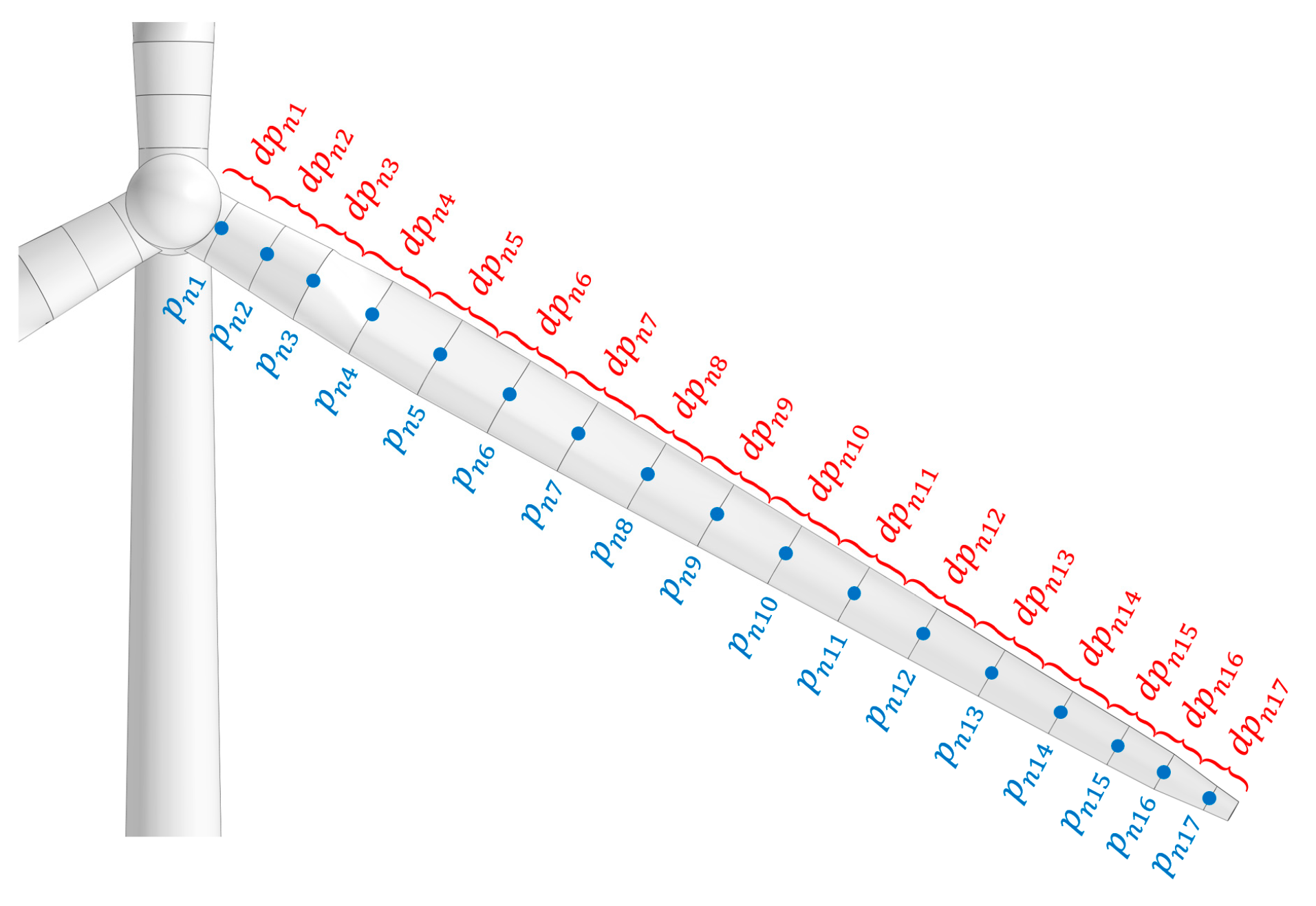
2.2. Application of Blade Element Momentum Theory

For clarity in the study, in this section, the application of BEM theory is explained using the wind turbine as an example. In Section 2.5, the differences and similarities in the application of the BEM theory between the wind and the MCTs are discussed.
As indicated in the preceding sections, the previous step to the application of BEM theory is the division of the blades into blade elements or blade differentials ( d p n i ). Figure 3 shows this division made in one of the blades of the wind turbine. In this work, the center of each of the blade elements is called p n i . The values of the p n i points of each of the blades of the wind and MCTs can be found in Appendix A, expressed in a blade coordinate system ( p n i ( B L A D E ) ) and in the mobile coordinate system ( p n i ( B O D Y ) ).
Each blade was divided into 17 blade elements for consistency with [14] and because it has been verified that dividing the blade into a greater number of blade elements does not offer significant differences in the results obtained, but increases the simulation computing time.
As shown in Figure 2 and as indicated in the previous section, the first step to applying BEM theory in FHYGSYS is the calculation of the effective fluid velocity vector—the effective wind velocity vector in this case—at the center point ( p n i ) of each blade element, which is based in the methodology described in Section 2.3.1 in [37], but including a correction that considers the tower shadow effect. This calculation starts from the data found in Appendix A, expressing the p n i   ( B O D Y ) ( t ) points in the inertial coordinate system using Equation (1), in which the homogeneous transformation matrix M H T B O D Y I N E R T I A L appears. The calculation of this matrix is explained in detail in Section 2.3.1 in [36].
p n i   ( I N E R T I A L ) ( t ) = M H T B O D Y I N E R T I A L · p n i   ( B O D Y ) ( t )
Because the floating hybrid system is subject to displacements and rotations in a Euclidean space (see Figure 1), to calculate the effective wind velocity vector, the velocity vector ( v   p n i   ( B O D Y ) ( t ) ) of the center point ( p n i ) of each blade element must be known. This is achieved in two steps: calculating with Equation (2) the derivative with respect to time by applying the Richardson extrapolation method [40] (as shown in Appendix C in [36]) of each of these points expressed in the inertial coordinate system ( p n i   ( I N E R T I A L ) ( t ) ) and with Equation (3), expressing this velocity vector in the mobile coordinate system.
v   p n i   ( I N E R T I A L ) ( t ) = d d t   p n i   ( I N E R T I A L ) ( t )
v   p n i   ( B O D Y ) ( t ) = ( M B O D Y I N E R T I A L ) 1 · v   p n i   ( I N E R T I A L ) ( t )
As indicated in [37], the M B O D Y I N E R T I A L matrix of Equation (3) is equivalent to the M H T B O D Y I N E R T I A L matrix of Equation (1). With the M B O D Y I N E R T I A L matrix, the vectors are represented with three components, while with the M H T B O D Y I N E R T I A L matrix, they must be represented in a homogeneous format. Next, the wind speed ( V W I N D ( h ) ) at the height of the center point of each blade element ( p n i ) is calculated from the wind speed ( V W R E F ) at the reference height ( z R E F ) using Equation (4), extracted from [41]. The reference height ( z R E F ) is 90 m above the still water level (the height of the hub of the wind turbine in the initial position [14,20]) following the same criteria used in [5,41]. The z W I N D ( t ) height is the Z component of the p n i points expressed in the inertial coordinate system ( p n i ( I N E R T I A L ) ( t ) ), and α is the power law exponent, which has a value of 1/7 for normal wind conditions [41].
V W I N D ( h ) = V W R E F · ( z W I N D ( t ) z R E F ) α
The wind velocity vector expressed in the inertial coordinate system can be obtained with Equation (5), where δ is the angle that represents the wind direction. Through Equation (6), this vector can be found, but is expressed in the mobile coordinate system ( v   W I N D   ( B O D Y ) ( h ) ).
v   W I N D   ( I N E R T I A L ) ( h ) = V W I N D ( h ) · [ cos δ sin δ 0 sin δ cos δ 0 0 0 1 ] · [ 1 0 0 ]
v   W I N D   ( B O D Y ) ( h ) = ( M B O D Y I N E R T I A L ) 1 · v   W I N D   ( I N E R T I A L ) ( h )
To finish the calculation of the effective wind velocity vector, a correction is carried out that considers the tower shadow effect. While there are different techniques in the literature, out of all of them, the correctiSon presented in [4] was chosen. To apply this correction, the center point of each blade element is expressed according to Equation (7).
[ x p n i y p n i z p n i ] = [ cos ( δ ) sin ( δ ) 0 sin ( δ ) cos ( δ ) 0 0 0 1 ] · p n i   ( B O D Y ) ( t )
From the results of Equations (6) and (7), through Equation (8) (extracted from [4]), the wind velocity vector ( v   W I N D   t o w e r s h a d o w   ( B O D Y ) ( h ) ) can be obtained considering the tower shadow effect.
v   W I N D   t o w e r s h a d o w     ( B O D Y ) ( h ) = v   W I N D   ( B O D Y ) ( h ) · ( 1 ( D ( h ) 2 ) 2 · ( x p n i 2 y p n i 2 ) ( x p n i 2 + y p n i 2 ) 2 )
The diameter D ( h ) of Equation (8) can be calculated by performing linear interpolation from the data in Table 1 and the value of the Z component of the p n i points expressed in the mobile coordinate system ( z p n i ) when these are less than the value of hTower−top.
As shown in Figure 4, the central points of each blade element in Equation (7) can be considered as expressed in the tower shadow coordinate system since this system matches that of the mobile coordinate system. Additionally, in Figure 4, the tower shadow calculation zone can be observed; this is the zone in which Equation (8) is applied.
Therefore, the calculation of the effective wind velocity vector ( v   n i   E F F W I N D ( B O D Y ) ( h , t ) ) can be undertaken through Equations (9) and (10) by using Equation (9) if the center point of each blade element ( p n i ) is outside the tower shadow calculation zone, and using Equation (10) if otherwise. However, it should be kept in mind that Equation (10) only applies if the following condition is true: | v   W I N D   t o w e r s h a d o w   ( B O D Y ) ( h ) | < | v   W I N D   ( B O D Y ) ( h ) | .
v   n i   E F F W I N D   ( B O D Y ) ( h , t ) = v   W I N D   ( B O D Y ) ( h ) + v   p n i   ( B O D Y ) ( t )
v   n i   E F F W I N D   ( B O D Y ) ( h , t ) = v   W I N D   t o w e r s h a d o w     ( B O D Y ) ( h ) + v   p n i   ( B O D Y ) ( t )
The next step is the reasoning of how the effective wind velocity vector acts on each of the turbine blades. Obviously, this vector is not aligned with the blades for different reasons including the shaft tilt angle, the movement of the floating system due to buoyancy, sea currents, the waves, etc. The modeling of this situation is carried out in a similar way to that described in Section 2.8.1 in [37]. In this case, the projection vector [42] of the effective wind velocity vector ( v   n i   E F F W I N D   ( B O D Y ) ( h , t ) ) is calculated over the unit vector perpendicular to each of the blades ( u   B j   t h r u s t   ( B O D Y ) ). This is calculated using Equation (11), and the symbol * in the equation means the scalar product of the two vectors.
v   n i   E F F B j   t h r u s t   ( B O D Y ) ( t ) = u   B j   t h r u s t   ( B O D Y ) · v   n i   E F F W I N D   ( B O D Y ) ( h , t ) * u   B j   t h r u s t   ( B O D Y ) | u   B j   t h r u s t   ( B O D Y ) | 2
V 0 ( t ) = V 0   i j ( t ) = | v   n i   E F F B j   t h r u s t ( B O D Y ) ( t ) |
The magnitude of the effective wind velocity vector ( v   n i   E F F B j   t h r u s t ( B O D Y ) ( t ) ) on each of the blades obtained in Equation (11) is named as either V 0 ( t ) or V 0   i j ( t ) in Equation (12) for simplicity in subsequent calculations and for consistency with the nomenclature used in [3]. Figure 5 shows the unit vectors ( u   B j   t h r u s t ) perpendicular to each of the blades. The calculation of these vectors can be found in Appendix A.

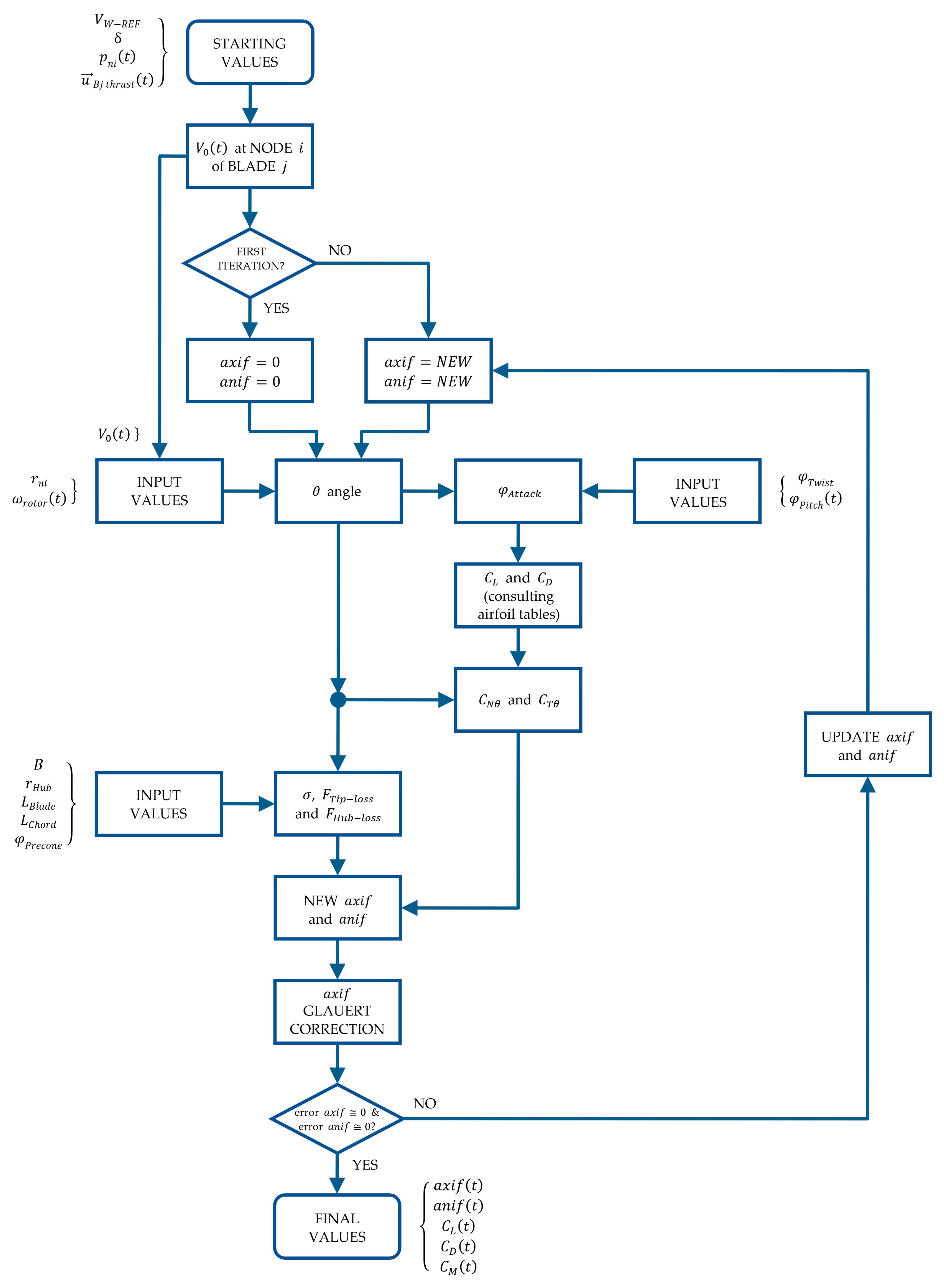
2.2.1. BEM Algorithm Application

The application of the BEM algorithm starts from the magnitude ( V 0 ( t ) ) obtained with Equation (12). In addition to this important value, it is necessary to know the properties that define the wind turbine, which were extracted from [14] and appear in Table 2.
Figure 6 shows the algorithm used in FHYGSYS for the application of the BEM theory. This algorithm is based on the one explained in [2], and the equations that compose it are presented below.
For the application of this algorithm, it is also necessary to know the aerodynamic properties of the wind turbine blades, which were extracted from [14] and are shown in Table 3.
The aerodynamic properties of the wind turbine blade that appear in Table 3 are the same as those described in [14], since the floating hybrid system is based on the “OC3-Hywind” concept, except for the twist angle of nodes 1, 2, and 3. As the airfoil of these nodes is a cylinder, these twist angles were set to zero.
The algorithm in Figure 6 starts from the value of V 0 ( t ) , then by applying Equations (13) and (14)—extracted from [2,3,4]—the normal ( V 1 2 ( t ) ) and tangential ( V r o t ( t ) ) velocities to the vertical plane of each blade can be obtained. The value of r n i was taken from Table 3 for each blade element (see Figure 4) and the low-speed shaft angular speed of the turbine ω r o t o r ( t ) = 0 for the initial time instant of the simulation ( t = 0 ). As seen in Figure 6, the values of a x i f ( t ) and a n i f ( t ) equaled zero at the beginning of the iterations each time the algorithm was applied.
V 1 2 ( t ) = V 0 ( t ) · ( 1 a x i f ( t ) )
V r o t ( t ) = ω r o t o r ( t ) · r n i · ( 1 + a n i f ( t ) )
Figure 7 is based on the explanation of aerodynamics from [3] and represents how aerodynamics (or hydrodynamics) is applied to each blade element in FHYGSYS.
Following the reasoning presented in [2,3,4], the magnitude of the wind velocity reaching each blade element ( V r e l ( t ) ) and the angle between this velocity and the vertical plane of each blade ( θ ( t ) ) can be calculated using Equations (15) and (16).
V r e l ( t ) = V r o t 2 ( t ) + V 1 2 2 ( t )
θ ( t ) = atan V 1 2 ( t ) V r o t ( t )
Figure 7 shows the relationship between Equations (13)–(16), with Equations (15) and (16) being the result of applying trigonometry to the results of Equations (13) and (14). From the θ ( t ) angle, the pitch angle of the blade ( φ P i t c h ( t ) )—which depends on the control system (see Section 2.4.2)—and the twist angle ( φ T w i s t ) of each blade element (see Table 3), the angle of attack ( φ A t t a c k ( t ) ) between the relative wind velocity ( V r e l ( t ) ) and the chord line of each blade element can be obtained (see Figure 7). This is expressed mathematically by Equation (17) and graphically in Figure 7.
φ A t t a c k ( t ) = θ ( t ) φ P i t c h ( t ) φ T w i s t
Expressing the angle of attack ( φ A t t a c k ( t ) ) in degrees, the airfoil-data tables corresponding to each blade element (see Table 3) were consulted to obtain the values of the lift coefficient ( C L ( t ) ), drag coefficient ( C D ( t ) ), and pitching-moment coefficient ( C M ( t ) ). The airfoil-data tables used for the wind turbine can be found in Appendix B in [14].
From the values of C L ( t ) and C D ( t ) , the values of the normal ( C N θ ( t ) ) and tangential ( C T θ ( t ) ) coefficients for the θ ( t ) angle are obtained by means of Equations (18) and (19). These equations were extracted from [2,4] and can also be deduced from [3].
C N θ ( t ) = C L ( t ) · cos ( θ ( t ) ) + C D ( t ) · sin ( θ ( t ) )
C T θ ( t ) = C L ( t ) · sin ( θ ( t ) ) C D ( t ) · cos ( θ ( t ) )
The next step is the calculation of the losses (tip and hub losses) in the wind turbine. As a previous step, the turbine radius ( r T u r b i n e ) is calculated using Equation (20); the data in this equation can be found in Table 2.
r T u r b i n e = ( L B l a d e + r H u b ) · cos ( φ P r e c o n e )
Tip-losses are modeled using Prandtl’s tip-loss factor ( F T i p l o s s ( t ) ), as shown in Equation (21), where B is the number of turbine blades (see Table 2). This model is widely used and can be found in [2,3,4,43].
F T i p l o s s ( t ) = 2 π · acos [ exp ( B · ( r T u r b i n e r n i ) 2 · r n i · sin θ ( t ) ) ]
The hub-losses are modeled through Equation (22) (extracted from [43]), thus obtaining the hub-loss factor (FHub−loss(t)). The total turbine losses ( F l o s s ( t ) ) are obtained by multiplying these two factors [43], as shown in Equation (23).
F H u b l o s s ( t ) = 2 π · acos [ exp ( B · ( r n i r H u b ) 2 · r n i · sin θ ( t ) ) ]
F l o s s ( t ) = F T i p l o s s ( t ) · F H u b l o s s ( t )
Next, a local solidity [2,3,4,43] is calculated with Equation (24), which is defined in [2] “as the fraction of the annular area in the control volume that is covered by the blades”. In this equation, the value of L C h o r d can be found in Table 3 and is illustrated in Figure 7.
σ i = B · L C h o r d 2 · π · r n i
From the local solidity ( σ i ), the new values of both the axial induction factor ( a x i f ( t ) ) and angular induction factor ( a n i f ( t ) ) are obtained. However, it must be taken into account that the application of BEM theory breaks down from values of a x i f ( t ) greater than 0.4 [2,4,43]. Therefore, it is common to include techniques—usually based on empirical data—to correct this situation. Two different techniques have been implemented in FHYGSYS to solve this issue: the Glauert correction [2,4,43] and the Wilson and Walker correction [2]. Although both types of correction can be used in FHYGYS, all of the simulations presented in this work were performed using the Glauert correction.
For clarity, in the equation that yields a x i f ( t ) , the term K a x i f ( t ) (also used in [2]) has been previously calculated with Equation (25).
K a x i f ( t ) = 4 · F l o s s ( t ) · sin 2 ( θ ( t ) ) σ i · C N θ ( t )
Thus, the calculation of the a x i f ( t ) is obtained through Equation (26) in a simpler way, where a x i f m a x is the threshold for the application of the correction when the BEM theory breaks down. Equation (25) is taken from [2] and Equation (26) is deduced from the equation for calculating the a x i f ( t ) also presented in [2].
a x i f ( t ) = 1 K a x i f ( t ) + 1         f o r   a x i f ( t ) a x i f m a x
The application of the Glauert correction [2,4,43] is based only on the application of an equation. In FHYSGYS, this equation is deduced by applying the same reasoning presented in [2] for the Wilson and Walker correction, but using the equation for the Glauert correction also described in [2]. This option was chosen because, after carrying out some tests with the methods presented by various authors, this has been the method in which the best results have been obtained in the process of validating the mathematical model of the wind turbine with FASTv8. To apply the Glauert correction, two equations can be used: Equation (27), which is the result of applying the criteria described, or its polynomial version, according to K a x i f ( t ) , as shown by Equation (28), which is the one used in FHYGSYS.
4 · a x i f ( t ) · ( 1 1 4 · ( 5 3 · a x i f ( t ) ) · a x i f ( t ) ) · F l o s s ( t ) = ( 1 a x i f ( t ) ) 2 · σ i · C N θ ( t ) sin 2 ( θ ( t ) )
3 4 · K a x i f ( t ) · a x i f 3 ( t ) ( 5 4 · K a x i f ( t ) + 1 ) · a x i f 2 ( t ) + ( K a x i f ( t ) + 2 ) · a x i f ( t ) 1 = 0
As indicated in [2], the value of a x i f m a x for the Glauert correction is 1/3, therefore, to apply this correction, when the value of a x i f ( t ) obtained with Equation (26) exceeds this value ( a x i f m a x > 1 / 3 ), it is recalculated by applying Equation (28). This equation is solved in FHYGSYS by applying the Newton–Raphson method described in [40].
As previously indicated, the a n i f ( t ) calculation is also obtained from the local solidity ( σ i ). By analogy with the previous case—as a step prior to calculating the a n i f ( t ) —the K a n i f ( t ) value is obtained using Equation (29), this allows one to express the obtaining of the a n i f ( t ) value more clearly through Equation (30). Equations (29) and (30) are deduced from the equation for calculating the a n i f ( t ) presented in [2].
K a n i f ( t ) = 4 · F l o s s ( t ) · sin ( θ ( t ) ) · cos ( θ ( t ) ) σ i · C T θ ( t )
a n i f ( t ) = 1 K a n i f ( t ) 1
For the BEM algorithm (see Figure 6) to be executed, a singularity is produced in the value of a n i f ( t ) in the first instants of time of the simulation, when the turbine has an angular speed close to zero. This singularity is avoided by forcing the value of a n i f ( t ) not to take values less than −1. This is expressed mathematically in Equation (31).
a n i f ( t ) = 1           f o r   a n i f ( t ) < 1
Equations (13)–(31) represent a loop in which the values of a x i f ( t ) and a n i f ( t ) are calculated, and consequently the values of the rest of the magnitudes are set by iteration (see Figure 6). The iteration stops when the value of the percent relative error ( ε a ) of these two values— a x i f ( t ) and a n i f ( t ) — is less than a chosen threshold ( ε a < ε a m i n ). The minimum value of the percent relative error ( ε a m i n ) used in FHYGSYS for this iteration is ε a m i n = 5 · 10 9 . The formula used to calculate these errors is shown in Equation (32), which corresponds to the one to calculate the percent relative error ( ε a ) indicated in [40]. In Equation (32), c u r r e n t   v a l u e are those calculated by means of Equations (26) and (30) and p r e v i o u s   v a l u e are those included in Equations (13) and (14), according to the calculation of the percent relative error of a x i f ( t ) or a n i f ( t ) , respectively, considering that the a x i f ( t ) value of Equation (26) can be recalculated by Equation (28), as explained above.
ε a = c u r r e n t   v a l u e p r e v i o u s   v a l u e c u r r e n t   v a l u e · 100

2.3. Obtaining Values of the Wind Turbine Magnitudes

The BEM algorithm shown in Figure 6 and explained in the previous section, was applied to each blade element for each of the wind turbine blades. Figure 8 shows the relationship between the BEM algorithm and the rest of the actions for the calculation of the main magnitudes of the wind turbine at a given simulation time instant.
These main magnitudes are the differential rotor thrust force ( d F t h r u s t ), the differential rotor torque force ( d F t o r q u e ), and the differential pitching moment ( d M p i t c h i n g ). From them, the calculation of the vector of wind turbine forces, the moment about the shaft, the blade azimuth position, and other additional magnitudes of the wind turbine can be derived. The reasoned deduction for all of them is discussed in the following subsections.

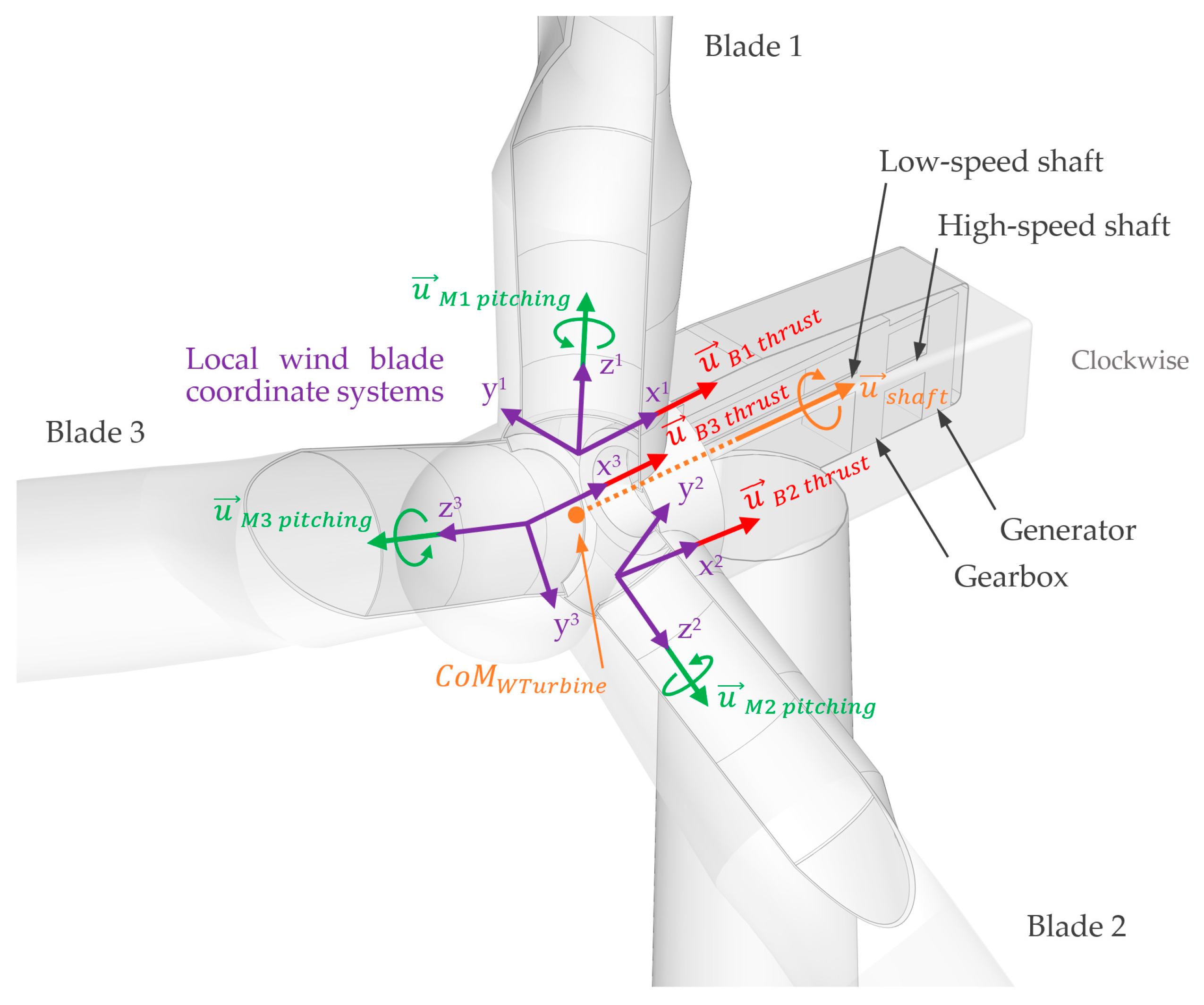
2.3.1. Moment about the Shaft

From the data calculated in the blade elements ( i ) of each of the blades ( j )—fundamentally from C L ( t ) , C D ( t ) and C M ( t ) —the main magnitudes shown in Figure 8 can be calculated. Using Equations (33) and (34)—based on the explanations of [3]—the values of the differential rotor thrust force ( d F t h r u s t   i j ( t ) ) and differential rotor torque force ( d F t o r q u e   i j ( t ) ) in the blade elements of each of the wind turbine blades can be calculated.
d F t h r u s t   i j ( t ) = 1 2 · ρ A I R · V r e l   i 2 ( t ) · L C h o r d   i · C N θ   i ( t ) · d p n i
d F t o r q u e   i j ( t ) = 1 2 · ρ A I R · V r e l   i 2 ( t ) · L C h o r d   i · C T θ   i ( t ) · d p n i
In [3], Equation (33) appears multiplied by the number of blades ( B ), but in FHYGSYS, Equation (33) is applied to each blade element of each of the blades independently, later adding the effect of each of them, considering a different wind vector affecting the blade elements depending on the height, as already explained in previous sections. On the other hand, Equation (34) is the one expressed in [3] for the calculation of the differential rotor torque but omitting the radius, thus obtaining the differential force that produces the differential rotor torque indicated in [3].
With this approach, the differential rotor thrust force ( d F   t h r u s t   i j   ( B O D Y ) ( t ) ) and differential rotor torque force ( d F   t o r q u e   i j   ( B O D Y ) ( t ) ) vectors can be found by applying Equations (35) and (36), multiplying by the unit vectors ( u   B j   t h r u s t   ( B O D Y ) and u   B j   t o r q u e   ( B O D Y ) ) the values obtained in Equations (33) and (34), respectively. These unit vectors may be observed—or reasoned—from Figure 5 and Figure 7, and their values appear in Appendix A.
d F   t h r u s t   i j   ( B O D Y ) ( t ) = d F t h r u s t   i j ( t ) · u   B j   t h r u s t   ( B O D Y )
d F   t o r q u e   i j   ( B O D Y ) ( t ) = d F t o r q u e   i j ( t ) · u   B j   t o r q u e   ( B O D Y )
Next, using Equation (37), the resultant ( d F   b l a d e   i j   ( B O D Y ) ( t ) ) of the differential forces calculated with Equations (35) and (36) is obtained (see Figure 7).
d F   b l a d e   i j   ( B O D Y ) ( t ) = d F   t h r u s t   i j   ( B O D Y ) ( t ) + d F   t o r q u e   i j   ( B O D Y ) ( t )
The next step is to calculate the differential moments ( d M   b l a d e   i j   ( B O D Y ) ( t ) ) produced by each of the resultant ( d F   b l a d e   i j   ( B O D Y ) ( t ) ) differential forces of each blade element ( p n i j   ( B O D Y ) ( t ) points) at the base of each of the blades ( p n 0 j   ( B O D Y ) ( t ) points) of the wind turbine. This is achieved by Equation (38), where the values of the points p n i j   ( B O D Y ) ( t ) and p n 0 j   ( B O D Y ) ( t ) can be found in Appendix A.
d M   b l a d e   i j   ( B O D Y ) ( t ) = ( p n i j   ( B O D Y ) ( t ) p n 0 j   ( B O D Y ) ( t ) ) × d F   b l a d e   i j   ( B O D Y ) ( t ) = | i j k x i j y i j z i j d F x d F y d F z |
The vectors found in Equations (37) and (38) are integrated using the multiple application of trapezoidal rule [40] through Equation (39), thus obtaining the force ( F   b l a d e   j   ( B O D Y ) ( t ) ) and moment ( M   b l a d e   j   ( B O D Y ) ( t ) ) vectors at the points of the bases ( p n 0 j   ( B O D Y ) ( t ) ) of each of the blades.
[ F   b l a d e   j   ( B O D Y ) ( t ) M   b l a d e   j   ( B O D Y ) ( t ) ] = r H u b r T u r b i n e [ d F   b l a d e   i j   ( B O D Y ) ( t ) d M   b l a d e   i j   ( B O D Y ) ( t ) ] · d p n i
The resultant of several moments applied to a body and expressed in the same coordinate system—in this case, the mobile coordinate system—may be obtained in a simple way by adding its components [44]. Bearing this in mind, Equation (40) can be applied to find the total moment ( M   b l a d e   ( B O D Y ) ( t ) ) caused by the blades on the wind turbine.
M   b l a d e   ( B O D Y ) ( t ) = j = 1 B M   b l a d e   j   ( B O D Y ) ( t )
Another moment calculated in FHYGSYS to obtain the moment about the shaft of the wind turbine is the pitching moment. This is achieved by Equations (41)–(43).
M p i t c h i n g   j ( t ) = 1 2 · ρ A I R · r H u b r T u r b i n e V r e l 2 ( t ) · L 2 C h o r d · C M ( t ) · d p n i
M   p i t c h i n g   j   ( B O D Y ) ( t ) = M p i t c h i n g   j ( t ) · u   M j   p i t c h i n g   ( B O D Y )
M   p i t c h i n g   ( B O D Y ) ( t ) = j = 1 B M   p i t c h i n g   j   ( B O D Y ) ( t )
Equation (41) is deduced from the explanation indicated in [2,3] with which the value of the pitching moment ( M p i t c h i n g   j ( t ) ) originating in each of the blades is obtained. Using Equation (42), the pitching moment vector ( M   p i t c h i n g   j   ( B O D Y ) ( t ) ) is calculated by multiplying the result of Equation (41) by the unit vector ( u   M j   p i t c h i n g   ( B O D Y ) ) in the direction of the moment. This unit vector is illustrated in Figure 5 and its value can be found in Appendix A. Finally, the total pitching moment vector ( M   p i t c h i n g   ( B O D Y ) ( t ) ) that affects the wind turbine is found by means of Equation (43), adding the pitching moment vectors calculated previously with Equation (42). Finally, the moment produced by the force vector ( F   b l a d e   j   ( B O D Y ) ( t ) ) at the base of each of the blades ( p n 0 j   ( B O D Y ) ( t ) points) to the center of mass of the wind turbine ( C o M W T u r b i n e   ( B O D Y ) ( t ) ) is calculated using Equation (44). This center of mass is easily obtained from the inertial data appearing in Appendix A in [36].
M   h u b   j   ( B O D Y ) ( t ) = ( p n 0 j   ( B O D Y ) ( t ) C o M W T u r b i n e   ( B O D Y ) ( t ) ) × F   b l a d e   j   ( B O D Y ) ( t ) = | i j k x j y j z j F x F y F z |
Adding the moment vectors found with Equation (44), the total moment vector ( M   h u b   ( B O D Y ) ( t ) ) originated by the force vector ( F   b l a d e   j   ( B O D Y ) ( t ) ) from the bases of the blades to the center of mass of the wind turbine is obtained by applying Equation (45).
M   h u b   ( B O D Y ) ( t ) = j = 1 B M   h u b   j   ( B O D Y ) ( t )
The vector of the total moment caused by the aerodynamics on the wind turbine ( M   a e r o   ( B O D Y ) ( t ) ) is calculated by adding the three moment vectors previously calculated, as shown in Equation (46). The magnitude of this vector ( Q a e r o ( t ) ) is an important piece of information of the wind turbine model, so it is interesting to highlight it, as indicated in Equation (47).
M   a e r o   ( B O D Y ) ( t ) = M   b l a d e   ( B O D Y ) ( t ) + M   p i t c h i n g   ( B O D Y ) ( t ) + M   h u b   ( B O D Y ) ( t )
Q a e r o ( t ) = | M   a e r o   ( B O D Y ) ( t ) |
As a last step, the moment (torque) about the shaft ( M a e r o s h a f t ( t ) ) of the wind turbine is found by applying the scalar product—as explained in [44]—between the vector of the total moment originated by the aerodynamics ( M   a e r o   ( B O D Y ) ( t ) ) and the unit vector ( u   s h a f t   ( B O D Y ) ) in the direction of the axis of rotation of the turbine. This calculation can be carried out by using Equation (48), in which the scalar product is symbolized by * .
M a e r o s h a f t ( t ) = M   a e r o   ( B O D Y ) ( t ) * u   s h a f t   ( B O D Y )
The unit vector ( u   s h a f t   ( B O D Y ) ) is calculated by applying Equation (49) and is represented in Figure 5. The shaft tilt angle ( φ S h a f t   T i l t ) is shown in in Table 2 and δ is the angle that represents the wind direction, previously used in Equation (5) for the calculation of the wind velocity vector.
u   s h a f t   ( B O D Y ) = [ cos δ sin δ 0 sin δ cos δ 0 0 0 1 ] · [ cos ( φ S h a f t   T i l t ) 0 sin ( φ S h a f t   T i l t ) 0 1 0 sin ( φ S h a f t   T i l t ) 0 cos ( φ S h a f t   T i l t ) ] · [ 1 0 0 ]

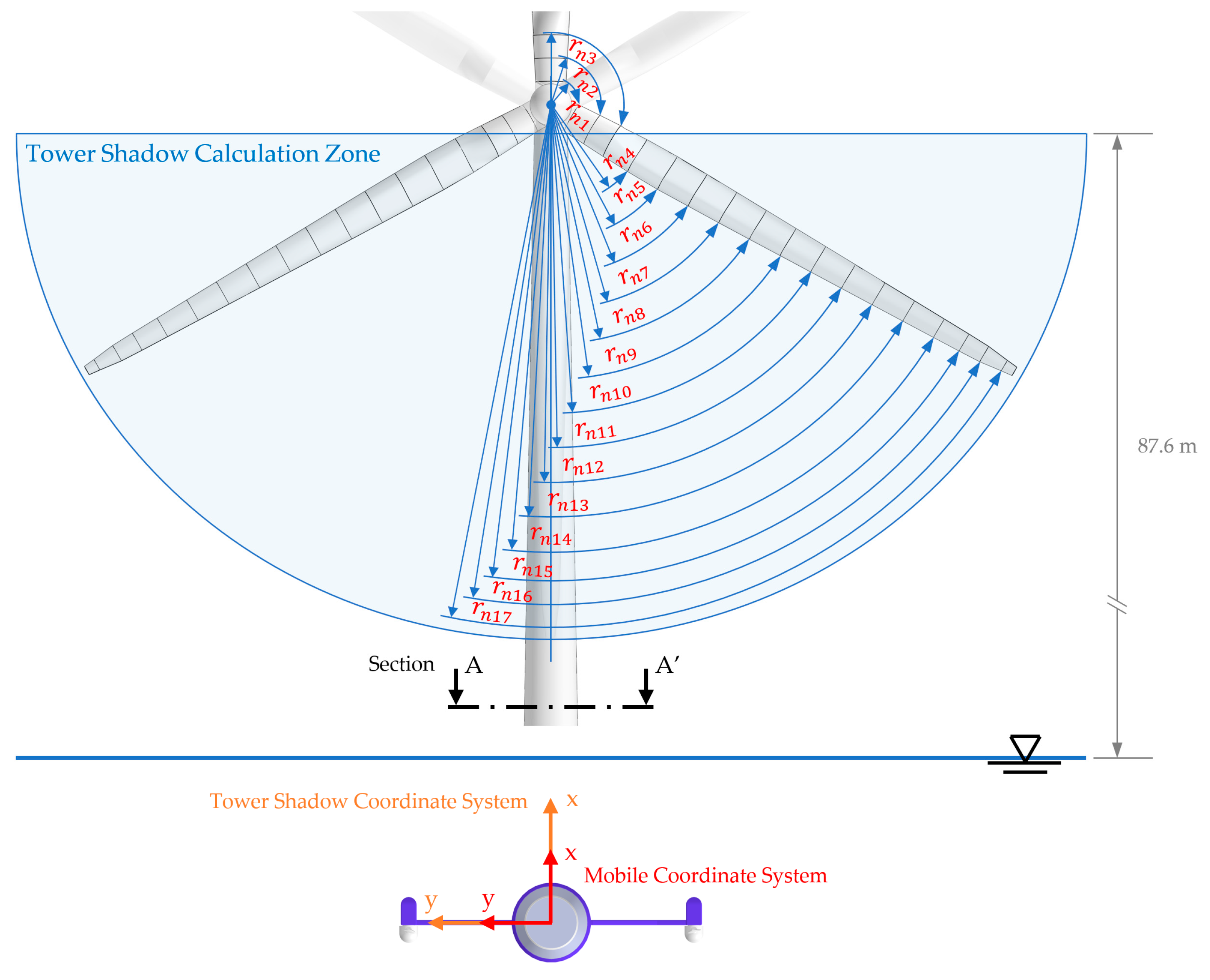
2.3.2. Blade Azimuth Position

This section describes the methodology used in FHYGSYS to calculate the blade azimuth position, that is, the angular position of the wind turbine rotor at each instant of time. As a previous step, the inertia tensor ( M I T   ( W T u r b i n e ) ) of the rotor—made up of the hub and the blades—of the wind turbine must be known. This inertia tensor is calculated at the center of mass ( C o M W T u r b i n e ) of the wind turbine rotor (see Figure 5). The calculation is simplified by calculating the inertia tensor with respect to a coordinate system with origins in C o M W T u r b i n e and whose axes are parallel to those of the mobile coordinate system (see Figure 12 of [37]). Next, the inertia tensor is rotated by the shaft tilt angle ( φ S h a f t   T i l t ) and then by the angle that represents the wind direction ( δ ), thus leaving the X axis of the coordinate system attached to the inertia tensor aligned in the direction of the axis of rotation of the wind turbine, represented by the unit vector u   s h a f t   ( B O D Y ) . This whole process is carried out based on the inertial data of the blade and hub of the wind turbine found in Appendix A in [36], following the explanation given in Section 2.3.2, also from [36]. Equation (50) shows the value of the inertia tensor ( M I T   ( W T u r b i n e ) ) calculated and positioned as indicated.
M I T   ( W T u r b i n e ) = [ I W T x x 0 0 0 I W T y y 0 0 0 I W T z z ] = [ 35196249 0 0 0 17930184 0 0 0 17930184 ]   kg · m 2
As we intended to find the angular position of the wind turbine rotor ( ψ r o t o r ( t ) ) and the inertia tensor ( M I T   ( W T u r b i n e ) ) was aligned—as indicated previously—with respect to a coordinate system whose X axis coincides with the direction of the axis of rotation of the wind turbine; to continue the calculations, the moment of inertia about this X axis ( I W T u r b i n e ) is extracted, ignoring the rest of the data of the inertia tensor. This is expressed in Equation (51).
I W T u r b i n e = I W T x x
As shown in Figure 5, the axis of rotation of the wind turbine is coupled with an electrical generator, which is responsible for converting the mechanical energy of the axis into electrical energy. This coupling causes an increase in the inertia of the axis of rotation due to the inertia ( I G E N ) of the electric generator (see Table 2). In Equation (52)—deduced from the explanation in [14]—this increase is expressed mathematically, yielding the total inertia of the rotor ( I r o t o r ), where g e a r R is the gearbox ratio found in Table 2. The coupling between the shaft and the electric generator in wind turbines has been widely discussed in the literature and works such as [45,46,47] have addressed this issue in more depth.
I r o t o r = I W T u r b i n e + I G E N · g e a r R 2
Similarly, the coupling between the axis of rotation of the wind turbine and the electric generator causes the existence of opposing torques in the shaft. These opposing torques are the low-speed shaft aerodynamic torque ( M a e r o s h a f t ( t ) ) (calculated in Equation (48)) and the low-speed shaft generator torque ( M G E N s h a f t ( t ) ). Equation (53) represents the opposition of these two torques on the shaft, yielding the low-speed shaft torque ( M r o t o r ( t ) ).
M r o t o r ( t ) = M a e r o s h a f t ( t ) M G E N s h a f t ( t )
The torque ( M G E N s h a f t ( t ) ) produced by the electric generator in the low-speed shaft (see Figure 5) is obtained through Equation (54), where M G E N ( t ) is the torque of the electric generator on the high-speed shaft (see Figure 5)—which depends on the control system (see Section 2.4.1)—with g e a r R being the gearbox ratio. Equations (53) and (54) can also be deduced from the explanation given in [14].
M G E N s h a f t ( t ) = M G E N ( t ) · g e a r R
From the results of Equations (52) and (53), Newton’s second law for rotation [48], expressed in Equation (55), can be applied, yielding the low-speed shaft angular acceleration ( α r o t o r ( t ) ) of the wind turbine.
α r o t o r ( t ) = M r o t o r ( t ) I r o t o r
Next, the laws of kinematics are applied, by integrating the low-speed shaft angular acceleration (through Equation (56)), the low-speed shaft angular speed ( ω r o t o r ( t ) ) of the turbine is obtained and, integrating this angular speed with Equation (57), the angular position ( ψ r o t o r ( t ) ) of the rotor can be found. These two integrals are solved in FHYGSYS by applying the method of Romberg’s algorithm [40], as explained in Appendix C in [36].
ω r o t o r ( t ) =   α r o t o r ( t ) · d t
ψ r o t o r ( t ) =   ω r o t o r ( t ) · d t
The result of the low-speed shaft angular speed ( ω r o t o r ( t ) ) calculated with Equation (56) is expressed in rad/s, but since it is usual to represent this angular speed in rpm ( Ω r o t o r ( t ) ), this calculation is included in Equation (58).
Ω r o t o r ( t ) = ω r o t o r ( t ) · 60 2 · π   r p m

2.3.3. Vector of Wind Turbine Forces

This calculation starts from the force vector ( F   b l a d e   j   ( B O D Y ) ( t ) ) exerted at the base of each blade ( p n 0 j   ( B O D Y ) ( t ) points), calculated using Equation (39). Equation (59) can be used to find the moment ( M   T h r u s t   j   ( B O D Y ) ( t ) ) produced by these force vectors at the origin of the mobile coordinate system.
M   T h r u s t   j   ( B O D Y ) ( t ) = p n 0 j   ( B O D Y ) ( t ) × F   b l a d e   j   ( B O D Y ) ( t ) = | i j k x n 0 j y n 0 j z n 0 j F x F y F z |
Next, the forces and moments that originated in each of the blades are added to obtain the total thrust ( F   T h r u s t   ( B O D Y ) ( t ) ) and moment ( M   T h r u s t   ( B O D Y ) ( t ) ) vectors produced by the wind turbine. This is achieved by means of Equations (60) and (61), respectively.
F   T h r u s t   ( B O D Y ) ( t ) = j = 1 B F   b l a d e   j   ( B O D Y ) ( t )
M   T h r u s t   ( B O D Y ) ( t ) = j = 1 B M   T h r u s t   j   ( B O D Y ) ( t )
The magnitude ( T T h r u s t ( t ) ) of the total thrust vector ( F   T h r u s t   ( B O D Y ) ( t ) ) calculated in Equation (60) is another important piece of information of the wind turbine model; for this reason, it is important to highlight it, as shown in Equation (62).
T T h r u s t ( t ) = | F   T h r u s t   ( B O D Y ) ( t ) |
At this point, the vector of wind turbine forces ( F k ( B O D Y )   W I N D   T U R B I N E ( t ) ) can be found by applying Equation (63), where k takes values from 1 to 6, representing the degrees of freedom (DOF) of the vector (1 = surge, 2 = sway, 3 = heave, 4 = roll, 5 = pitch, and 6 = yaw).
F k ( B O D Y )   W I N D   T U R B I N E ( t ) = [ F   T h r u s t ( B O D Y ) ( t ) M   T h r u s t ( B O D Y ) ( t ) + M   a e r o   ( B O D Y ) ( t ) M   r o t o r   ( B O D Y ) ( t ) ]
In this equation, the vectors F   T h r u s t   ( B O D Y ) ( t ) and M   T h r u s t   ( B O D Y ) ( t ) are those obtained in Equations (60) and (61), respectively, the vector M   a e r o   ( B O D Y ) ( t ) is the result of Equation (46) and the vector M   r o t o r   ( B O D Y ) ( t ) is calculated by applying Equation (64), where M r o t o r ( t ) is the result of Equation (53), and the unit vector u   s h a f t   ( B O D Y ) is the one obtained by Equation (49).
M   r o t o r   ( B O D Y ) ( t ) = M r o t o r ( t ) · u   s h a f t   ( B O D Y )
The vector of wind turbine forces ( F k ( B O D Y )   W I N D   T U R B I N E ( t ) ) calculated using Equation (63) is the main result of all the work presented in this article, since it represents the vector of forces and moments resulting from applying the BEM theory to the wind turbine, being the main milestone of everything described up to this moment in Section 2.
It could even be considered as the piece that completes the mathematical model discussed in [36,37], substituting the modeling of the turbines described in Section 2.8 in [37], which uses the One-Dimensional theory, by the one described in Section 2 of this work. In fact, this is what happens when FHYGSYS chooses to simulate the turbines using BEM theory.

2.3.4. Additional Magnitudes

The mathematical model presented in the previous subsections allows one to obtain the values of other important magnitudes that offer interesting information about the behavior of the turbine. These magnitudes are the different powers, the thrust and power coefficients, the axial and angular induction factors, the tip-speed ratio, and the average value of the angle of attack.
When applying BEM theory in FHYGSYS to model the turbines, three different powers can be obtained: electrical power ( P E L E ( t ) ), mechanical power ( P M E C ( t ) ), and aerodynamic power ( P A E R O ( t ) ). These powers can be calculated using Equations (65)–(67), where g e n E is the value of the electrical generator efficiency (see Table 2) and the rest of the values have been referred to on several occasions in the previous subsections.
P E L E ( t ) = ω r o t o r ( t ) · M G E N s h a f t ( t ) · g e n E
P M E C ( t ) = P E L E ( t ) g e n E
P A E R O ( t ) = ω r o t o r ( t ) · M a e r o s h a f t ( t )
As a previous step to the rest of the calculations, the area swept by the wind turbine blades ( A T u r b i n e ) is calculated using Equation (68), being the expression of the area of a circular crown. The radius of the turbine ( r T u r b i n e ) is obtained with Equation (20), and the radius of the hub ( r H u b ) is shown in Table 2.
A T u r b i n e = π · ( r T u r b i n e 2 r H u b 2 )
Another necessary value is the mean of the magnitude of the effective wind velocity vector ( V 0   ( A V ) ( t ) ) on each of the blades ( j ) applied to each of the blade elements ( i ). This value can be found by Equation (69), where V 0   i j ( t ) is obtained from Equation (12).
V 0   ( A V ) ( t ) = 1 B · j = 1 B ( 1 17 · i = 1 17 V 0   i j ( t ) )
With these data, the power ( C P ( t ) ) and thrust ( C T ( t ) ) coefficients are calculated from the values of the aerodynamic power ( P A E R O ( t ) ) obtained with Equation (67), and the thrust module ( T T h r u s t ( t ) ) found with Equation (62), taking as the value of the air density ρ A I R = 1.225   k g / m 3 . These coefficients can be calculated through Equations (70) and (71), respectively. Equation (70) was extracted from [2,3,4], while Equation (71) was extracted from [2,4].
C P ( t ) = P A E R O ( t ) 1 2 · ρ A I R · A T u r b i n e · V 0   ( A V ) 3 ( t )
C T ( t ) = T T h r u s t ( t ) 1 2 · ρ A I R · A T u r b i n e · V 0   ( A V ) 2 ( t )
The value of the tip-speed ratio ( T S R ( t ) ) can be obtained through Equation (72), extracted from [2,3,4].
T S R ( t ) = ω r o t o r ( t ) · r T u r b i n e V 0   ( A V ) ( t )
Finally, using Equations (73)–(75), the mean values of the angle of attack ( φ A t t a c k   ( A V ) ( t ) ), the axial induction factor ( a x i f ( A V ) ( t ) ), and the angular induction factor ( a n i f ( A V ) ( t ) ) can be calculated. In addition to presenting the average of these values, FHYGSYS can deliver the data individually to study the temporal evolution of these magnitudes in each blade element.
φ A t t a c k   ( A V ) ( t ) = 1 B · j = 1 B ( 1 17 · i = 1 17 φ A t t a c k   i j ( t ) )
a x i f ( A V ) ( t ) = 1 B · j = 1 B ( 1 17 · i = 1 17 a x i f i j ( t ) )
a n i f ( A V ) ( t ) = 1 B · j = 1 B ( 1 17 · i = 1 17 a n i f i j ( t ) )

2.4. Wind Turbine Control System

As indicated in Section 2.2.1 and Section 2.3.2, there are two magnitudes whose values depend on the control system of the floating hybrid system, in other words, the control system establishes the appropriate value of these magnitudes so that the wind turbine works in the desired way in each instant of time. These magnitudes are the torque ( M G E N ( t ) ) of the electric generator on the high-speed shaft and the collective blade pitch angle ( φ P i t c h ( t ) ).
The control system of the floating hybrid system consists of two closed-loop PID controllers. One controls the generator torque ( M G E N ( t ) ) when the wind speed ( V W R E F ) is between 3 m/s and 11.4 m/s, and the other controls the collective blade pitch angle ( φ P i t c h ( t ) ) when the wind speed ( V W R E F ) is between 11.4 m/s and 25 m/s. These speed ranges correspond to those established in the design of the “OC3-Hywind” wind turbine described in [14,49]. As the floating hybrid system clearly has a nonlinear behavior, a gain schedule was implemented for the operation of each of the PID controllers.
The modeling of the control system works independently of the mathematical model of the floating hybrid system, and interacts with the turbine modeling described in previous sections. Despite this, the control system was also implemented mathematically as well as the actuators of each controller. Figure 9 shows the block diagram of the control system interacting with the wind turbine (plant) of the floating hybrid system, where the separation between these mathematical models can be observed.
The only connection between the two mathematical models is produced (resembling the operation of a real system) through three magnitudes: the generator torque ( M G E N ( t ) ) and the collective blade pitch angle ( φ P i t c h ( t ) ) as inputs to the plant, and the high-speed shaft angular speed ( ω G E N ( t ) ) as the output of it.
Figure 9 clearly shows how the two controllers work: the torque controller modifies the low-speed shaft generator torque ( M G E N s h a f t ( t ) ) to obtain the desired wind turbine speed ( ω r o t o r ( t ) ), while the pitch controller modifies, indirectly, the low-speed shaft aerodynamic torque ( M a e r o s h a f t ( t ) ) to achieve the same goal, the desired wind turbine speed.
From the analysis of the block diagram in Figure 9, some relationships can be deduced. Equation (76) allows one to obtain the difference ( ω e r r o r ( t ) ) between the angular speed to be reached ( ω S P ), which establishes the set point, and the high-speed shaft angular speed ( ω G E N ( t ) ), which is the angular speed of the electrical generator at a given instant of time.
ω e r r o r ( t ) = ω S P ω G E N ( t )
Equation (77) establishes the relationship between the low-speed shaft angular speed ( ω r o t o r ( t ) ) and the high-speed shaft angular speed ( ω G E N ( t ) ), where g e a r R is the gearbox ratio.
ω G E N ( t ) = ω r o t o r ( t ) · g e a r R
Figure 9 also illustrates Equation (53), which relates the low-speed shaft aerodynamic torque ( M a e r o s h a f t ( t ) ) with the low-speed shaft generator torque ( M G E N s h a f t ( t ) ), yielding the low-speed shaft torque ( M r o t o r ( t ) ). Likewise, Equation (54) is also derived, which relates the low-speed shaft generator torque ( M G E N s h a f t ( t ) ) with the torque of the electric generator on the high-speed shaft ( M G E N ( t ) ) through the gearbox ratio.
Because FHYGSYS is a time-domain simulation tool, the mathematical expression used for the modeling of the controllers is the one described in [50] for the time-domain modeling of PID controllers, as shown in Equation (78), in which K p , T i , and T d are the parameters that define the behavior of the PID controller (proportional gain, integration time, and derivative time, respectively), e(t) is the error value (the input value to the controller), and u ( t ) is the output value of the PID controller.
u ( t ) = K p · ( e ( t ) + 1 T i ·   e ( t ) · d t + T d · d d t · e ( t ) )
Equation (78) is the general expression of a PID controller, but in the controllers implemented in the control system of the floating hybrid system, the derivative action has not been included because with the proportional and integral actions, it is possible to reach the conditions of operation of the wind turbine indicated in [14].
The integral that appears in Equation (78) is solved in FHYGSYS by applying the method of Romberg’s algorithm [40].

2.4.1. Generator Torque Controller

As indicated in the previous section, the generator torque controller is in operation for wind speeds ( V W R E F ) between 3 m/s and 11.4 m/s. Above these wind speeds, the generator torque ( M G E N ( t ) ) is equal to the rated generator torque ( Q G E N r a t e d ), whose value can be found in Table 2, in the same way as in [14].
On the other hand, as explained in [14], the PID torque controller starts operating when the high-speed shaft angular speed ( ω G E N ( t ) ) exceeds the minimum generator speed to connect the torque controller ( ω G E N m i n ), which appears in Table 2. Until that instant of time, the low-speed shaft aerodynamic torque ( M a e r o s h a f t ( t ) ) accelerates the wind turbine [14], while the generator torque ( M G E N ( t ) ) is equal to zero.
The main objective of FHYGSYS is to provide a simulation tool for a floating hybrid system like the one shown in Figure 1, which allows for experimentation with different control strategies. For this reason, in the design process of this first control system at FHYGSYS, it was decided to control the generator torque directly with a gain scheduled PID controller, unlike the strategy described in [14], in which different torque control guidelines were established depending on the wind speed ( V W R E F ).
However, the gain scheduled PID controller was based on the wind turbine speed ( Ω S P ( t ) ) as a function of each wind speed ( V W R E F ) described in [14,49]. The wind turbine speed ( Ω S P ( t ) ) is the set point speed expressed in rpm in the low-speed shaft. This is related to the set point in the high-speed shaft angular speed ( ω S P ), which appears in Equation (76) through the gearbox ratio ( g e a r R ), expressing the result in rad/s.
Table 4 shows the gain scheduled established in FHYGSYS for the operation of the torque PID controller. The values of wind turbine speed ( Ω S P ( t ) ), proportional gain ( K p G E N ), and integration time ( T i G E N ) were established as a function of wind speed ( V W R E F ), performing linear interpolation for intermediate values of this.
Figure 10 shows the behavior of the wind turbine speed ( Ω r o t o r ( t ) ) obtained in Equation (58)–with and without the torque control system in operation and compares the results with those obtained by FASTv8 under the same conditions. It shows what would happen when the low-speed shaft generator torque ( M G E N s h a f t ( t ) ), for whatever reason, takes the zero value; in this situation, the low-speed shaft aerodynamic torque ( M a e r o s h a f t ( t ) ) produces an uncontrolled increase in the wind turbine speed. This justifies the importance of the torque control system.
Equation (79) yields the control action ( u M G E N ( t ) ) of the torque controller (being a particularization of Equation (78)), where K p G E N and T i G E N are the proportional gain and integration time of the gain scheduled PID controller (see Table 4) and ω e r r o r ( t ) is the error angular speed obtained with Equation (76).
u M G E N ( t ) = K p G E N · ( ω e r r o r ( t ) + 1 T i G E N ·   ω e r r o r ( t ) · d t )
In order to avoid the windup effect in the controller, the value of the integral of the error angular speed ( ω e r r o r ( t ) ) of the controller is kept at zero until the generator reaches the minimum generator speed ( ω G E N m i n ) to connect the torque controller (see Table 2).
In a similar way as to how a PID controller is implemented in industrial devices—as in a PLC (Programmable Logic Controller)—the output of the generator torque PID controller is scaled, as shown in Equation (80).
{     u M G E N ( t ) > 1     u M G E N ( t ) = 1   u M G E N ( t ) < 1     u M G E N ( t ) = 1
To complete the description of the elements that make up the closed-loop torque controller, it remains to describe the equations that define the behavior of the generator torque actuator (see Figure 9). For this, a linearized behavior was considered based on the data included in Table 5.
From the data in Table 5, the equation of a straight line can be obtained, showing the result in Equation (81).
M G E N ( t ) = Q G E N r a t e d · ( 1 u M G E N ( t ) )
The modeling of the torque controller actuator is completed by establishing its operating limits. On the one hand, Equation (82) establishes the maximum and minimum values that the generator torque (MGEN(t)) can take.
{     M G E N ( t ) > Q G E N r a t e d     M G E N ( t ) = Q G E N r a t e d   M G E N ( t ) < 0     M G E N ( t ) = 0
On the other hand, through Equation (83), the maximum values of the rise or fall of the generator torque can be established. Both the values of Q G E N r a t e d and Δ Q G E N r a t e d are shown in Table 2.
| d d t M G E N ( t ) | > Δ Q G E N r a t e   {     d d t M G E N ( t ) > 0     d d t M G E N ( t ) = Δ Q G E N r a t e d d t M G E N ( t ) < 0     d d t M G E N ( t ) = Δ Q G E N r a t e

2.4.2. Collective Blade Pitch Angle Controller

As indicated at the beginning of Section 2.4, the collective blade pitch angle controller is in operation for wind speeds ( V W R E F ) between 11.4 m/s and 25 m/s. Below these wind speeds, the collective blade pitch angle ( φ P i t c h ( t ) ) is zero, in the same way as in [14].
As explained in the previous case, the gain scheduled PID controller is based on the wind turbine speed ( Ω S P ( t ) ) (set point speed) as a function of each wind speed ( V W R E F ) described in [14,49].
Table 6 shows the gain scheduled established in FHYGSYS for the operation of the collective blade pitch angle PID controller. The values of wind turbine speed ( Ω S P ( t ) ), proportional gain ( K p P i t c h ), and integration time ( T i P i t c h ) were established as a function of wind speed ( V W R E F ), also performing linear interpolation for intermediate values of this.
From the analysis of Equation (76), it can be observed that if the speed of the high-speed shaft angular speed ( ω G E N ( t ) ) is greater than the set point speed ( ω S P ), the error angular speed ( ω e r r o r ( t ) ) is negative. This implies that the rated rotor speed ( Ω r a t e d ( t ) , see Table 2) has been exceeded. This is the situation in which the pitch controller in FHYGSYS should start. In order to adjust the pitch angle PID controller so that it can be put into operation before this situation occurs, the trigger offset factor ( F T r i g g ( % ) ) was introduced, which appears in Table 6. Equation (84) scales the trigger offset factor ( F T r i g g ( % ) ) so that it can be used in conjunction with the control action ( u P i t c h ( t ) ), yielding the pitch controller trigger offset factor ( F T r i g g ).
F T r i g g = F T r i g g ( % ) 100
Figure 11 shows the behavior of the wind turbine speed ( Ω r o t o r ( t ) ) obtained in Equation (58) in three situations.
The first case is in normal conditions, when the two controllers are active, one delivering the maximum torque of the generator ( M G E N ( t ) = Q G E N r a t e d ) and the other applying the corresponding pitch angle (red line). This situation was compared with the results obtained by FASTv8 (blue line) under the same conditions.
The second case shows what happens if the pitch controller is disconnected and only the torque controller works (green line). In this case, the wind turbine speed ( Ω r o t o r ( t ) ) exceeds the rated rotor speed ( Ω r a t e d ( t ) ), exceeding the operating limits and producing the destruction of the turbine.
In the third case, the uncontrolled increase in the wind turbine speed ( Ω r o t o r ( t ) ) produced by the absence of control is observed (orange line), which would produce catastrophic consequences.
This justifies the importance of the existence of a floating hybrid system control system for proper operation.
Equation (85) shows the equation of the collective blade pitch angle PID controller derived, as in the torque controller, from Equation (78). Equation (85) yields the control action ( u P i t c h ( t ) ) from the error angular speed ( ω e r r o r ( t ) ), the proportional gain ( K p P i t c h ), and the integration time ( T i P i t c h ).
u P i t c h ( t ) = K p P i t c h · ( ω e r r o r ( t ) + 1 T i P i t c h ·   ω e r r o r ( t ) · d t )
As in the previous case, the output of the controller ( u P i t c h ( t ) ) is scaled as indicated in Equation (86).
{     u P i t c h ( t ) > 1     u P i t c h ( t ) = 1   u P i t c h ( t ) < 1     u P i t c h ( t ) = 1
The last step is to present the equations that define the behavior of the blade pitch angle actuator (see Figure 9). In a similar way to the previous case, a linearized behavior based on the data in Table 7 was considered.
From the data in Table 7, the equation of a straight line can be obtained, showing the result in Equation (87).
φ P i t c h ( t ) = φ P i t c h m a x 1 + F T r i g g · ( F T r i g g u P i t c h ( t ) )
In this case, the modeling of the blade pitch angle actuator is also completed by establishing its operating limits, being equivalent to the previous case. On the one hand, Equation (88) establishes the maximum and minimum values that the pitch angle (φPitch(t)) can take.
{     φ P i t c h ( t ) > φ P i t c h m a x     φ P i t c h ( t ) = φ P i t c h m a x   φ P i t c h ( t ) < 0     φ P i t c h ( t ) = 0
On the other hand, through Equation (89), the maximum values of the rise or fall of the pitch angle are established. Both the values of φ P i t c h m a x and Δ φ P i t c h r a t e are shown in Table 2.
| d d t φ P i t c h ( t ) | > Δ φ P i t c h r a t e   {     d d t φ P i t c h ( t ) > 0     d d t φ P i t c h ( t ) = Δ φ P i t c h r a t e d d t φ P i t c h ( t ) < 0     d d t φ P i t c h ( t ) = Δ φ P i t c h r a t e
An important issue to highlight regarding the FHYGSYS control system described in this section is that when the pitch angle ( φ P i t c h ( t ) ) takes values greater than zero, this implies, as indicated before, that the rated rotor speed ( Ω r a t e d ( t ) ) has been exceeded; the torque controller forces the generator torque ( M G E N ( t ) ) to be equal to the rated generator torque ( Q G E N r a t e d ).

2.5. Application of BEM Modeling to Marine Current Turbines

This section explains the differences and similarities between the application of the wind turbine modeling methodology, as described in previous sections, with respect to those of MCTs.
The first step is to obtain the magnitude of the effective fluid velocity vector ( V 0 ( t ) ) with Equation (12), which, in this case, is based on the explanation of Section 2.3.2 in [37] for the sub-surface current modeling. This causes Equation (9) from [37] to be used instead of Equation (4), and the flow direction is ε , the sub-surface current direction, instead of δ in Equations (5) and (49).
A similar correction was also made to model the tower shadow effect, which in this case was called the support shadow effect. This correction is based on the data in Table 8.
Figure 12 illustrates the modeling used to correct the support shadow effect by applying the data from Table 8.
In the case of the wind turbine, the tower shadow coordinate system matches the mobile coordinate system (see Figure 4), so the components of the p n i   ( B O D Y ) ( t ) points in Equation (8) are used directly. By analyzing Figure 12, it can be verified that this did not occur in this case, so each p n i   ( B O D Y ) ( t ) point must be expressed in the corresponding turbine coordinate system using Equation (90).
[ x p n i   ( M C T ) y p n i   ( M C T ) z p n i   ( M C T ) ] = p n i   ( M C T ) ( t ) = [ cos ( ε ) sin ( ε ) 0 sin ( ε ) cos ( ε ) 0 0 0 1 ] · ( p n i   ( B O D Y ) ( t ) p o C M C T   ( B O D Y ) )
It is not necessary to use a transformation matrix in this equation for the change between systems since the axes of the mobile coordinate system and the turbine coordinate systems are parallel. In Equation (90), the center of the clockwise turbine has been used, but the equation is equivalent using the center of the counterclockwise turbine. Both points can be found in Table 9, while the value of the p n i   ( B O D Y ) ( t ) points can be found in Appendix A.
Similar to the case of the wind turbine, the support shadow effect calculation is applied only when the Y component of the p n i   ( M C T ) ( t ) points is less than zero in the case of the clockwise turbine, or greater than zero in the case of the counterclockwise turbine.
As can be seen in Figure 12, each support is made up of three tubes, so the equation (extracted from [4]) that models the support shadow effect must be applied three times, adapting the formula to the position of the support of MCTs. This is achieved by Equation (91), where the factor F c e n t e r s h a d o w represents the shadow effect of the central tube.
F c e n t e r s h a d o w = 1 ( D t u b e 2 ) 2 · ( x p n i   ( M C T ) 2 z p n i   ( M C T ) 2 ) ( x p n i   ( M C T ) 2 + z p n i   ( M C T ) 2 ) 2
The calculation of the shadow effect of the upper and lower tube is carried out only when the Y component of p n i   ( M C T ) ( t ) exceeds the length l h u b j u n c t i o n within each support shadow calculation zone (see Figure 12). In this situation, a value ( Δ z p n i   ( M C T ) ) is calculated through Equation (92) that corrects the Z component of the p n i   ( M C T ) ( t ) point by applying linear interpolation from the data in Table 8.
Δ z p n i   ( M C T ) = l t u b e m a x · l h u b j u n c t i o n | y p n i   ( M C T ) | l h u b j u n c t i o n l h u b p l a t f o r m
Increasing and decreasing the Z component of the p n i   ( M C T ) ( t ) point with the result of Equation (92), Equation (91) is applied with the new corrected values of the Z component of the p n i   ( M C T ) ( t ) point, yielding the factors F u p s h a d o w and F d o w n s h a d o w .
The modeling of the support shadow effect ends by applying Equation (93), which provides a result equivalent to that obtained with Equation (8).
v   S S C U R   s u p p o r t s h a d o w     ( B O D Y ) ( h ) = v   S S C U R   ( B O D Y ) ( h ) · F c e n t e r s h a d o w · F u p s h a d o w · F d o w n s h a d o w
From this point, the rest of the steps until calculating the magnitude of the effective fluid velocity vector ( V 0 ( t ) ) with Equation (12) are equivalent.
For the calculations in Section 2.2, Section 2.3 and Section 2.4, it is also necessary to define the properties of the MCTs, which are shown in Table 10.
In the case of MCTs, it is also necessary to know the aerodynamic characteristics of airfoils, or rather, the hydrodynamic characteristics of hydrofoils. As indicated in [38], the behavior of hydrofoils in water is analogous to the behavior of airfoils in air, the main difference between them being fluid density. This allows for the use of airfoil data for the modeling of MCTs without any additional correction.
The modeling of the MCTs used in the floating hybrid system was based on the design presented in [34,35], where a single hydrofoil (airfoil) is used for the design of the blades. This hydrofoil is the NACA 63-424.
From Equation (17), the angle of attack ( φ A t t a c k ( t ) ) can be obtained, and as in the case of the wind turbine, with these data expressed in degrees, the airfoil-data (hydrofoil-data) tables corresponding to each blade element were consulted to obtain the values of the lift coefficient ( C L ( t ) ), drag coefficient ( C D ( t ) ), and pitching-moment coefficient ( C M ( t ) ).
Table 11 shows the hydrodynamic properties of marine current turbine blades.
The data shown in Table 11 for each blade differential ( d p n i )—blade element—and their centers ( p n i ) were obtained by dividing the blade length ( L B l a d e ) of the MCTs (see Table 10) into 17 portions. The twist angle ( φ T w i s t ) and chord length ( L C h o r d ) data were obtained by performing linear interpolation from the data in Table 4 in [34], in which the blade was divided into 74 blade elements. This adaptation was carried out by equivalence with the data presented in [14] of the wind turbine blades, and used in this work after verifying that no significant differences were observed between the marine current turbine simulation results obtained with 17 and 74 blade elements. However, the computational cost was considerably reduced.
The hydrofoil-data tables of the NACA 63-424 and cylinder 3, which appear in Table 11, can be found in Appendix D in [51] and were used without any additional correction.
Figure 13 shows the unit vectors u   B j   t h r u s t , u   s h a f t , and u   M j   p i t c h i n g that replace those shown in Figure 5 and were used on several occasions in the turbine modeling calculations.
The values of the vectors u   B j   t h r u s t and u   M j   p i t c h i n g can be found in Appendix A. As seen in Figure 13, each of the two MCTs rotated in opposite directions, which implies that when dealing with the counterclockwise turbine, the sign of the unit vector u   s h a f t calculated with Equation (49) is changed. This practice is usually used in boats with two propellers to compensate for the moments produced by each of them. This technique is even used in tandem-rotor helicopters for the same reason.
This feature can be used as a control strategy for yaw compensation, turning each MCT at a different speed.
The application of the rest of the equations of the model described in Section 2.2 and Section 2.3, was carried out in an equivalent way to the two MCTs, although they rotated in different directions. It is only necessary to use the unit vectors (shown in Figure 13) appropriate to the corresponding turbine.
The only exception to consider is that the MCTs are always completely submerged in the sea, so, unlike the wind turbine, the density of the fluid interacting with them is that of seawater. Therefore, the density used in Equations (33), (34), (70) and (71) was ρ S E A   W A T E R = 1025   kg / m 3 .
This also implies that in the calculation of the inertia tensor in Equations (50)–(52), the inertia tensor caused by the added mass of the MCTs must be taken into account. Therefore, Equation (52) can be redefined as indicated in Equation (94).
I r o t o r = I M C T u r b i n e + I M C T u r b i n e   ( S U M ) + I G E N · g e a r R 2
Equation (95) shows the inertia tensor of the clockwise turbine, while Equation (96) shows the inertia tensor of the added mass of the same turbine. These results were obtained from the inertial data in Appendix A in [36].
M I T   ( M C T T u r b i n e ) = [ I M C T x x 0 0 0 I M C T y y 0 0 0 I M C T z z ] = [ 169177 0 0 0 169584 2884 0 2884 11241 ]   kg · m 2
M I T   ( M C T T u r b i n e   ( S U M ) ) = [ I M C T x x   ( S U M ) 0 0 0 I M C T y y   ( S U M ) 0 0 0 I M C T z z   ( S U M ) ] = [ 107768 0 0 0 108304 1873 0 1873 5413 ]   kg · m 2
The difference between these inertia tensors and those of the counterclockwise turbine is in the sign of the products of inertia of the inertia tensor. The data needed to solve Equation (94) are, as in the case of the wind turbine, the moments of inertia with respect to the X axis of the two inertia tensors represented in Equations (95) and (96). Therefore, the inertia tensors of the counterclockwise turbine are omitted.
In Equations (97) and (98), the moments of inertia necessary to solve Equation (94) are represented mathematically.
I M C T u r b i n e = I M C T x x
I M C T u r b i n e   ( S U M ) = I M C T x x   ( S U M )

2.6. Marine Current Turbines Control System

The control system of the MCTs is designed in FHYGSYS in the same way as for the wind turbine. It is also based on two gain scheduled PID controllers: one to control the torque of the generators ( M G E N ( t ) ), and another to control the collective pitch angle of the blades ( φ P i t c h ( t ) ).
Each of the controllers of the two MCTs act individually. This means that when the three turbines of the floating hybrid system are in operation, there are three PID controllers governing each turbine independently, but not in a coordinated way.
The gain scheduled of both the torque and collective pitch angle controllers of the two MCTs are the same.
Table 12 shows the gain scheduled for the torque controller.
Completing the data from the control system of the MCTs, Table 13 shows the gain scheduled for the collective pitch angle controller.

3. Results

In order to present the work carried out as completely as possible, we performed two simulations in which a fluid velocity sweep is made from the lowest to the highest value at which the turbines can operate. These maximum and minimum values of fluid velocity are those shown in the gain schedules in Table 4, Table 6, Table 12 and Table 13. In each test, the most relevant magnitudes are represented, whose calculations were described throughout Section 2.
In this section, the titles of the figures that include graphs of the different magnitudes as well as the nomenclature that appears in them are the same used by FASTv8.

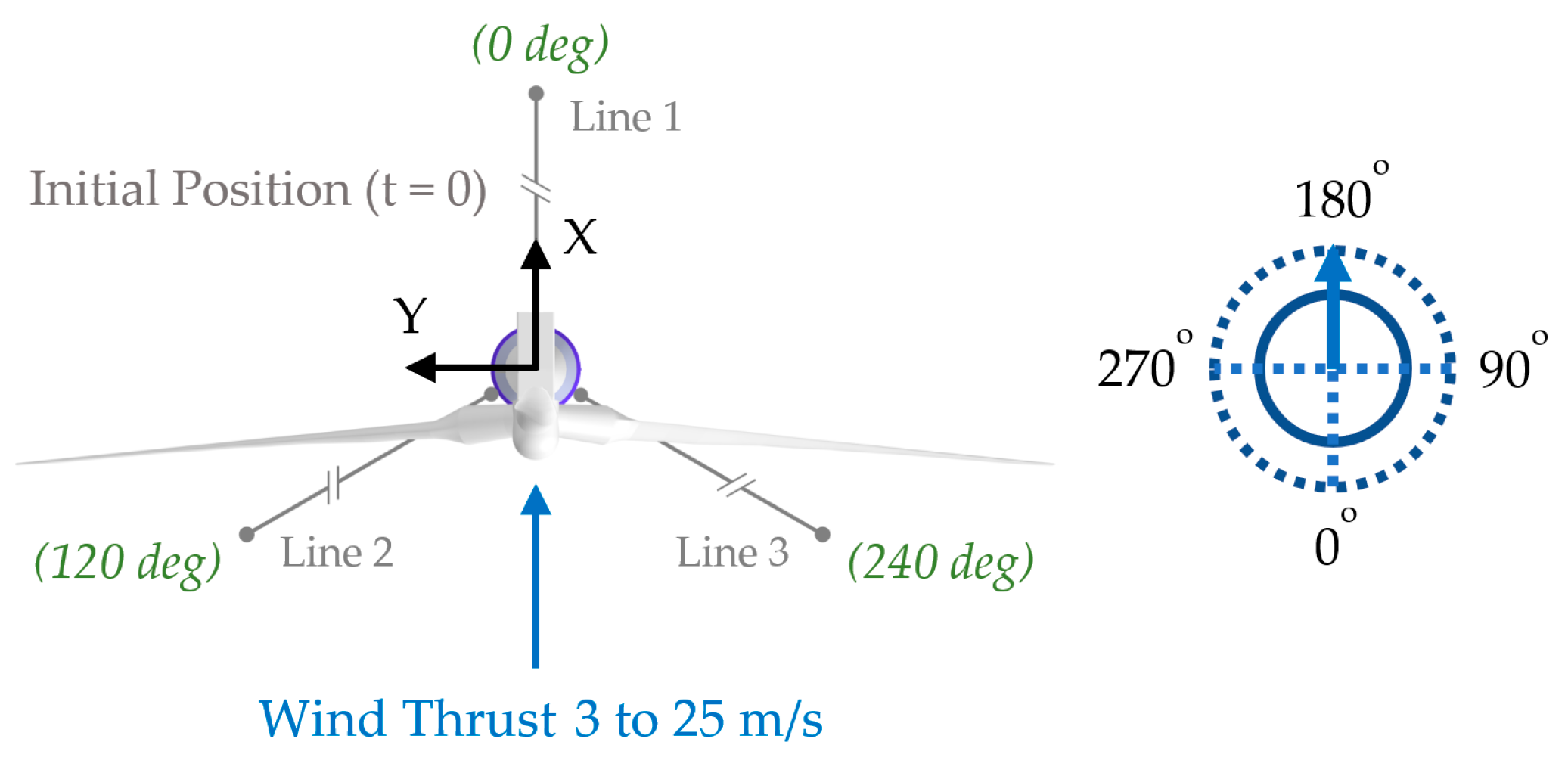
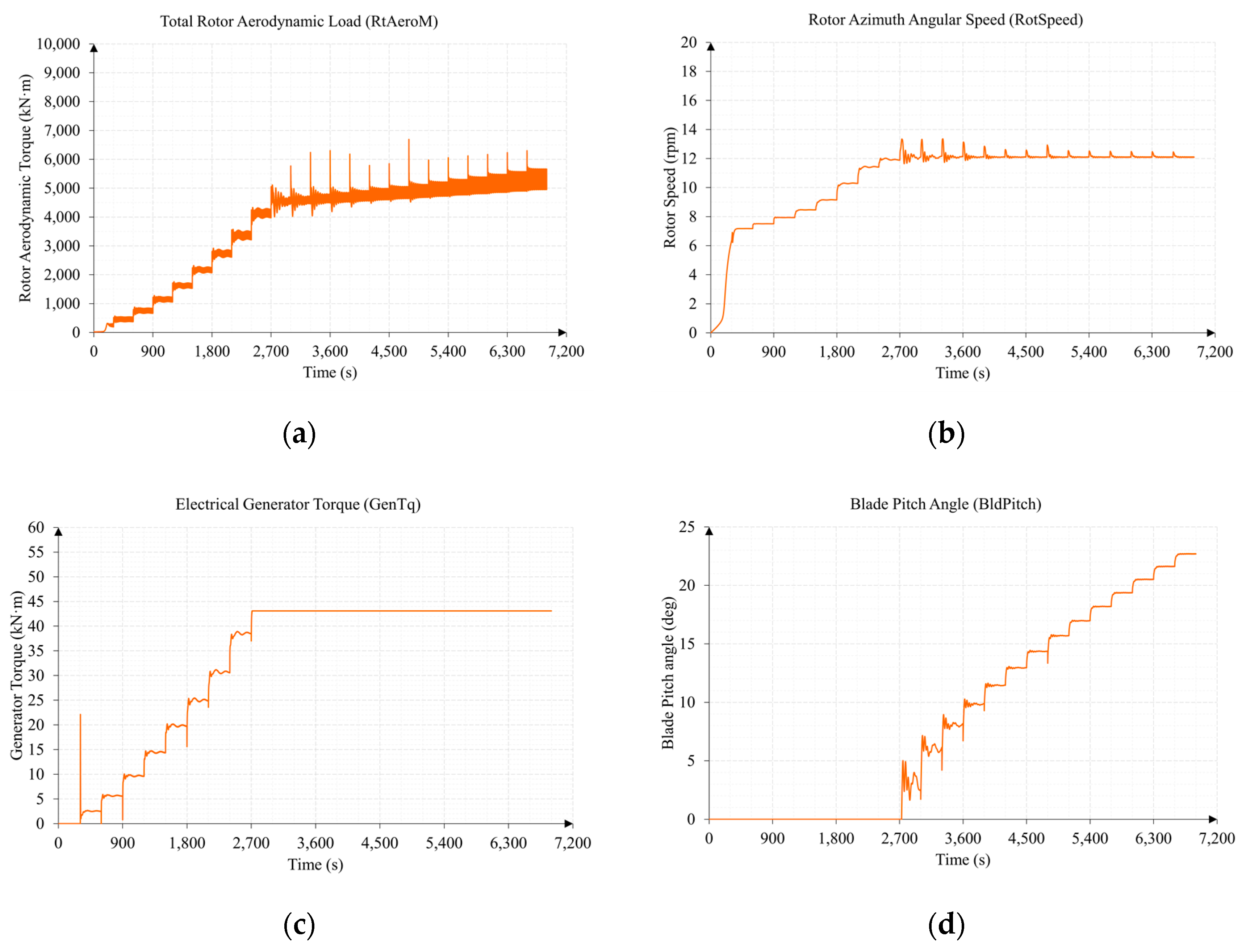
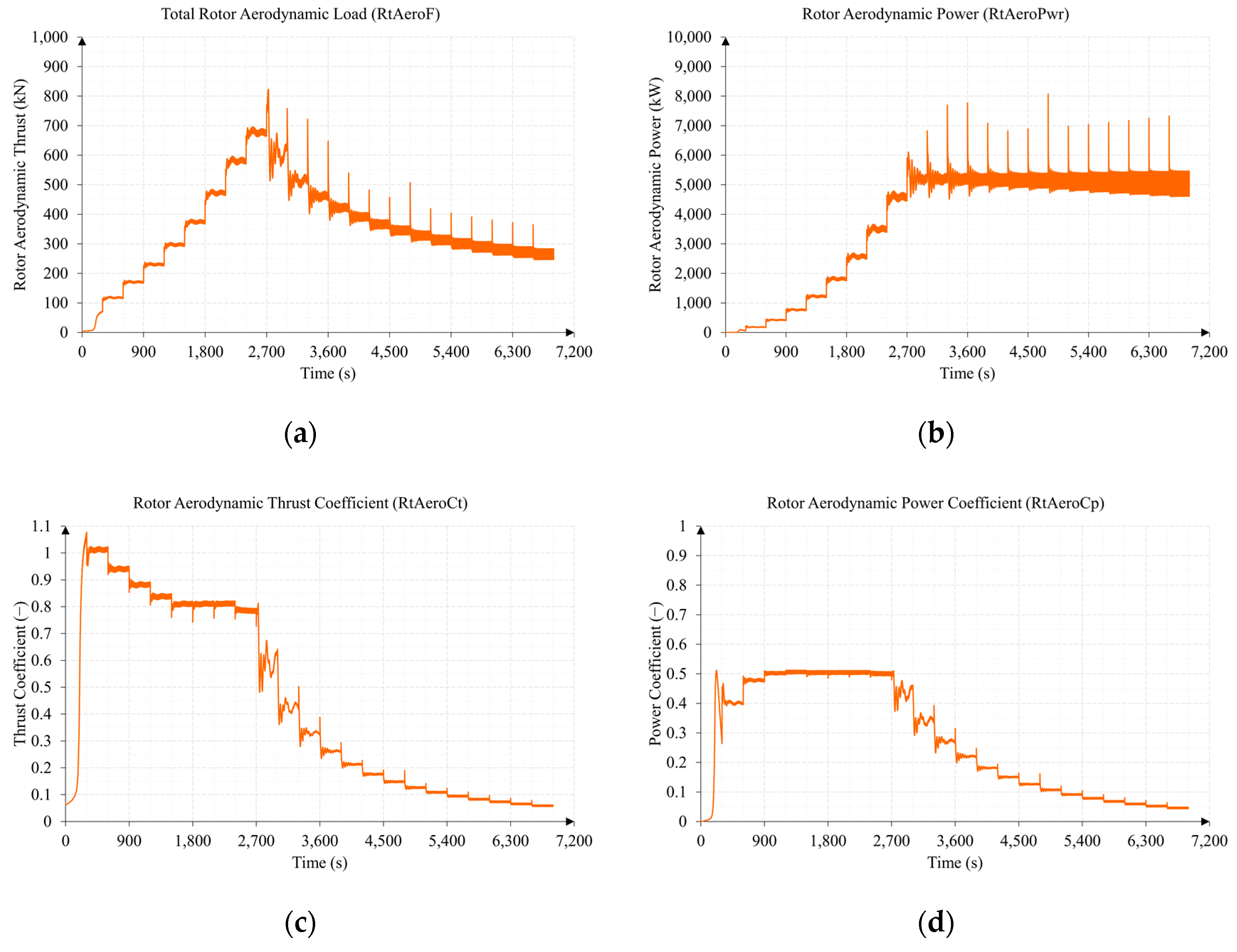
3.1. Test 1. Wind Speed Sweep from 3 to 25 m/s

Figure 14 shows the configuration of Test 1, in which a sweep of wind speeds was made from 3 to 25 m/s, with a direction of zero degrees, a sub-surface current speed of 0 m/s, and without the presence of waves.
As shown in Figure 14, in Test 1, the “OC3-Hywind” version without MCTs implemented in FHYGSYS was used. As can be seen in Figure 15a, the sweep of wind speeds was carried out increasing the wind speed ( V W R E F ) by 1 m/s every 300 s. Tests were performed for all of these speeds and a code-to-code comparison was made with simulations carried out with FASTv8 under the same conditions, obtaining satisfactory results. Two examples of these validation simulations are shown in Appendix B.
Figure 15b shows the graph of the electrical power generated ( P E L E ( t ) )—the main magnitude of the installation—in which it reaches the maximum power from a wind speed of 12 m/s. Figure 16 shows the graphs of the six degrees of freedom of the floating hybrid system.
An increase in surge and pitch was observed as the wind speed increased and just when the power generated reached its maximum; as the wind speed continued to increase, these degrees of freedom decreased. However, in sway and roll, an increase was observed whenever the wind speed increased, with the variations in heave and yaw of little relevance. These results corresponded to those expected, considering the angle of incidence of the wind on the floating hybrid system (see Figure 14) and that the wind turbine rotated clockwise.
Figure 17 shows the behavior of the two input magnitudes that control the wind turbine (see Figure 9): electrical generator torque ( M G E N ( t ) ) and collective blade pitch angle ( φ P i t c h ( t ) ). It was also observed how these affected the rotor aerodynamic torque ( Q a e r o ( t ) ) and the rotor speed ( Ω r o t o r ( t ) ) of the turbine.
The electrical generator torque opposes the rotor aerodynamic torque to achieve the desired rotor speeds until the rated generator torque ( Q G E N r a t e d ) is reached (see Table 2). At this wind speed, which is approximately 12 m/s, the rated rotor speed ( Ω r a t e d ) is reached (see Table 2). From that wind speed, the collective blade pitch angle is responsible for slowing down the increase in rotor aerodynamic torque and keeping the rated rotor speed as stable as possible.
Figure 18 shows the relationship between the rotor thrust ( T T h r u s t ( t ) ) exerted by the wind turbine and the rotor aerodynamic power ( P A E R O ( t ) ) present in the low-speed shaft with their respective coefficients: the thrust coefficient ( C T ( t ) ) and the power coefficient ( C P ( t ) ) respectively. Figure 18a shows how the rotor thrust increases as the wind speed increases until the rated generator torque is reached. From this wind speed, the collective blade pitch angle behaves like an aerodynamic brake, decreasing the rotor thrust exerted by the wind turbine as this angle increases.
The rotor aerodynamic power behaves in a similar way to the electrical generator power (see Figure 15b), settling around the maximum power of the wind turbine once the rated rotor speed is reached. Figure 18c shows how the C T ( t ) stabilizes around 0.8 for intermediate wind speeds and how it decreases drastically as the wind speed increases once the rated rotor speed is reached. The C P ( t ) behaves in a similar way to the C T ( t ) , showing a high efficiency—considering the Betz limit [2,3,4]—for intermediate wind speeds, decreasing as the wind speed increases once the wind turbine reaches the situation of maximum wind energy absorption.
Figure 19 shows the tip-speed ratio ( T S R ( t ) ) and the 27 C P / 16 T S R curve.
It is common to use graphical representations of C P T S R to evaluate the efficiency of the wind turbine [2,3,4], in which the maximum value that can be reached is below the Betz limit. This representation can also be made by normalizing the C P ( t ) value with the Betz limit [2], obtaining 27 C P / 16 T S R graphs like the one shown in Figure 19b, which shows the evolution of C P ( t ) between 0 and 1 as a function of the T S R ( t ) . Analyzing Figure 19b, it can be observed that the maximum efficiency of the wind turbine is around 0.85, obtained for a T S R ( t ) between 8 and 9. Comparing these observations with Figure 18d and Figure 19a, it was verified that the maximum efficiency of the wind turbine occurred for intermediate values of wind speed, in which a higher C P ( t ) was obtained.
Figure 20 shows the control actions of the two PID controllers, with which their behavior can be analyzed.
Comparing Figure 17c and Figure 20a, it was observed that the control action ( u M G E N ( t ) ) of the torque controller manages the value of the generator torque ( M G E N ( t ) ) when it is positive, since when it reaches negative values the generator torque takes the value of the rated generator torque ( Q G E N r a t e d ). This behavior is consistent with the modeling of the generator torque actuator shown in Table 5.
As indicated in Section 2.4.2, a design criterion of the control system is that when the collective blade pitch angle is greater than zero, the torque controller forces the generator torque to be equal to the rated generator torque. For this reason, around 2700 s, although the torque control action still delivers positive values, since the pitch angle already takes positive values (see Figure 17d), the value of the generator torque is equal to the rated generator torque.
Similarly, the control action ( u P i t c h ( t ) ) of the collective blade pitch controller (see Figure 20b) manages the value of the pitch angle when it is negative. However, due to the value of the trigger offset factor ( F T r i g g ( % ) ), it is possible for the pitch controller to start working before the rated rotor speed is exceeded, obtaining positive pitch angle values in this situation. This behavior is also consistent with the modeling of the collective blade pitch angle actuator shown in Table 7. Figure 20c,d shows the behavior, by way of illustration, of the integral control actions of the controllers; these are part of the control actions, as can be deduced from Equations (79) and (85).
The scaling of Figure 16, Figure 17b,d, Figure 18a,c,d, Figure 19 and Figure 20 was conducted in the same manner as that of the equivalent figures of Test 2, in order to more easily compare the results between the two tests.

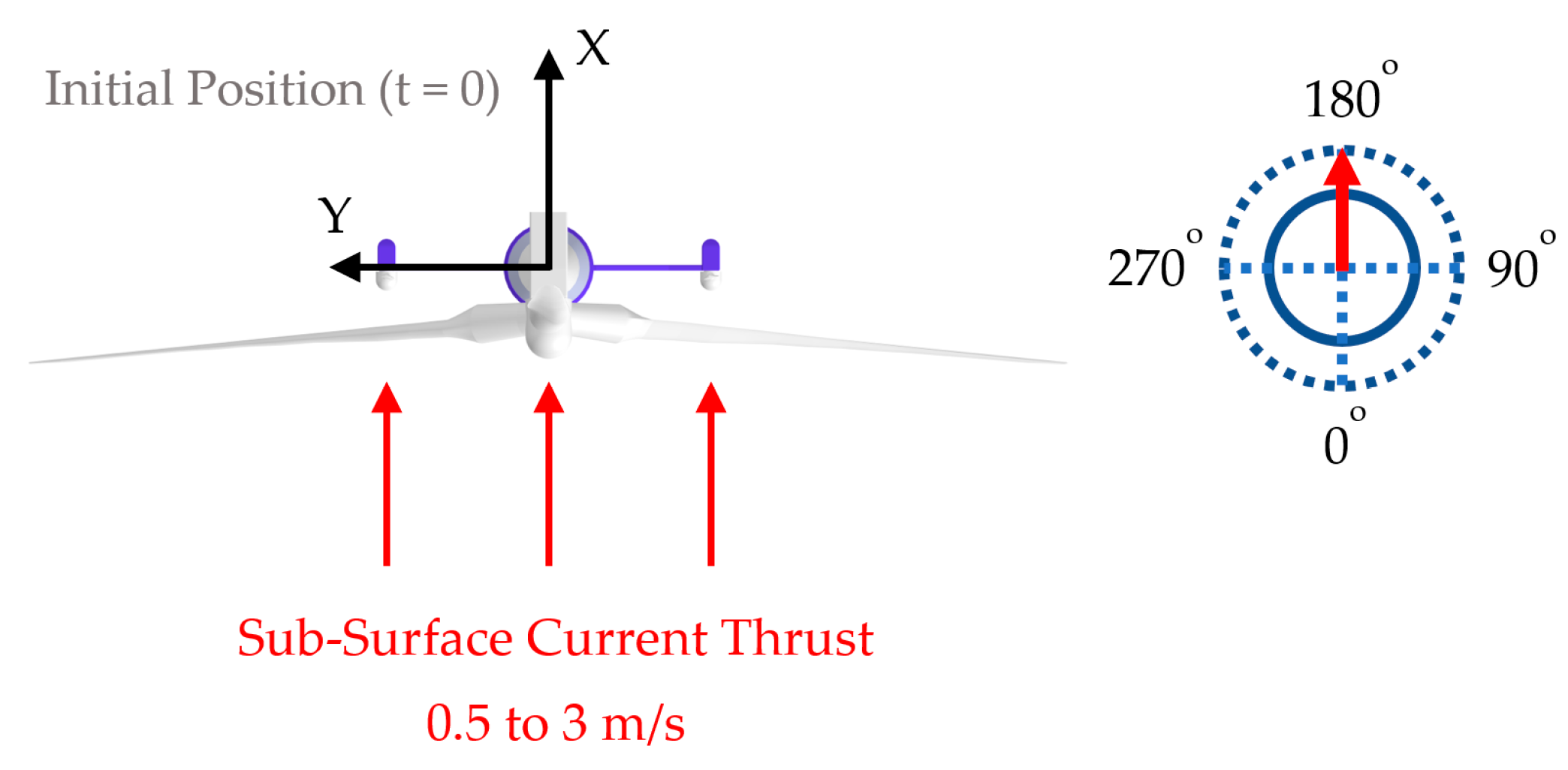
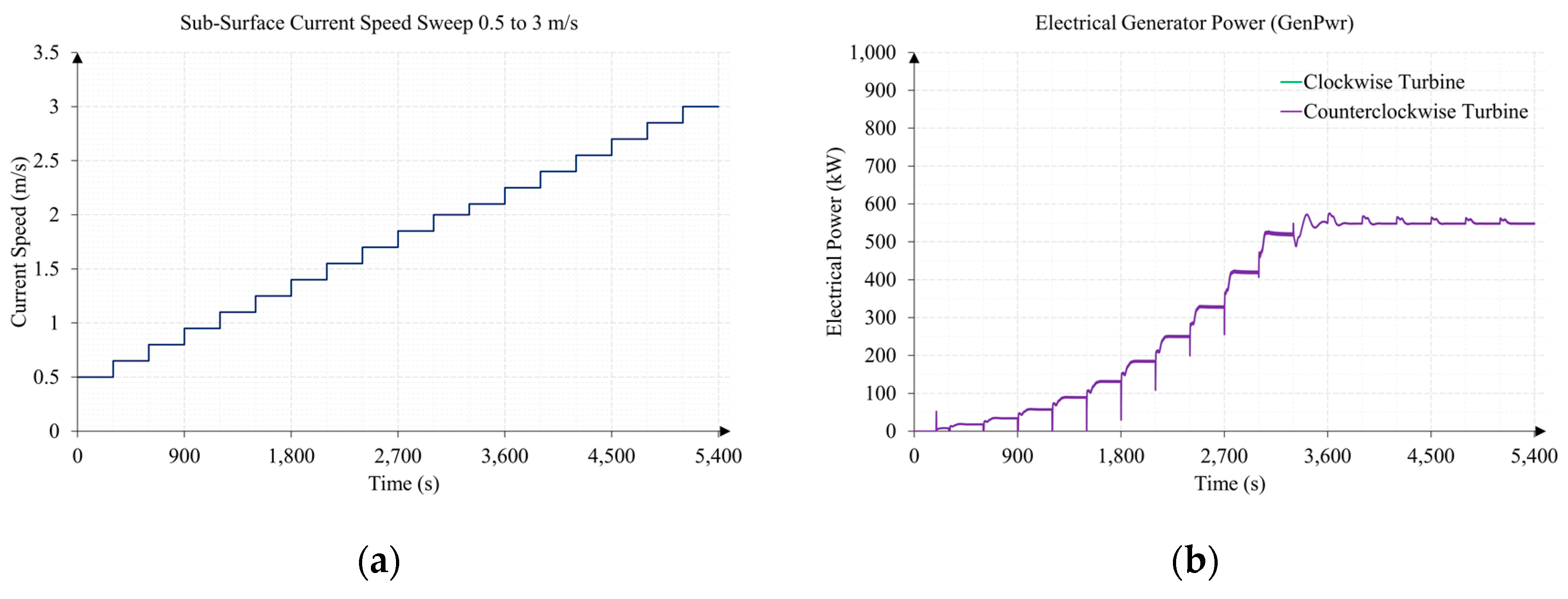
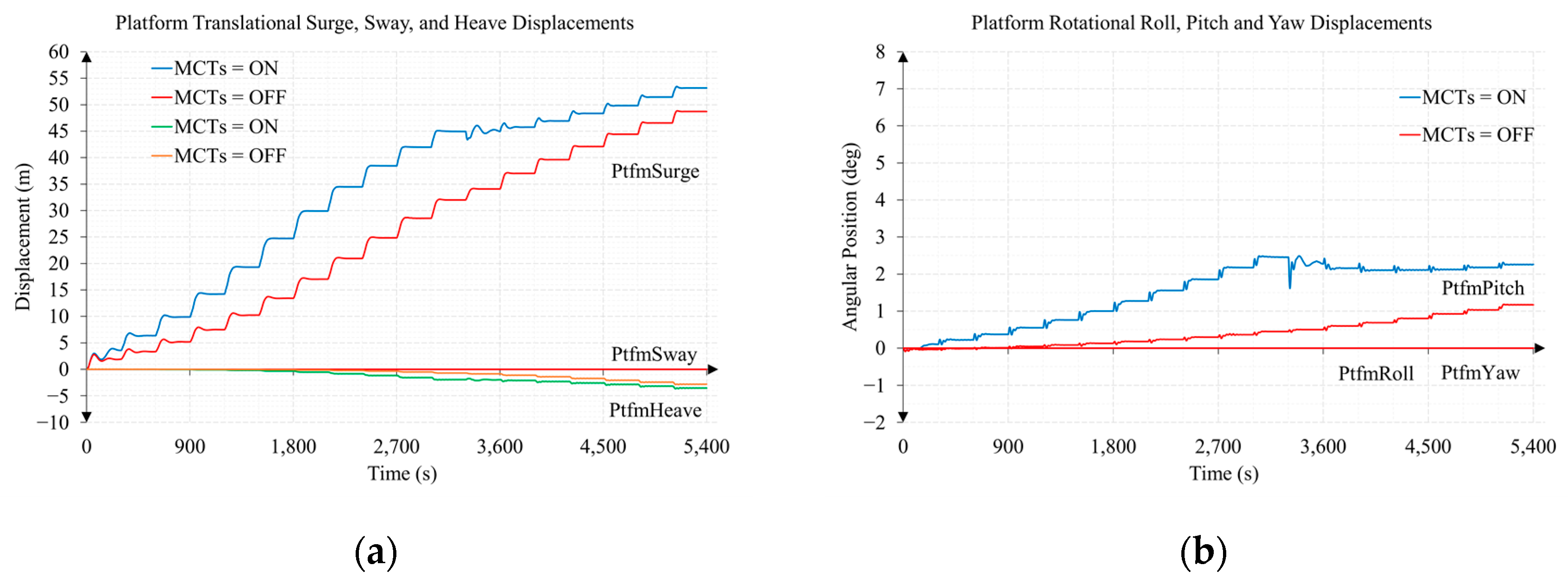
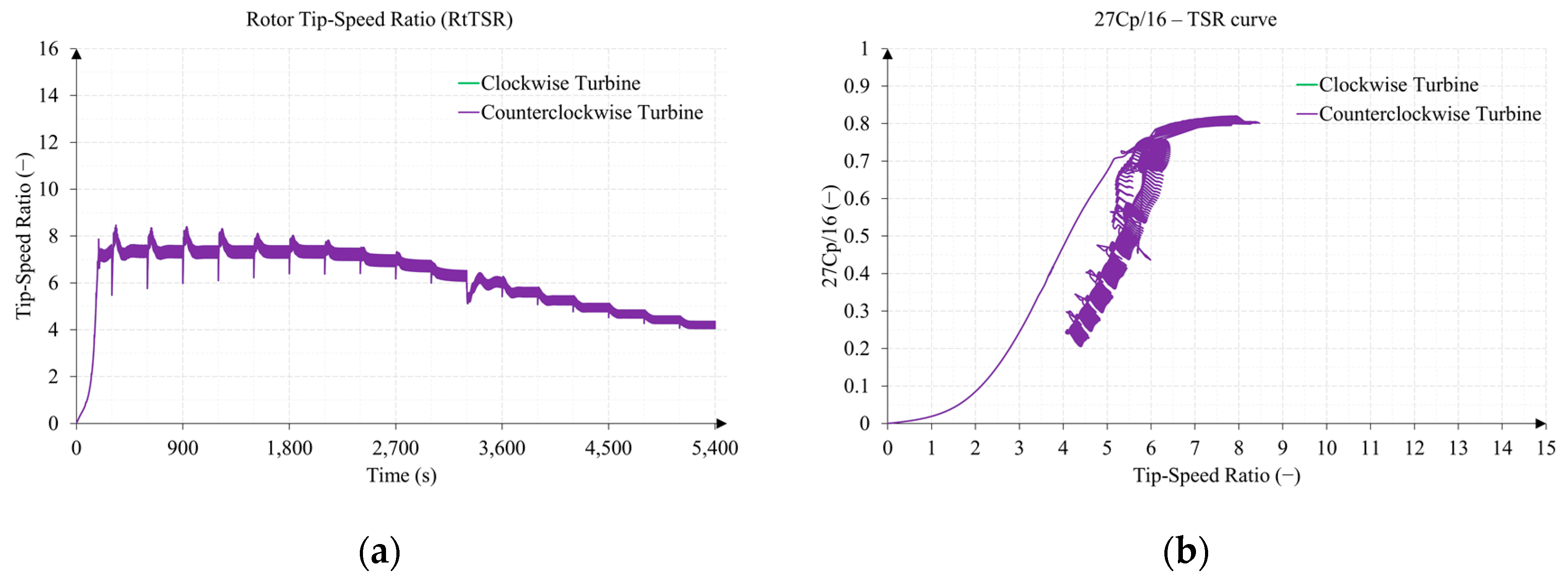
3.2. Test 2. Sub-Surface Current Speed Sweep from 0.5 to 3 m/s

Figure 21 shows the configuration of Test 2, in which a sweep of sub-surface current speeds was made from 0.5 to 3 m/s, with a direction of zero degrees, a wind speed of 0 m/s, and without the presence of waves.
As shown in Figure 21, Test 2 uses the complete mathematical model of the floating hybrid system made up of the three turbines (as shown in Figure 1), although in this case, the wind turbine was stopped due to the absence of wind.
As can be seen in Figure 22a, the sweep of sub-surface current speeds ( V S W L ) is carried out in two sections. The first from 0.5 to 2 m/s, and the second from 2.1 to 3 m/s. In each of them, the speed also increased by 0.15 m/s every 300 s.
Figure 22b shows a graph of the electrical power generated, in which it reached the maximum power from a sub-surface current speed of approximately 2 m/s.
Figure 23 shows the graphs of the different degrees of freedom of the floating hybrid system, but in this case, two simulations were included under the same conditions: one with the turbines running and generating power, and another in which the turbines are stopped. This is because the density of the fluid, in this case seawater, is almost a thousand times greater than that of air, so the interaction of the sub-surface current on the floating platform is by no means negligible.
When analyzing Figure 23, it can be deduced that most of the displacements produced did not come from the thrust of the MCTs, but rather from the effect of the sub-surface current on the floating platform.
Figure 24 shows the two magnitudes that control the MCTs as well as their relationship with the rotor aerodynamic torque and the rotor speed of the turbine.
Figure 24 shows three of the magnitudes that can be compared with the results presented in [34,35], with this comparison proving satisfactory. These are the rotor aerodynamic torque, the collective blade pitch angle, and the rotor speed of the turbine.
Figure 25 shows, in this case, the relationship between the rotor thrust exerted by the MCTs and the rotor aerodynamic power present in the low-speed shaft with their respective coefficients.
Figure 26a shows another magnitude that can be satisfactorily compared with the results presented in [34,35], the tip-speed ratio. Figure 26b shows the 27 C P / 16 T S R curve in which a maximum efficiency of MCTs around 0.8 was observed.
Finally, Figure 27 shows the control actions of the generator torque and collective blade pitch angle controllers.
The reasoning described in the previous section for Test 1 is extensible for the interpretation of most of the graphs represented in this section. However, it is interesting to verify the operation of the MCTs as a result of the application of the gain scheduled of the two controllers shown in Table 12 and Table 13.
In the graphs in which the results are indicated for the clockwise turbine and for the counterclockwise turbine, only one line appeared because the results were superimposed. This was due to the orientation of the current with respect to the floating hybrid system (see Figure 21), which caused mooring lines 2 and 3 to act symmetrically (see mooring lines numbering in Figure 14). This situation was also caused by the fact that the marine current turbines rotated in opposite directions, counteracting the moments produced in each of them (see Figure 13). This did not occur in Test 1 since the wind turbine only rotated clockwise, causing increases in the sway and roll degrees of freedom as seen in Figure 16.
Using FHYGSYS, more magnitudes can be plotted such as the angle of attack ( φ A t t a c k   ( A V ) ( t ) ), the axial induction factor ( a x i f ( A V ) ( t ) ), and the angular induction factor ( a n i f ( A V ) ( t ) ), which are obtained through Equations (73) to (75), respectively.

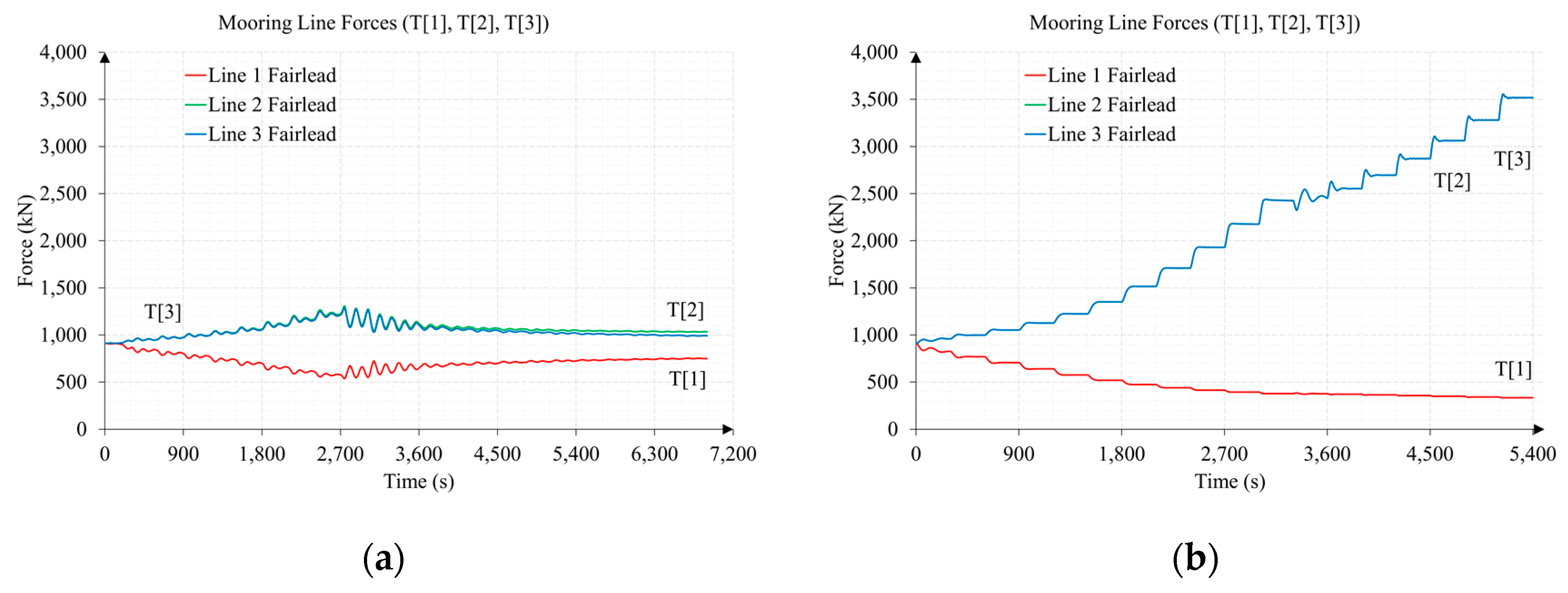
3.3. Comparison of Mooring Line Tensions between Tests 1 and 2

Concluding the presentation of results, it is interesting to highlight the behavior of the mooring system in each of the tests performed. Figure 28 shows the tensions in the fairleads of the mooring lines in both cases.
Figure 28b shows that mooring lines 2 and 3 suffered much higher tensions in Test 2 than those in Test 1. This was mainly due, as seen in Figure 23a, to the thrust caused by the sub-surface current on the platform floating. This is an effect that occurs in spar-buoy type systems. In other concepts such as the semisubmersible floating system [52], this problem is minimized.
In Test 2, the graphs of mooring lines 2 and 3 appeared superimposed by the symmetries produced and explained in the previous section. While differences were observed in the same mooring lines of Test 1 (Figure 28a), this was because there was only one turbine that rotated clockwise in Test 1, causing a moment that was not countered.
In Test 1, it was also observed that when there was a decrease in thrust—around 2700 s—the tension in mooring lines 2 and 3 decreased, and increased in mooring line 1.

4. Discussion

This work presents the modeling of the turbines of a floating hybrid system—wind and two marine current turbines (see Figure 1)—using the BEM theory, integrating this modeling in the FHYGSYS tool.
It was possible to obtain a reliable mathematical model since the version of OC3-Hywind implemented in FHYGSYS has been validated through a code-to-code comparison with simulations carried out under the same conditions with FASTv8. Appendix B shows the comparison of results for two wind speeds: 11 and 15 m/s. Similar comparisons were made for all of the wind speeds in Test 1, obtaining results with a precision similar to that presented in the results in Appendix B.
The operating results of the marine current turbines shown in Section 3.2 using the floating hybrid system model shown in Figure 1 were also validated by comparing the results obtained with the magnitudes available in [34,35].
The results presented in Section 3 also allow us to deepen our understanding of the operation of wind and marine current turbines over their entire working range, thanks to the number of magnitudes for which information is available.
Analyzing the results presented in Section 3, it was observed that at low speeds, logically, the power generated was low. It was also observed that until the turbines reached their rated rotor speed, as the fluid velocity increased, so did the power and thrust exerted by the turbines. Once the rated rotor speed was reached, the pitch angle controller came into operation and from that situation, as the fluid speed increased, the power stabilized, progressively lowering the thrust exerted by the turbines. This is an example of the great influence that the blade pitch angle has on the aerodynamic or hydrodynamic behavior of the turbines.
Another issue to highlight from the results is the influence of the sub-surface current on the floating platform (spar-buoy), since, as can be seen in Figure 23, the greatest percentage of the thrust on the floating hybrid system is not caused by the marine current turbines. In fact, in this figure, it can be seen that when the rated rotor speed was reached at around 3300 s, the thrust on the floating system decreased due to the reduction in the thrust of the marine turbines. This issue forces the mooring system to suffer high tensions for which it must be correctly sized. There is also the possibility of studying the use of other concepts of floating wind turbines that minimize this problem such as the semisubmersible floating system [52].
The incorporation of the modeling of the turbines using the BEM theory allows, for example, to study the behavior of these at start-up when they are stopped. However, one of the most important issues achieved with this work is having the possibility of designing different control systems simply by replacing the control system shown in Figure 9 with a different one.
In this work, a first control system was developed based on two PID controllers that control the rotor speed of the turbine by controlling the generator torque and controlling the collective blade pitch angle. Because the floating hybrid system presents a clearly nonlinear behavior, a gain scheduled was implemented for the torque and pitch PID controllers of the wind turbine and the marine current turbines. This is a relatively simple control system with which the speed of the turbines is controlled. When the three turbines are running, the controllers operate simultaneously but not in a coordinated manner.
For this reason, future works will address cooperative control strategies that allow for the establishment of coordinated control actions in order to optimize the energy performance and the structural stability of the floating hybrid system. Based on this idea and using FHYGSYS, multivariable control systems—multi-input multi-output (MIMO) systems—can be designed, thus improving the operation of the floating hybrid system. In addition, control strategies can also be designed that allow for the use of marine current turbines as actuation elements, making them work as a twin propulsion system actuator, to help in the stability of the system in adverse weather conditions.
As with the control system, the modeling of the actuators that intervene on the floating hybrid system can also be modified (see Figure 9). This allows for the application of other approaches different from the one described in Section 2.4 for the modeling of the actuators.
Another important possibility offered by turbine modeling using BEM theory is to predict the behavior of turbines for which operating data are not available. This allows future works to evaluate other marine current turbine designs with different dimensions, different hydrodynamic profiles, etc.
Finally, it is intended to conclude this series of works describing the mathematical model implemented in FHYGSYS from the point of view of the computer techniques used.

Supplementary Materials

The following supporting information can be downloaded at: https://www.mdpi.com/article/10.3390/jmse11081634/s1, Video S1: Test B1; Video S2: Test B2.

Author Contributions

Conceptualization, E.G.; Methodology, F.T and E.G.; Software, F.T.; Validation, F.T., E.G., A.C. and E.Q.; Formal analysis, F.T., E.G. and E.Q.; Investigation, E.G., E.Q., A.C. and F.T.; Resources, F.T. and A.C.; Data curation, F.T., E.G., E.Q. and A.C.; Writing—original draft preparation, F.T. and E.G.; Writing—review and editing, F.T., E.G., E.Q. and A.C.; Visualization, E.G., F.T. and E.Q.; Supervision, E.G., E.Q. and A.C.; Project administration, E.G., E.Q. and A.C.; Funding acquisition, E.G. and E.Q. All authors have read and agreed to the published version of the manuscript.

Funding

Funding for open access charge: Vicerrectorado de Investigación de la Universitat Politècnica de València (PAID-11-22).

Institutional Review Board Statement

Not applicable.

Informed Consent Statement

Not applicable.

Data Availability Statement

Not applicable.

Acknowledgments

Funding for open access charge: Universitat Politècnica de València.

Conflicts of Interest

The authors declare no conflict of interest.

Abbreviations

Acronym list
ANSYSSwanson Analysis Systems
BEMBlade Element Momentum theory
CFDComputational Fluid Dynamics
DOFDegrees Of Freedom
FASTFatigue, Aerodynamics, Structures, and Turbulence
FHYGSYS Floating Hybrid Generator SYstems Simulator
HAWC2Horizontal Axis Wind turbine simulation Code 2nd generation
HAWTHorizontal Axis Wind Turbine
MCTMarine Current Turbines
MIMOMulti-Input Multi-Output
NRELNational Renewable Energy Lab
OC3Offshore Code Comparison Collaboration
OLAFcOnvecting LAgrangian Filaments
OWTOffshore Wind Turbines
PIDProportional–Integral–Derivative
PLCProgrammable Logic Controller
RTHSReal-Time Hybrid Simulation
SHYFEMSystem of HYdrodynamic Finite Element Modules
SOWFASimulator for Wind Farm Applications
WRPWAMIT Reference Point
Symbol List
a n i f ( t ) angular induction factor of the wind turbine (or marine current turbine)
a n i f ( A V ) ( t ) mean value of angular induction factor
A T u r b i n e area of the wind turbine (or marine current turbine)
a x i f ( t ) axial induction factor of the wind turbine (or marine current turbine)
a x i f ( A V ) ( t ) mean value of axial induction factor
a x i f m a x value of Glauert correction whose value is 1/3
α r o t o r ( t ) low-speed shaft angular acceleration of the turbine rotor
α power law exponent
C D aerodynamic (or hydrodynamic) drag coefficient
C L aerodynamic (or hydrodynamic) lift coefficient
C N θ ( t ) aerodynamic (or hydrodynamic) normal coefficient
center of mass of the wind turbine
C o M W T u r b i n e   ( B O D Y ) ( t ) center of mass of the wind turbine expressed in the mobile coordinate system
C P ( t ) power coefficient
C T ( t ) thrust coefficient
C T θ ( t ) aerodynamic (or hydrodynamic) tangential coefficient
D ( h ) tower diameter to calculate the vector v   W I N D   t o w e r s h a d o w     ( B O D Y ) ( h )
Δ z p n i   ( M C T ) value that   corrects   the   Z   component   of   the   p n i   ( M C T ) ( t ) To calculate the shadow effect in a marine current turbine
d F   b l a d e   i j   ( B O D Y ) ( t ) resultant of the differential forces of blade element i of blade j expressed in the mobile coordinate system
differential of thrust force
differential of thrust force of blade element i of blade
d F   t h r u s t   i j   ( B O D Y ) ( t ) differential of thrust force vector of blade element i of blade j expressed in the mobile coordinate system
d F t o r q u e differential of torque force
d F t o r q u e   i j ( t ) differential of torque force of blade element of blade j
d F   t o r q u e   i j   ( B O D Y ) ( t ) differential of torque force vector of blade element i of blade expressed in the mobile coordinate system
d M   b l a d e   i j   ( B O D Y ) ( t ) resultant of the differential moments of blade element i of blade j expressed in the mobile coordinate system
d M p i t c h i n g differential of pitching moment
d p n i blade elements or blade differentials
δ direction of the wind velocity vector
e ( t ) error value of a PID controller
ε direction of the sub-surface current velocity vector
ε a value   of   the   percent   relative   error   to   calculate   the   values   of   a x i f ( t ) and a n i f ( t )
ε a m i n minimum value of the percent relative error whose value is 5 · 10 9
F   b l a d e   j   ( B O D Y ) ( t ) resultant of the forces of blade j expressed in the mobile coordinate system
F c e n t e r s h a d o w factor that represents the shadow effect of the central tube of the marine current support
F d o w n s h a d o w factor that represents the shadow effect of the lower tube of the marine current support
F H u b l o s s ( t ) hub-loss factor
F k ( B O D Y )   W I N D   T U R B I N E ( t ) vector of wind turbine forces and moments expressed in the mobile coordinate system
F l o s s ( t ) total turbine losses
F t h r u s t thrust force
F   T h r u s t   ( B O D Y ) ( t ) total thrust vector produced by the wind turbine expressed in the mobile coordinate system
F T i p l o s s ( t ) Prandtl’s tip-loss factor
F t o r q u e torque force
F T r i g g pitch controller trigger offset factor
F T r i g g ( % ) trigger offset factor
F u p s h a d o w factor that represents the shadow effect of the upper tube of the marine current support
i symbol to refer to a specific blade element
I r o t o r total inertia of the wind turbine rotor
I W T u r b i n e wind turbine moment of inertia about this x axis ( I W T x x )
I M C T u r b i n e marine current turbine moment of inertia about this x axis ( I M C T x x )
I M C T u r b i n e   ( S U M ) marine current turbine moment of inertia about this x axis ( I M C T x x   ( S U M ) ) to calculate added mass
I W T x x , I W T y y , I W T z z wind turbine moments of inertia
I M C T x x , I M C T y y , I M C T z z marine current turbine moments of inertia
I M C T x x   ( S U M ) , I M C T y y   ( S U M )   I M C T z z   ( S U M ) marine current turbine moments of inertia to calculate added mass
j symbol to refer to a specific blade
K a n i f ( t ) term of a n i f ( t ) equation
K a x i f ( t ) term of a x i f ( t ) equation
K p proportional gain of a PID controller
K p G E N proportional gain of the torque PID controller
K p P i t c h proportional gain of the collective blade pitch angle PID controller
L C h o r d chord length of a blade element
M B O D Y I N E R T I A L transformation matrix that allows changing between the inertial coordinate system and the mobile coordinate system
M   a e r o   ( B O D Y ) ( t ) total moment caused by the aerodynamics on the turbine
M a e r o s h a f t ( t ) low-speed shaft aerodynamic torque or moment (torque) about the shaft of the turbine
M   b l a d e   ( B O D Y ) ( t ) moment vector caused by the blades on a turbine
M   b l a d e   j   ( B O D Y ) ( t ) resultant of the moments of blade j expressed in the mobile coordinate system
M G E N ( t ) high-speed shaft generator torque
M G E N s h a f t ( t ) low-speed shaft generator torque
M   h u b   ( B O D Y ) ( t ) total moment vector originated by the force vector from the bases of the blades to the center of mass of the turbine
M   h u b   j   ( B O D Y ) ( t ) moment vector originated by the force vector F   b l a d e   j   ( B O D Y ) ( t ) from the bases of the blades to the center of mass of the turbine
M H T   B O D Y I N E R T I A L homogeneous transformation matrix that allows for changing between the inertial coordinate system and the mobile coordinate system
M I T   ( W T u r b i n e ) wind turbine rotor inertia tensor
M I T   ( M C T u r b i n e ) marine current turbine rotor inertia tensor
M I T   ( M C T u r b i n e   ( S U M ) ) marine current turbine rotor inertia tensor to calculate added mass
M p i t c h resultant of pitching moment on a turbine
pitching moment
M   p i t c h i n g   ( B O D Y ) ( t ) total pitching moment vector
M p i t c h i n g   j ( t ) pitching moment originated in blade j
M   p i t c h i n g   j   ( B O D Y ) ( t ) pitching moment vector originated in blade j expressed in the mobile coordinate system
M r o t o r ( t ) low-speed shaft torque
M   r o t o r   ( B O D Y ) ( t ) low-speed shaft torque vector expressed in the mobile coordinate system
M   T h r u s t   ( B O D Y ) ( t ) total moment vector produced by the wind turbine at the origin of the mobile coordinate system expressed in the same coordinate system
M   T h r u s t   j   ( B O D Y ) ( t ) moment produced by the resultant of the forces of blade j at the origin of the mobile coordinate system expressed in the same coordinate system
difference   between   the   angular   speed   to   be   reached   ( )   and   the   high - speed   shaft   angular   speed   ( )
ω G E N ( t ) high-speed shaft angular speed of the generator
ω r o t o r ( t ) low-speed shaft angular speed of the turbine rotor
Ω r o t o r ( t ) low-speed shaft angular speed of the turbine rotor expressed in rpm
Ω S P ( t ) set point of low-speed shaft angular speed expressed in rpm
ω S P set point of high-speed shaft angular speed
P A E R O ( t ) rotor aerodynamic power
P E L E ( t ) electrical generator power
P M E C ( t ) mechanical power or low-speed shaft power
p n i center of each of the blade elements
p n i ( B L A D E ) center of each of the blade elements expressed in a blade coordinate system
p n i ( B O D Y ) center of each of the blade elements expressed in the mobile coordinate system
p n i ( I N E R T I A L ) center of each of the blade elements expressed in the inertial coordinate system
p n 0 j   ( B O D Y ) ( t ) center point at the base of blade j
p n i j   ( B O D Y ) ( t ) center of blade element i of blade j expressed in the mobile coordinate system
φ A t t a c k ( t ) angle   of   attack   between   velocity   V r e l ( t ) and the chord line of each blade element
φ A t t a c k   ( A V ) ( t ) mean value of angle of attack
φ P i t c h ( t ) collective blade pitch angle
φ T w i s t twist angle of a blade element
ψ r o t o r ( t ) angular position of the turbine rotor
Q a e r o ( t ) magnitude of vector
r T u r b i n e turbine radius
R t A e r o F total rotor aerodynamic forces (thrust)
R t A e r o M total rotor aerodynamic moments (torque)
ρ A I R density of air whose value is 1.225   kg / m 3
ρ S E A   W A T E R density of seawater whose value is
σ i local solidity
T d derivative time of a PID controller
integration time of a PID controller
T i G E N integration time of the torque PID controller
T i P i t c h integration time of the collective blade pitch angle PID controller
T T h r u s t ( t ) magnitude of vector F   T h r u s t   ( B O D Y ) ( t )
T S R ( t ) tip-speed ratio
θ ( t ) angle between V r e l ( t ) velocity and a blade vertical plane
u ( t ) control action of a PID controller
u M G E N ( t ) control action of the torque PID controller
u P i t c h ( t ) control action of the collective blade pitch angle PID controller
u   B j   t h r u s t thrust   unit   vector   or   vector   perpendicular   to   blade   j
u   B j   t h r u s t   ( B O D Y ) thrust   unit   vector   or   vector   perpendicular   to   blade   expressed in the mobile coordinate system
u   B j   t o r q u e   ( B O D Y ) torque unit vector expressed in the mobile coordinate system
pitching   moment   unit   vector   of   blade   j
u   M j   p i t c h i n g   ( B O D Y ) pitching   moment   unit   vector   of   blade   j expressed in the mobile coordinate system
u   s h a f t shaft unit vector
u   s h a f t   ( B O D Y ) shaft unit vector expressed in the mobile coordinate system
V 0 ( t ) or V 0   i j ( t ) magnitude of vector v   n i   E F F B j   t h r u s t ( B O D Y ) ( t )
V 0   ( A V ) ( t ) mean of the magnitude of the effective wind velocity vector
V 1 2 ( t ) normal velocity to the vertical plane of each blade
V r e l ( t ) magnitude of the wind velocity reaching each blade element
V r o t ( t ) tangential velocity to the vertical plane of each blade
V W R E F magnitude—or mean wind speed—of the wind velocity vector at the reference height
V W I N D ( h ) wind   speed   at   the   height   of   the   center   point   of   each   blade   element   ( p n i )
v   n i   E F F B j   t h r u s t ( B O D Y ) ( t ) effective wind velocity vector at node i   of   blade   j expressed in the mobile coordinate system
v   n i   E F F W I N D ( B O D Y ) ( h , t ) effective wind velocity vector at node i expressed in the mobile coordinate system
v   p n i   ( B O D Y ) ( t ) velocity   vector   of   the   center   point   of   each   blade   element   ( p n i ) expressed in the mobile coordinate system
v   p n i   ( I N E R T I A L ) ( t ) velocity   vector   of   the   center   point   of   each   blade   element   ( p n i ) expressed in the inertial coordinate system
v   S S C U R ( B O D Y ) ( h ) sub-surface current velocity vector of the vector field rotated by the corresponding angle ε expressed in the mobile coordinate system
v   S S C U R   s u p p o r t s h a d o w     ( B O D Y ) ( h ) sub-surface current velocity vector considering the support shadow effect
v   W I N D ( B O D Y ) ( h ) wind velocity vector of the vector field rotated by the corresponding angle δ expressed in the mobile coordinate system
v   W I N D ( I N E R T I A L ) ( h ) wind velocity vector of the vector field rotated by the corresponding angle δ expressed in the inertial coordinate system
v   W I N D   t o w e r s h a d o w     ( B O D Y ) ( h ) wind velocity vector considering the tower shadow effect
x p n i ,   y p n i ,   z p n i x, y and z components of p n i ( B O D Y ) ( t ) point
x p n i   ( M C T ) ,   y p n i   ( M C T ) ,   z p n i   ( M C T ) x, y and z components of p n i ( M C T ) ( t ) point
z R E F reference height of the wind velocity vector
z W I N D ( t ) height to calculate the magnitude of the wind velocity vector

Appendix A

This appendix presents the central points ( p n i ) of each blade element as well as the points that allow for the calculation of the unit vectors associated with the blades and used on multiple occasions throughout this work. Table A1 shows the central points of the wind turbine blades. The points expressed in the mobile coordinate system are in their initial position for a wind direction ( δ ) equal to zero degrees.
Table A1. Central points of the wind turbine blades.
Node p n i ( B L A D E )   ( m ) p n i ( B O D Y )   ( m )
(Blade 1)
p n i ( B O D Y )   ( m )
(Blade 2)
p n i ( B O D Y )   ( m )
(Blade 3)
0 (blade base)(0, 0, 0)(−5.126, 0, 91.52)(−5.322, −1.299, 89.28)(−5.322, 1.299, 89.28)
1(0, 0, 1.3667)(−5.067, 0, 92.88)(−5.441, −2.482, 88.60)(−5.441, 2.482, 88.60)
2(0, 0, 4.1)(−4.948, 0, 95.61)(−5.679, −4.846, 87.25)(−5.679, 4.846, 87.25)
3(0, 0, 6.8333)(−4.828, 0, 98.34)(−5.917, −7.211, 85.90)(−5.917, 7.211, 85.90)
4(0, 0, 10.25)(−4.679, 0, 101.8)(−6.214, −10.17, 84.21)(−6.214, 10.17, 84.21)
5(0, 0, 14.35)(−4.500, 0, 105.9)(−6.571, −13.72, 82.19)(−6.571, 13.72, 82.19)
6(0, 0, 18.45)(−4.322, 0, 110.0)(−6.927, −17.26, 80.16)(−6.927, 17.26, 80.16)
7(0, 0, 22.55)(−4.143, 0, 114.1)(−7.284, −20.81, 78.14)(−7.284, 20.81, 78.14)
8(0, 0, 26.65)(−3.964, 0, 118.1)(−7.641, −24.36, 76.12)(−7.641, 24.36, 76.12)
9(0, 0, 30.75)(−3.785, 0, 122.2)(−7.997, −27.90, 74.09)(−7.997, 27.90, 74.09)
10(0, 0, 34.85)(−3.606, 0, 126.3)(−8.354, −31.45, 72.07)(−8.354, 31.45, 72.07)
11(0, 0, 38.95)(−3.427, 0, 130.4)(−8.711, −35.00, 70.04)(−8.711, 35.00, 70.04)
12(0, 0, 43.05)(−3.249, 0, 134.5)(−9.067, −38.55, 68.01)(−9.067, 38.55, 68.01)
13(0, 0, 47.15)(−3.070, 0, 138.6)(−9.424, −42.09, 65.99)(−9.424, 42.09, 65.99)
14(0, 0, 51.25)(−2.891, 0, 142.7)(−9.781, −45.64, 63.97)(−9.781, 45.64, 63.97)
15(0, 0, 54.6667)(−2.742, 0, 146.1)(−10.08, −48.60, 62.28)(−10.08, 48.60, 62.28)
16(0, 0, 57.4)(−2.623, 0, 148.9)(−10.32, −50.96, 60.93)(−10.32, 50.96, 60.93)
17(0, 0, 60.1333)(−2.503, 0, 151.6)(−10.55, −53.33, 59.58)(−10.55, 53.33, 59.58)
18 (blade tip)(0, 0, 61.5)(−2.444, 0, 153.0)(−10.67, −54.51, 58.91)(−10.67, 54.51, 58.91)
19 (Surge positive unit)(1, 0, 0)(−4.127, 0, 91.47)(−4.329, −1.337, 89.17)(−4.329, 1.337, 89.17)
20 (Sway negative unit)(0, −1, 0)(−5.126, −1, 91.52)(−5.398, −0.7990, 88.41)(−5.247, 1.799, 90.14)
21 (Heave positive unit)(0, 0, 1)(−5.082, 0, 92.52)(−5.409, −2.164, 88.78)(−5.409, 2.164, 88.78)
The calculation of the unit vectors u   B j   t h r u s t , u   B j   t o r q u e , and u   M j   p i t c h i n g was carried out using Equations (A1)–(A3), respectively.
u   B j   t h r u s t = p n 19   ( B O D Y ) p n 0   ( B O D Y )
u   B j   t o r q u e = p n 20   ( B O D Y ) p n 0   ( B O D Y )
u   M j   p i t c h i n g = p n 21   ( B O D Y ) p n 0   ( B O D Y )
These points rotate along with the blades and the subtraction at each moment produces the unit vector in the desired direction.
Figure A1 shows the floating hybrid system in its initial position as well as the numbering of each blade.
Figure A1. Floating hybrid system in its initial position.
Jmse 11 01634 g0a1
Table A2 shows the central points of the clockwise marine current turbine blades. The points expressed in the mobile coordinate system are in their initial position for a sub-surface current direction ( ε ) equal to zero degrees.
Table A2. Central points of the clockwise marine current turbine blades.
Node p n i ( B L A D E )   ( m ) p n i ( B O D Y )   ( m )
(Blade 1)
p n i ( B O D Y )   ( m )  
(Blade 2)
0 (blade base)(−1.1, 0, 0)(−0.9, 17.1, −19)(−0.9, 17.1, −21)
1(−1.1, 1.075, 0)(−0.9, 17.1, −18.93)(−0.9, 17.1, −21.08)
2(−1.1, 1.3607, 0)(−0.9, 17.1, −18.639)(−0.9, 17.1, −21.36)
3(−1.1, 1.7821, 0)(−0.9, 17.1, −18.22)(−0.9, 17.1, −21.78)
4(−1.1, 2.2036, 0)(−0.9, 17.1, −17.80)(−0.9, 17.1, −22.20)
5(−1.1, 2.625, 0)(−0.9, 17.1, −17.38)(−0.9, 17.1, −22.63)
6(−1.1, 3.1342, 0)(−0.9, 17.1, −16.87)(−0.9, 17.1, −23.13)
7(−1.1, 3.7313, 0)(−0.9, 17.1, −16.27)(−0.9, 17.1, −23.73)
8(−1.1, 4.3283, 0)(−0.9, 17.1, −15.67)(−0.9, 17.1, −24.32)
9(−1.1, 4.9253, 0)(−0.9, 17.1, −15.08)(−0.9, 17.1, −24.93)
10(−1.1, 5.5223, 0)(−0.9, 17.1, −14.48)(−0.9, 17.1, −25.52)
11(−1.1, 6.1193, 0)(−0.9, 17.1, −13.88)(−0.9, 17.1, −26.12)
12(−1.1, 6.7164, 0)(−0.9, 17.1, −13.28)(−0.9, 17.1, −26.72)
13(−1.1, 7.3134, 0)(−0.9, 17.1, −12.69)(−0.9, 17.1, −27.31)
14(−1.1, 7.9104, 0)(−0.9, 17.1, −12.09)(−0.9, 17.1, −27.91)
15(−1.1, 8.5074, 0)(−0.9, 17.1, −11.49)(−0.9, 17.1, −28.51)
16(−1.1, 9.1045, 0)(−0.9, 17.1, −10.89)(−0.9, 17.1, −29.11)
17(−1.1, 9.7015, 0)(−0.9, 17.1, −10.30)(−0.9, 17.1, −29.70)
18 (blade tip)(−1.1, 0, 10)(−0.9, 17.1, −10)(−0.9, 17.1, −30)
19 (Surge positive unit)(−0.1, 0, 0)(0.1, 17.1, −19)(0.1, 17.1, −21)
20 (Sway negative unit)(−1.1, −1, 0)(−0.9, 16.1, −19)(−0.9, 18.1, −21)
21 (Heave positive unit)(−1.1, 0, 1)(−0.9, 17.1, −18)(−0.9, 17.1, −22)
Table A3 shows the central points of the counterclockwise marine current turbine blades. The points expressed in the mobile coordinate system are in their initial position for a sub-surface current direction ( ε ) equal to zero degrees.
Table A3. Central points of the counterclockwise marine current turbine blades.
Node p n i ( B L A D E )   ( m ) p n i ( B O D Y )   ( m )
(Blade 1)
p n i ( B O D Y )   ( m )
(Blade 2)
0 (blade base)(−1.1, 0, 0)(−0.9, −17.1, −19)(−0.9, −17.1, −21)
1(−1.1, 1.075, 0)(−0.9, −17.1, −18.93)(−0.9, −17.1, −21.08)
2(−1.1, 1.3607, 0)(−0.9, −17.1, −18.639)(−0.9, −17.1, −21.36)
3(−1.1, 1.7821, 0)(−0.9, −17.1, −18.22)(−0.9, −17.1, −21.78)
4(−1.1, 2.2036, 0)(−0.9, −17.1, −17.80)(−0.9, −17.1, −22.20)
5(−1.1, 2.625, 0)(−0.9, −17.1, −17.38)(−0.9, −17.1, −22.63)
6(−1.1, 3.1342, 0)(−0.9, −17.1, −16.87)(−0.9, −17.1, −23.13)
7(−1.1, 3.7313, 0)(−0.9, −17.1, −16.27)(−0.9, −17.1, −23.73)
8(−1.1, 4.3283, 0)(−0.9, −17.1, −15.67)(−0.9, −17.1, −24.32)
9(−1.1, 4.9253, 0)(−0.9, −17.1, −15.08)(−0.9, −17.1, −24.93)
10(−1.1, 5.5223, 0)(−0.9, −17.1, −14.48)(−0.9, −17.1, −25.52)
11(−1.1, 6.1193, 0)(−0.9, −17.1, −13.88)(−0.9, −17.1, −26.12)
12(−1.1, 6.7164, 0)(−0.9, −17.1, −13.28)(−0.9, −17.1, −26.72)
13(−1.1, 7.3134, 0)(−0.9, −17.1, −12.69)(−0.9, −17.1, −27.31)
14(−1.1, 7.9104, 0)(−0.9, −17.1, −12.09)(−0.9, −17.1, −27.91)
15(−1.1, 8.5074, 0)(−0.9, −17.1, −11.49)(−0.9, −17.1, −28.51)
16(−1.1, 9.1045, 0)(−0.9, −17.1, −10.89)(−0.9, −17.1, −29.11)
17(−1.1, 9.7015, 0)(−0.9, −17.1, −10.30)(−0.9, −17.1, −29.70)
18 (blade tip)(−1.1, 0, 10)(−0.9, −17.1, −10)(−0.9, −17.1, −30)
19 (Surge positive unit)(−0.1, 0, 0)(0.1, −17.1, −19)(0.1, −17.1, −21)
20 (Sway negative unit)(−1.1, 1, 0)(−0.9, −16.1, −19)(−0.9, −18.1, −21)
21 (Heave positive unit)(−1.1, 0, −1)(−0.9, −17.1, −20)(−0.9, −17.1, −20)

Appendix B

To validate the mathematical model of the turbines using the BEM theory developed in this work, two tests are presented: the first with a wind speed ( V W R E F ) of 11 m/s in which, as indicated in Table 4, only the generator torque PID controller is in operation, and the second with a wind speed ( V W R E F ) of 15 m/s, in which, as indicated in Table 6 and explained in Section 2.4, both the generator torque PID controller and the collective blade pitch angle PID controller are in operation. Both tests do not include the effect of sub-surface currents or the effect of waves.
To carry out a code-to-code comparison between the results obtained with FHYGSYS and those obtained by FASTv8 under the same conditions, the version of OC3-Hywind implemented in FHYGSYS was used.
In this appendix, in all of the figures in which the results obtained using FHYGSYS were compared to those obtained with FASTv8 appear (Appendix B.1 and Appendix B.2), both the titles of the figures and the nomenclature included were the same as those used by FASTv8.

Appendix B.1. Test B1. Wind Speed 11 m/s and Direction 70 Degrees

The adjustment of the FASTv8 parameters to carry out a simulation with the same conditions as FHYGSYS, was the same as that indicated in the introduction of Appendix E in [36], with the differences shown in Table A4 and Table A5. In the Supplementary Materials, there is a video with the simulation of Test B1.
Table A4. Changes in “NRELOffshrBsline5MW_InflowWind_12mps.dat”.
SectionParameterOriginal ValueModified Value
PropagationDir0−70
Parameters for steady wind conditionsHWindSpeed011
Table A5. Changes in “NRELOffshrBsline5MW_OC3Hywind_ElastoDyn.dat”.
SectionParameterOriginal ValueModified Value
Initial conditionsRotSpeed11.890
NacYaw070
Figure A2 illustrates the orientation of the floating system toward the direction of the wind.
Figure A2. Test B1 conditions. Wind speed 11 m/s and direction of 70 degrees.
Jmse 11 01634 g0a2
Figure A3. Linear and angular degrees of freedom of Test B1: (a) linear degrees of freedom; (b) angular degrees of freedom.
Jmse 11 01634 g0a3
Figure A4. Torque and power of Test B1 yielded by the wind turbine modeling: (a) rotor aerodynamic torque; (b) rotor aerodynamic power; (c) low-speed shaft torque; (d) low-speed shaft power; (e) electrical generator torque; (f) electrical generator power.
Jmse 11 01634 g0a4
Figure A5. Thrust and rotor speed of Test B1 yielded by the wind turbine modeling: (a) rotor thrust; (b) rotor speed.
Jmse 11 01634 g0a5
Figure A6. Collective blade pitch angle and outstanding coefficients of Test B1 yielded by the wind turbine modeling: (a) blade pitch angle; (b) power coefficient; (c) tip-speed ratio; (d) thrust coefficient.
Jmse 11 01634 g0a6
Figure A7. Total integrated hydrodynamic loads from both the potential flow and strip theory at the WRP point and mooring system fairlead forces of Test B1: (a) surge and sway forces; (b) roll, pitch, and yaw moments; (c) heave force; (d) force on the fairleads of the floating platform of each mooring line. T[1], T[2], and T[3] are the nomenclature used by FASTv8 for the fairlead tensions in mooring lines 1, 2, and 3.
Jmse 11 01634 g0a7
In Figure A7, the WRP point (WAMIT reference point) is named; this point corresponds to the origin of the inertial coordinate system (see Figure 1) [53]. In Figure A4a and Figure A5a, the FASTv8 results shown corresponded to the modulus of the total rotor aerodynamic loads, where we applied Equation (A4) for Figure A4a and Equation (A5) for Figure A5a.
R t A e r o M = R t A e r o M x h 2 + R t A e r o M y h 2 + R t A e r o M z h 2
R t A e r o F = R t A e r o F x h 2 + R t A e r o F y h 2 + R t A e r o F z h 2

Appendix B.2. Test B2. Wind Speed 15 m/s and Direction 0 Degrees

As in the previous case, the adjustment of the FASTv8 parameters to carry out a simulation with the same conditions as with FHYGSYS was the same as that indicated in the introduction of Appendix E in [36], with the differences shown in Table A6 and Table A7. In the Supplementary Materials, there is a video with the simulation of Test B2.
Table A6. Changes in “NRELOffshrBsline5MW_InflowWind_12mps.dat”.
SectionParameterOriginal ValueModified Value
PropagationDir00
Parameters for steady wind conditionsHWindSpeed015
Table A7. Changes in “NRELOffshrBsline5MW_OC3Hywind_ElastoDyn.dat”.
SectionParameterOriginal ValueModified Value
Initial conditionsRotSpeed12.10
NacYaw00
Figure A8 shows the orientation of the floating system toward the direction of the wind.
Figure A8. Test B2 conditions. Wind speed 15 m/s and direction of 0 degrees.
Jmse 11 01634 g0a8
Figure A9. Linear and angular degrees of freedom of Test B2: (a) linear degrees of freedom; (b) angular degrees of freedom.
Jmse 11 01634 g0a9
Figure A10. Torque and power of Test B2 yielded by the wind turbine modeling: (a) rotor aerodynamic torque; (b) rotor aerodynamic power; (c) low-speed shaft torque; (d) low-speed shaft power; (e) electrical generator torque; (f) electrical generator power.
Jmse 11 01634 g0a10
Figure A11. Thrust and rotor speed of Test B2 yielded by the wind turbine modeling: (a) rotor thrust; (b) rotor speed.
Jmse 11 01634 g0a11
Figure A12. Collective blade pitch angle and outstanding coefficients of Test B2 yielded by the wind turbine modeling: (a) blade pitch angle; (b) power coefficient; (c) tip-speed ratio; (d) thrust coefficient.
Jmse 11 01634 g0a12
Figure A13. Total integrated hydrodynamic loads from both the potential flow and strip theory at the WRP point and mooring system fairlead forces of Test B2: (a) surge and sway forces; (b) roll, pitch, and yaw moments; (c) heave force; (d) force on the fairleads of the floating platform of each mooring line. T[1], T[2], and T[3] are the nomenclature used by FASTv8 for the fairlead tensions in mooring lines 1, 2, and 3.
Jmse 11 01634 g0a13

References

  1. Çengel, Y.A.; Cimbala, J.M. Fluid Mechanics: Fundamentals and Applications, 1st ed.; McGraw-Hill: New York, NY, USA, 2006. [Google Scholar]
  2. Hansen, M.O.L. Aerodynamics of Wind Turbines, 1st ed.; James & James Science Publishers, Ltd.: London, UK, 2000. [Google Scholar]
  3. Jonkman, J.M. Modeling of the UAE Wind Turbine for Refinement of FAST_AD.; NREL/TP-500-34755; NREL: Golden, CO, USA, 2003. [Google Scholar] [CrossRef]
  4. Burton, T.; Sharpe, D.; Jenkins, N.; Bossanyi, E. Wind Energy Handbook, 1st ed.; John Wiley & Sons, Ltd.: Chichester, UK, 2001. [Google Scholar]
  5. FAST v8. 2016. Available online: https://www.nrel.gov/wind/nwtc/fastv8.html (accessed on 13 May 2023).
  6. HAWC2. 2007. Available online: https://www.hawc2.dk (accessed on 13 May 2023).
  7. Cordle, A.; Jonkman, J. State of the Art in Floating Wind Turbine Design Tools. In Proceedings of the 21st International Offshore and Polar Engineering Conference, Maui, HI, USA, 19–24 June 2011. Available online: https://www.nrel.gov/docs/fy12osti/50543.pdf (accessed on 15 May 2023).
  8. Jonkman, J.; Larsen, T.; Hansen, A.; Nygaard, T.; Maus, K.; Karimirad, M.; Gao, Z.; Moan, T.; Fylling, I.; Nichols, J.; et al. Offshore Code Comparison Collaboration within IEA Wind Task 23: Phase IV Results Regarding Floating Wind Turbine Modelling. In Proceedings of the European Wind Energy Conference (EWEC), Warsaw, Poland, 20–23 April 2010. [Google Scholar] [CrossRef]
  9. Jonkman, J.; Robertson, A.; Popko, W.; Vorpahl, F.; Zuga, A.; Kohlmeier, M.; Larsen, T.J.; Yde, A.; Saetertro, K.; Okstad, K.M.; et al. Offshore Code Comparison Collaboration Continuation (OC4), Phase I—Results of Coupled Simulations of an Offshore Wind Turbine with Jacket Support Structure: Preprint; NREL/CP-5000-54124; NREL: Golden, CO, USA, 2012; Available online: https://www.nrel.gov/docs/fy12osti/54124.pdf (accessed on 15 May 2023).
  10. Robertson, A.N.; Wendt, F.; Jonkman, J.M.; Popko, W.; Dagher, H.; Gueydon, S.; Qvist, J.; Vittori, F.; Azcona, J.; Uzunoglu, E.; et al. OC5 Project Phase II: Validation of Global Loads of the DeepCwind Floating Semisubmersible Wind Turbine. Energy Proc. 2017, 137, 38–57. [Google Scholar] [CrossRef]
  11. Bergua, R.; Robertson, A.; Jonkman, J.; Branlard, E.; Fontanella, A.; Belloli, M.; Schito, P.; Zasso, A.; Persico, G.; Sanvito, A.; et al. OC6 Project Phase III: Validation of the Aerodynamic Loading on a Wind Turbine Rotor Undergoing Large Motion Caused by a Floating Support Structure. Wind Energy Sci. 2023, 8, 465–485. [Google Scholar] [CrossRef]
  12. Zhao, D.; Han, N.; Goh, E.; Cater, J.; Reinecke, A. Chapter 7—Aerodynamics of horizontal axis wind turbines and wind farms. In Wind Turbines and Aerodynamics Energy Harvesters, 1st ed.; Zhao, D., Han, N., Goh, E., Cater, J., Reinecke, A., Eds.; Academic Press: London, UK, 2019; pp. 431–461. [Google Scholar] [CrossRef]
  13. Song, W.; Sun, C.; Zuo, Y.; Jahangiri, V.; Lu, Y.; Han, Q. Conceptual Study of a Real-Time Hybrid Simulation Framework for Monopile Offshore Wind Turbines Under Wind and Wave Loads. Front. Built. Environ. 2020, 6, 129. [Google Scholar] [CrossRef]
  14. Jonkman, J.; Butterfield, S.; Musial, W.; Scott, G. Definition of a 5-MW Reference Wind Turbine for Offshore System Development; NREL/TP-500-38060; NREL: Golden, CO, USA, 2009. [Google Scholar] [CrossRef]
  15. Mendoza, N.; Robertson, A.; Wright, A.; Jonkman, J.; Wang, L.; Bergua, R.; Ngo, T.; Das, T.; Odeh, M.; Mohsin, K.; et al. Verification and Validation of Model-Scale Turbine Performance and Control Strategies for the IEA Wind 15 MW Reference Wind Turbine. Energies 2022, 15, 7649. [Google Scholar] [CrossRef]
  16. Abdelkhalig, A.; Elgendi, M.; Selim, M.Y.E. Review on validation techniques of blade element momentum method implemented in wind turbines. IOP Conf. Ser. Earth Environ. Sci. 2022, 1074, 012008. [Google Scholar] [CrossRef]
  17. Bangga, G. Wind Turbine Aerodynamics Modeling Using CFD Approaches, 1st ed.; AIP Publishing: Melville, NY, USA, 2022. [Google Scholar] [CrossRef]
  18. Khan, S. A Modeling Study Focused on Improving the Aerodynamic Performance of a Small Horizontal Axis Wind Turbine. Sustainability 2023, 15, 5506. [Google Scholar] [CrossRef]
  19. Kara, F. Coupled dynamic analysis of horizontal axis floating offshore wind turbines with a spar buoy floater. Wind Eng. 2023, 47, 607–625. [Google Scholar] [CrossRef]
  20. Jonkman, J. Definition of the Floating System for Phase IV of OC3; NREL/TP-500-47535; NREL: Golden, CO, USA, 2010. [Google Scholar] [CrossRef]
  21. Jonkman, J.; Musial, W. Offshore Code Comparison Collaboration (OC3) for IEA Task 23 Offshore Wind Technology and Deployment; NREL/TP-5000-48191; NREL: Golden, CO, USA, 2010. [Google Scholar] [CrossRef]
  22. Shaler, K.; Anderson, B.; Martínez-Tossas, L.A.; Branlard, E.; Johnson, N. Comparison of free vortex wake and blade element momentum results against large-eddy simulation results for highly flexible turbines under challenging inflow conditions. Wind Energy Sci. 2023, 8, 383–399. [Google Scholar] [CrossRef]
  23. OpenFAST. 2017. Available online: https://www.nrel.gov/wind/nwtc/openfast.html (accessed on 25 May 2023).
  24. Benelghali, S.; Balme, R.; Le Saux, K.; Benbouzid, M.; Charpentier, J.F.; Hauville, F. A Simulation Model for the Evaluation of the Electrical Power Potential Harnessed by a Marine Current Turbine. IEEE J. Ocean. Eng. 2007, 32, 786–797. [Google Scholar] [CrossRef]
  25. Batten, W.M.J.; Bahaj, A.S.; Molland, A.F.; Chaplin, J.R. Experimentally validated numerical method for the hydrodynamic design of horizontal axis tidal turbines. Ocean Eng. 2006, 34, 1013–1020. [Google Scholar] [CrossRef]
  26. Bahaj, A.S.; Molland, A.F.; Chaplin, J.R.; Batten, W.M.J. Power and thrust measurements of marine current turbines under various hydrodynamic flow conditions in a cavitation tunnel and a towing tank. Renew. Energy 2006, 32, 407–426. [Google Scholar] [CrossRef]
  27. Stelzenmuller, N. Marine Hydrokinetic Turbine Array Performance and Wake Characteristics. Master’s Thesis, University of Washington, Seattle, WA, USA, 2013. Available online: http://depts.washington.edu/pmec/docs/20131209_StelzenmullerN_thesis_ArrayOptimization.pdf (accessed on 25 May 2023).
  28. Chime, A.H. Analysis of Hydrokinetic Turbines in Open Channel Flows. Master’s Thesis, University of Washington, Seattle, WA, USA, 2013. Available online: http://depts.washington.edu/pmec/docs/Chime_Thesis.pdf (accessed on 25 May 2023).
  29. ANSYS Fluent. 2006. Available online: https://www.ansys.com/products/fluids/ansys-fluent (accessed on 25 May 2023).
  30. Allsop, S.; Peyrard, C.; Thies, P.R.; Boulougouris, E.; Harrison, G.P. Hydrodynamic analysis of a ducted, open centre tidal stream turbine using blade element momentum theory. Ocean Eng. 2017, 141, 531–542. [Google Scholar] [CrossRef]
  31. Pucci, M.; Di Garbo, C.; Bellafiore, D.; Zanforlin, S.; Umgiesser, G. A BEM-Based Model of a Horizontal Axis Tidal Turbine in the 3D Shallow Water Code SHYFEM. J. Mar. Sci. Eng. 2022, 10, 1864. [Google Scholar] [CrossRef]
  32. SHYFEM. 2020. Available online: https://github.com/SHYFEM-model/shyfem (accessed on 25 May 2023).
  33. Gao, Y.; Liu, H.; Lin, Y.; Gu, Y.; Ni, Y. Hydrodynamic Analysis of Tidal Current Turbine under Water-Sediment Conditions. J. Mar. Sci. Eng. 2022, 10, 515. [Google Scholar] [CrossRef]
  34. Bir, G.S.; Lawson, M.J.; Li, Y. Structural Design of a Horizontal-Axis Tidal Current Turbine Composite Blade. In Proceedings of the 30th International Conference on Ocean, Offshore, and Arctic Engineering, Rotterdam, The Netherlands, 19–24 June 2011. [Google Scholar] [CrossRef]
  35. Lawson, M.J.; Li, Y. Development and Verification of a Computational Fluid Dynamics Model of a Horizontal-Axis Tidal Current Turbine. In Proceedings of the 30th International Conference on Ocean, Offshore, and Arctic Engineering, Rotterdam, The Netherlands, 19–24 June 2011. [Google Scholar] [CrossRef]
  36. Tamarit, F.; García, E.; Quiles, E.; Correcher, A. Model and Simulation of a Floating Hybrid Wind and Current Turbines Integrated Generator System, Part I: Kinematics and Dynamics. J. Mar. Sci. Eng. 2023, 11, 126. [Google Scholar] [CrossRef]
  37. Tamarit, F.; García, E.; Quiles, E.; Correcher, A. Model and Simulation of a Floating Hybrid Wind and Current Turbines Integrated Generator System, Part II: Hydrodynamics and Acting Forces. J. Mar. Sci. Eng. 2023, 11, 987. [Google Scholar] [CrossRef]
  38. Newman, J.N. Marine Hydrodynamics; The MIT Press: Cambridge, MA, USA, 1977. [Google Scholar]
  39. García, E.; Correcher, A.; Quiles, E.; Tamarit, F.; Morant, F. Control and Supervision Requirements for Floating Hybrid Generator Systems. Int. J. Environ. Res. Public Health 2022, 19, 12781. [Google Scholar] [CrossRef] [PubMed]
  40. Chapra, S.C.; Canale, R.P. Numerical Methods for Engineers: With Software and Programming Applications, 4th ed.; McGraw-Hill: New York, NY, USA, 2001. [Google Scholar]
  41. IEC 61400–3; Wind Turbines—Part 3: Design Requirements for Offshore Wind Turbines, 1st ed. International Electrotechnical Commission (IEC): Geneva, Switzerland, 2009.
  42. Smith, R.T.; Minton, R.B. Calculus, Premiere ed.; McGraw-Hill: Boston, MA, USA, 2000. [Google Scholar]
  43. Moriarty, P.J.; Hansen, A.C. AeroDyn Theory Manual; NREL/TP-500-36881; NREL: Golden, CO, USA, 2005. [Google Scholar] [CrossRef]
  44. Riley, W.F.; Sturges, L.D. Engineering Mechanics: Statics, 2nd ed.; John Wiley & Sons, Inc.: Hoboken, NJ, USA, 1996. [Google Scholar]
  45. Soriano, L.A.; Yu, W.; Rubio, J.J. Modeling and Control of Wind Turbine. Math. Probl. Eng. 2013, 2013, 982597. [Google Scholar] [CrossRef]
  46. Rolán, A.; Luna, A.; Vázquez, G.; Aguilar, D.; Azevedo, G. Modeling of a variable speed wind turbine with a Permanent Magnet Synchronous Generator. In Proceedings of the IEEE International Symposium on Industrial Electronics, Seoul, Republic of Korea, 5–8 July 2009. [Google Scholar] [CrossRef]
  47. Pham, T.-D.; Dinh, M.-C.; Kim, H.-M.; Nguyen, T.-T. Simplified Floating Wind Turbine for Real-Time Simulation of Large-Scale Floating Offshore Wind Farms. Energies 2021, 14, 4571. [Google Scholar] [CrossRef]
  48. Tipler, P.; Mosca, G. Physics for Scientists and Engineers, 5th ed.; W.H. Freeman and Company: New York, NY, USA, 2003. [Google Scholar]
  49. Jonkman, J. Dynamics Modeling and Loads Analysis of an Offshore Floating Wind Turbine; NREL/TP-500-41958; NREL: Golden, CO, USA, 2007. [Google Scholar] [CrossRef]
  50. Ogata, K. Modern Control Engineering, 5th.ed.; Pearson Prentice Hall: New Jersey, NJ, USA, 2010. [Google Scholar]
  51. Hansen, M.H.; Hansen, A.D.; Larsen, T.J.; Øye, S.; Sørensen, P.; Fuglsang, P. Control Design for a Pitch-Regulated, Variable Speed Wind Turbine; Technical Report Risoe-R No. 1500; Risoe National Laboratory: Roskilde, Denmark, 2005; Available online: https://backend.orbit.dtu.dk/ws/portalfiles/portal/7710881/ris_r_1500.pdf (accessed on 30 June 2023).
  52. Robertson, A.; Jonkman, J.; Masciola, M.; Song, H.; Goupee, A.; Coulling, A.; Luan, C. Definition of the Semisubmersible Floating System for Phase II of OC4; NREL/TP-5000-60601; NREL: Golden, CO, USA, 2014. [Google Scholar] [CrossRef]
  53. Jonkman, J.M.; Robertson, A.N.; Hayman, G.J. HydroDyn User’s Guide and Theory Manual; NREL/TP Draft Paper; NREL: Golden, CO, USA, 2014; Available online: https://www.nrel.gov/wind/nwtc/assets/downloads/HydroDyn/HydroDyn_Manual.pdf (accessed on 30 June 2023).
Figure 1. Degrees of freedom of the floating hybrid system, inertial and mobile coordinate systems, fluid velocity vector fields, and blade elements.
Jmse 11 01634 g001
Figure 2. Flowchart of how turbine modeling works in FHYGSYS using BEM theory.
Jmse 11 01634 g002
Figure 3. Blade elements ( d p n i ) whose centers are the p n i points resulting from the discretization of a wind turbine blade.
Jmse 11 01634 g003
Figure 4. Tower shadow calculation zone and turbine radii ( r n i ) to p n i points.
Jmse 11 01634 g004
Figure 5. Blade thrust ( u   B j   t h r u s t ), turbine shaft moment ( u   s h a f t ), and pitching moment ( u   M j   p i t c h i n g ) unit vectors of the wind turbine.
Jmse 11 01634 g005
Figure 6. Algorithm used in FHYGSYS for the application of the BEM theory.
Jmse 11 01634 g006
Figure 7. Magnitudes that interact on a blade element for a given airfoil (Airfoil DU25).
Jmse 11 01634 g007
Figure 8. Flowchart of the turbine simulation for a given instant of time.
Jmse 11 01634 g008
Figure 9. Block diagram of the control system interacting with a floating hybrid system turbine modeled with BEM theory.
Jmse 11 01634 g009
Figure 10. Comparison of the wind turbine speed ( Ω r o t o r ( t ) ) with and without the torque control system in operation, using the version of OC3-Hywind implemented in FHYGSYS: (a) test conditions; (b) results.
Jmse 11 01634 g010
Figure 11. Comparison of the wind turbine speed ( Ω r o t o r ( t ) ) in normal conditions, only operating the torque control and without any control system in operation, using the version of OC3-Hywind implemented in FHYGSYS: (a) test conditions; (b) results.
Jmse 11 01634 g011
Figure 12. Support shadow calculation zones: (a) clockwise turbine; (b) counterclockwise turbine.
Jmse 11 01634 g012
Figure 13. Blade thrust ( u   B j   t h r u s t ), turbine shaft moment ( u   s h a f t ), and pitching moment ( u   M j   p i t c h i n g ) unit vectors of marine current turbines.
Jmse 11 01634 g013
Figure 14. Test 1 conditions. Sweep of wind speeds from 3 to 25 m/s and direction of 0 degrees.
Jmse 11 01634 g014
Figure 15. Wind speed and electrical power generated by the wind turbine: (a) wind speed sweep; (b) electrical generator power, Equation (65).
Jmse 11 01634 g015
Figure 16. Linear and angular degrees of freedom in the wind turbine test: (a) linear degrees of freedom; (b) angular degrees of freedom.
Jmse 11 01634 g016
Figure 17. Aerodynamic and electrical torque, rotor speed, and collective blade pitch angle in the wind turbine test: (a) rotor aerodynamic torque, Equation (47); (b) rotor speed, Equation (58); (c) electrical generator torque, Equation (81); (d) collective blade pitch angle, Equation (87).
Jmse 11 01634 g017
Figure 18. Aerodynamic thrust and power and their coefficients in the wind turbine test: (a) rotor thrust, Equation (62); (b) rotor aerodynamic power, Equation (67); (c) thrust coefficient, Equation (71); (d) power coefficient, Equation (70).
Jmse 11 01634 g018
Figure 19. Tip-speed ratio and 27 C P / 16 T S R curve in the wind turbine test: (a) tip-speed ratio, Equation (72); (b) 27 C P / 16   v s   T S R graphic representation.
Jmse 11 01634 g019
Figure 20. Control and integral control actions of the wind turbine PID controllers: (a) generator torque control action, Equation (79); (b) collective blade pitch angle control action, Equation (85); (c) generator torque integral control action; (d) collective blade pitch angle integral control action.
Jmse 11 01634 g020
Figure 21. Test 2 conditions. Sweep of the sub-surface current speeds from 0.5 to 3 m/s and direction of 0 degrees.
Jmse 11 01634 g021
Figure 22. Wind speed and electrical power generated by the marine current turbines: (a) wind speed sweep; (b) electrical generator power, Equation (65).
Jmse 11 01634 g022
Figure 23. Linear and angular degrees of freedom in the marine current turbines test: (a) linear degrees of freedom; (b) angular degrees of freedom.
Jmse 11 01634 g023
Figure 24. Aerodynamic and electrical torque, rotor speed, and collective blade pitch angle in the marine current turbines test: (a) rotor aerodynamic torque, Equation (47); (b) rotor speed, Equation (58); (c) electrical generator torque, Equation (81); (d) collective blade pitch angle, Equation (87).
Jmse 11 01634 g024
Figure 25. Aerodynamic thrust and power and their coefficients in the marine current turbines test: (a) rotor thrust, Equation (62); (b) rotor aerodynamic power, Equation (67); (c) thrust coefficient, Equation (71); (d) power coefficient, Equation (70).
Jmse 11 01634 g025
Figure 26. Tip-speed ratio and 27 C P / 16 T S R curve in the marine current turbines test: (a) tip-speed ratio, Equation (72); (b) 27 C P / 16   v s .   T S R graphic representation.
Jmse 11 01634 g026
Figure 27. Control and integral control actions of the marine current turbine PID controllers: (a) generator torque control action, Equation (79); (b) collective blade pitch angle control action, Equation (85); (c) generator torque integral control action; (d) collective blade pitch angle integral control action.
Jmse 11 01634 g027
Figure 28. Tension on the fairleads of the mooring lines in Tests 1 and 2: (a) mooring line tensions in Test 1; (b) mooring line tensions in Test 2. T[1], T[2], and T[3] are the nomenclature used by FASTv8 for the fairlead tensions in mooring lines 1, 2, and 3.
Jmse 11 01634 g028
Table 1. Relationship between the height and the diameter of the tower.
Property 1ValueSymbol
Elevation to tower top above still water level87.6 m h T o w e r t o p
Elevation to tower base above still water level10 m h T o w e r b a s e
Tower top diameter3.87 m D T o w e r t o p
Tower base diameter6.5 m D T o w e r b a s e
1 The data are from [20].
Table 2. Wind turbine properties.
Property 1ValueSymbol
Rated electrical power5 MW P E L E r a t e d
Number of blades3 B
Hub height90 m h H u b
Hub radius1.5 m r H u b
Blade length61.5 m L B l a d e
Precone−2.5 deg φ P r e c o n e
Shaft tilt5 deg φ S h a f t   T i l t
Rated rotor speed12.1 rpm Ω r a t e d
Gearbox ratio97:1 g e a r R
Electrical generator efficiency0.944 g e n E
Generator inertia about high-speed shaft534.116 kg·m2 I G E N
Minimum generator speed to connect the torque controller670 rpm ω G E N m i n
Rated generator torque43,093.55 N·m Q G E N r a t e d
Maximum generator torque rate15,000 N·m/s Δ Q G E N r a t e
Minimum blade-pitch setting0 deg φ P i t c h m i n
Maximum blade-pitch setting90 deg φ P i t c h m a x
Maximum absolute blade pitch rate8 deg/s Δ φ P i t c h r a t e
1 The data are from [14].
Table 3. Wind blade aerodynamic properties 1.
Noderni
(m)
dpni
(m)
φTwist
(deg)
LChord
(m)
Airfoil
12.86672.73330 23.542Cylinder 1
25.62.73330 23.854Cylinder 1
38.33332.73330 24.167Cylinder 2
411.754.113.3084.557DU 40
515.854.111.484.652DU 35
619.954.110.1624.458DU 35
724.054.19.0114.249DU 30
828.154.17.7954.007DU 25
932.254.16.5443.748DU 25
1036.354.15.3613.502DU 21
1140.454.14.1883.256DU 21
1244.554.13.1253.01NACA 64–618
1348.654.12.3192.764NACA 64–618
1452.754.11.5262.518NACA 64–618
1556.16672.73330.8632.313NACA 64–618
1658.92.73330.372.086NACA 64–618
1761.63332.73330.1061.419NACA 64–618
1 The data are from [14]. 2 Value used in FHYGSYS.
Table 4. Wind turbine generator torque gain scheduled PID controller.
Wind Speed 1
V W R E F   ( m / s )
Wind Turbine Speed 2
Ω S P ( t )   ( rpm )
Proportional Gain
K p G E N   ( )
Integration Time
T i G E N   ( s )
36.970.0915
47.180.0815
57.510.0715
67.940.0615
78.470.0520
89.160.0430
910.30.0340
1011.430.0250
1111.890.018100
11. 412.10.019100
1212.10.018100
13 to 2512.10.01200
1 Wind speeds at a 90-m reference height. 2 The data are from [49].
Table 5. Generator torque actuator linearization data.
u M G E N ( t ) M G E N ( t )
10
0 Q G E N r a t e d
Table 6. Wind turbine blade pitch gain scheduled PID controller.
Wind Speed 1
V W R E F   ( m / s )
Wind Turbine Speed 2
Ω S P ( t )   ( rpm )
Proportional Gain
K p P i t c h   ( )
Integration Time
T i P i t c h   ( s )
Trigger Offset Factor FTrigg(%) (%)
3 to 116.97 to 11.89010
11.412.10.0023711
1212.10.0025711
1312.10.001677
1412.10.001374.5
1512.10.001273
1612.10.001173
1712.10.001173
1812.10.001173
1912.10.001073
2012.10.001073
2112.10.001073
2212.10.001073
2312.10.001073
2412.10.001073
2512.10.001073
1 Wind speeds at a 90-m reference height. 2 The data are from [49].
Table 7. Blade pitch angle actuator linearization data.
u P i t c h ( t ) φ P i t c h ( t )
−1 φ P i t c h m a x
F T r i g g 0
Table 8. Data for modeling the support shadow effect.
PropertyValueSymbol
Length from the hub center to tube junction4.427 m l h u b j u n c t i o n
Length from the hub center to floating platform12.09 m l h u b p l a t f o r m
Maximum Length between the center of the main tube and the others2 m l t u b e m a x
Turbine support tube diameter0.6 m D t u b e
Table 9. Origin of the marine current turbine coordinate systems. The points are in their initial position for a sub-surface current direction ( ε ) equal to zero degrees.
DescriptionValue (m)Symbol
Origin of clockwise turbine coordinate system(0, 17.1, −20)poC−MCT (BODY)
Origin of counterclockwise turbine coordinate system(0, −17.1, −20)poCC−MCT (BODY)
Table 10. Marine current turbine properties.
PropertyValueSymbol
Rated electrical power 1550 kW P E L E r a t e d
Number of blades 12 B
Hub depth 1−20 m h H u b
Hub radius 11 m r H u b
Blade length 19 m L B l a d e
Precone 10 deg φ P r e c o n e
Shaft tilt 10 deg φ S h a f t   T i l t
Rated rotor speed 111.5 rpm Ω r a t e d
Gearbox ratio 297:1 g e a r R
Electrical generator efficiency 20.944 g e n E
Generator inertia about high-speed shaft 2534.116 kg·m2 I G E N
Minimum generator speed to connect the torque controller 3325 rpm ω G E N m i n
Rated generator torque 34971.531 N·m Q G E N r a t e d
Maximum generator torque rate 31000 N·m/s Δ Q G E N r a t e
Minimum blade-pitch setting 20 deg φ P i t c h m i n
Maximum blade-pitch setting 290 deg φ P i t c h m a x
Maximum absolute blade pitch rate 34 deg/s Δ φ P i t c h r a t e
1 The data are from [34,35]. 2 The same values as those used for the wind turbine [14]. 3 Values established by the authors.
Table 11. Marine current blade hydrodynamic properties 1.
Node1pni
(m)
dpni
(m)
ϕTwist
(deg)
LChord
(m)
Hydrofoil
11.0750.150 20.8Cylinder 3
21.36070.4214312.860.87812NACA 63–424
31.78210.4214312.861.1802NACA 63–424
42.20360.4214312.861.5287NACA 63–424
52.6250.4214312.8051.7023NACA 63–424
63.13420.5970210.7271.6304NACA 63–424
73.73130.597028.82521.5404NACA 63–424
84.32830.597027.52191.4565NACA 63–424
94.92530.597026.52621.372NACA 63–424
105.52230.597025.74321.2867NACA 63–424
116.11930.597025.10571.2002NACA 63–424
126.71640.597024.56081.1116NACA 63–424
137.31340.597024.07721.0214NACA 63–424
147.91040.597023.61950.9299NACA 63–424
158.50740.597023.17950.83481NACA 63–424
169.10450.597022.72410.73776NACA 63–424
179.70150.597022.24130.63825NACA 63–424
1 Data deduced from the blade properties described in [34]. 2 Value used in FHYGSYS.
Table 12. Marine current turbine generator torque gain scheduled PID controller.
Current Speed 1
V S W L   ( m / s )
MCT Speed 2
Ω S P ( t )   ( rpm )
Proportional Gain
K p G E N   ( )
Integration Time
T i G E N   ( s )
0.53.370.30030
0.654.3630.15030
0.85.3560.10030
0.956.3490.09030
1.17.350.08030
1.258.3550.07040
1.49.360.06050
1.5510.210.05060
1.710.770.04570
1.8511.320.04580
2.011.470.04080
2.0311.50.040150
2.1 to 3.011.50.030150
1 Sub-surface current speeds at the still water level. 2 Data derived from [34,35].
Table 13. Marine current turbine blade pitch gain scheduled PID controller.
Current Speed 1
V S W L   ( m / s )
MCT Speed 2
Ω S P ( t )   ( rpm )
Proportional Gain
K p P i t c h   ( )
Integration Time
T i P i t c h   ( s )
Trigger Offset Factor FTrigg(%) (%)
0.5 to 2.03.37 to 11.47010
2.0311.50.0015912
2.111.50.00121010
2.2511.50.00121010
2.411.50.00121010
2.5511.50.00121010
2.711.50.00121010
2.8511.50.00121010
311.50.00121010
1 Sub-surface current speeds at the still water level. 2 The data are from [34,35].
Disclaimer/Publisher’s Note: The statements, opinions and data contained in all publications are solely those of the individual author(s) and contributor(s) and not of MDPI and/or the editor(s). MDPI and/or the editor(s) disclaim responsibility for any injury to people or property resulting from any ideas, methods, instructions or products referred to in the content.

