Abstract
In this paper, the precise control of the underwater manipulator has studied under the conditions of uncertain underwater dynamics and time-varying external interference. An improved adaptive model predictive control (MPC) method is proposed for a multiple-degrees-of-freedom (DOF) underwater manipulator. In this method, the Gaussian process regression (GPR) algorithm has been embedded into the precise trajectory tracking control of the underwater manipulator. The GPR algorithm has been used to predict the water resistance, additional mass, buoyancy and external interference in real time, and the control law has been calculated by the terminal constraint MPC to realize the adaptive internal and external interference compensation. In addition, a more accurate dynamic model of the underwater 6-DOF manipulator is established by combining Lagrange equation with Morrison formula. Finally, the effectiveness of the adaptive MPC using GPR method is verified by a series of comparative simulations.
1. Introduction
Underwater manipulators have become an important tool for performing seabed operations in various underwater missions [1], e.g., “Kraft Raptor”, a hydraulic underwater manipulator developed by Kraft TeleRobotics [2]; “Eca robotics 7E”, an electrically driven underwater manipulator developed by ECA Group; and “Ansaldo Maris 7080”, a six DOF electrical manipulator developed by autonomous systems laboratory [3]. In the complex seabed environment, the high-precision control and the dynamic modeling of underwater manipulators is one of the current research hotspots [4]. At present, the influences on the control system of underwater manipulators are as follows: model uncertainties such as hydrodynamic components, highly nonlinear dynamic models, ocean current interference, etc. To solve these problems, researchers have proposed effective control algorithms such as proportional integral-derivative control (PID), adaptive robust control, sliding mode control (SMC), model-based control and model predictive control (MPC).
An adaptive robust controller combined with backstepping method has been proposed, in which the adaptive robust controller is used to deal with external interference and model uncertainty of manipulators, while the backstepping method is used to simplify the dynamic model of manipulators [5]. An adaptive non-singular fast terminal SMC with the extended state observer (ESO) has been proposed to solve the trajectory tracking problem when the system is subjected to lumped disturbance of parameter uncertainty and external interference [6]. An adaptive PID control method has been proposed, in which a nonlinear disturbance observer is used to compensate for ocean current interference and torsional flexibility [7]. A comprehensive framework based on PID and fuzzy logic control methods has been proposed for the control of an underwater robot manipulator system (UVMS) [8]. An adaptive controller based on neural network has been proposed, in which the neural network is used to compensate the underwater disturbance torque to improve the robustness of the manipulator control system [9]. An adaptive controller based on observer compensation has been proposed, in which the observer is used to estimate the friction torque of the joint and compensate the controller [10]. A disturbance observer-based control framework for autonomous underwater biomimetic submersible robotic arm system has been proposed for underwater maneuvering under unknown external disturbances [11]. An adaptive fuzzy sliding mode control strategy has been proposed to improve the robustness of underwater robotic arms and solve the buffeting problem of traditional SMC [12]. A continuous non-singular finite time control method has been proposed, in which a non-singular fast terminal sliding mode is used to ensure the finite time convergence of the controller, and a high-order superdistortion perturbation observer is used to observe the ocean current interference and parameter uncertainty [13].
For the ability of incorporating input and state constraints, MPC has received a large amount of research attention from academic researchers and engineers in the field of underwater manipulators [14]. In recent decades, MPC has been proven to provide an effective control strategy for underwater manipulator control systems [15].
An adaptive robust MPC method has been proposed, in which the extended Kalman filter (EKF) is used to estimate the compensation of unmodeled uncertainties, sensory noise and ocean currents and other disturbances of the underwater manipulator, and this method can easily constrain the control output and system state variables [16]. A robust MPC method based on a tube has been proposed, in which SMC is used as a robust control term to eliminate the error between the nominal model and the actual model, that is, the total set of internal and external interference. The advantage of this method is that the interference part and the nominal part of the dynamic equation can be treated separately [17]. MPC using machine learning algorithms has also been extensively studied, and an MPC control method based on neural networks has been proposed, in which a double radial basis function neural network (RBFNNs) is used for online model estimation to solve the uncertainty of the underwater manipulator model [18]. An MPC controller based on reinforcement learning has been proposed, in which reinforcement learning is used to optimize the motion trajectory to improve the working efficiency of the manipulator [19]. An MPC method using neural networks has been proposed, and ensuring recursive feasibility and asymptotic stability [20]. Aiming at the degradation of the control system performance caused by external interference and different payloads, a neural network-based MPC was proposed to control the adaptive controller of the underwater manipulator [21], the neural network fits the dynamic model model based on data to make the MPC controller update its dynamic parameters.
The traditional MPC relies excessively on the nominal model established. If there is a large difference between the nominal model and the actual system, it will have a significant impact on the control effect and even lead to the divergence of the entire control system. Gaussian process regression (GPR) is a non-parametric regression model that uses the properties of Gaussian processes (GP) to perform regression analysis on known data. The GPR can model the behavior of other systems through the appropriate combination of GPs, and achieve prediction based on Bayesian framework and prior knowledge. The GPR model has few parameters and strong flexibility, which has great advantages in dealing with small-sample data analysis [22,23,24]. However, their use is limited to a few thousand training samples due to their cubic time complexity [24]. Therefore, this paper aims to address the special issue of online estimation of external interference in underwater robotic arms, and improves the original GPR by using a sliding window method to sample the state values of nearby moments. A small amount of data at the current moment are obtained as the training set of GPR, and the sampling window is moved over time to extract current environmental information under small-data conditions, ensuring the real-time and accuracy of the estimation algorithm.
In recent years, many scholars have also conducted relevant research on the combination of GPR and MPC control methods. An MPC-based control method that uses GP to estimate additional nonlinear dynamics terms and compensates the estimated results into the nominal model was proposed in [25]. A method of MPC combined with GPR has also been applied to mobile robots, which uses GPR to compensate the dynamic model of the robot through the state measurement data in real time, so as to solve the problem of model inaccuracy [26]. Therefore, this paper considers using the GPR method to estimate the unknown dynamic part of the actual system online and further compensate the nominal model. This paper is the first to apply a combination of GPR and MPC methods in the field of underwater robotic arm control. The proposed method combines the advantages of both, ensuring the high accuracy and ease of setting output constraints of the MPC algorithm, as well as the advantages of GPR that can achieve good training results using only small samples. Aiming at the special problem where the underwater manipulator is disturbed by fluid force when working in the underwater environment, a new solution is made, which enables the underwater manipulator to adapt to the real underwater environment only by adjusting its parameters once in the land environment. It avoids the problem of difficult adjustment and observation in the actual underwater environment, and improves the environmental adaptability and robustness of traditional MPC.
Moreover, on the basis of the dynamic model established by the Lagrange equation [27], the influence of water resistance and added mass on the motion of underwater manipulator should be further discussed [28], so that the established dynamic model of underwater manipulator is as consistent as possible with the real underwater situation, and the simulation experiment can better reflect the real underwater situation. To summarize, the main contributions of this paper are as follows:
- An accurate dynamic model of a 6-DOF underwater manipulator in hydrostatic environment was established by combining the Lagrange equation with the Morrison formula.
- An improved MPC method is proposed, in which the GPR algorithm is embedded into the trajectory tracking control of the underwater manipulator. GPR is used to predict the water resistance, added mass, buoyancy and external interference in real time, and compensate for the unmodeled part of the nominal dynamic model.
- Through numerical experiments and comparison with traditional MPC and SMC, the effectiveness and efficiency of the improved MPC algorithm are fully proved.
The rest of this paper is organized as follows. The precise dynamic model of the 6-DOF underwater manipulator in the still water environment is established in Section 2. The proposed adaptive model predictive control method combined with Gaussian process regression is introduced in Section 3, and simulation and results analysis are provided in Section 4. Finally, Section 5 concludes this paper.
2. Problem Formulation
This section introduces a six-degrees-of-freedom underwater manipulator model. The dynamic model of the manipulator established using Lagrangian theory, in which the hydrodynamic part is established using Morrison formula.
2.1. Dynamic Equation of Underwater Manipulator
The dynamic equation of a multi-joint underwater manipulator can be expressed in the following form:
where q, , is the vector of joint displacement, velocity and acceleration, respectively. n represents the number of degrees of freedom of the underwater manipulators. represents the inertia matrix of joint space, denotes the Coriolis and centripetal force, represents the gravity term, denotes the interference factors including friction force and other disturbances, represents the joint torque and is the hydrodynamic parameter equation of each joint, consisting of water resistance moment and added mass moment .
Let be the state vector, and the state-space can be expressed as follow:
and the discrete-time linear model can be expressed as follows:
where: , , , and the signal with represents the matched lumped disturbance.
The inequality constraints on states and input variables are as follows:
2.2. Hydrodynamic Part Modeling
In the underwater environment, each joint and link of the underwater manipulator will be affected by its own motion and water flow. Due to the unpredictable nature of water movement, this paper only considers the fluid forces exerted on the manipulator’s self-motion in still-water conditions. In this paper, the links of the underwater manipulators are simplified as cylinders with uniform mass. Figure 1 demonstrates the motion of a single object in the water. represents the fluid force per unit volume in the direction of motion velocity.
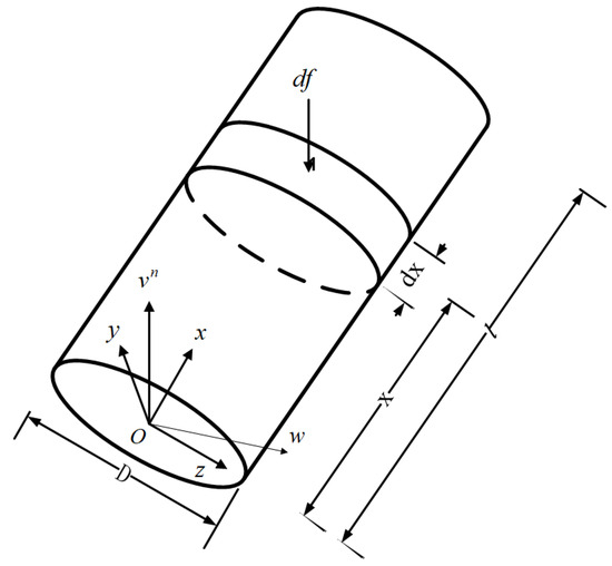
Figure 1.
The force on the cylinder as it moves through the water.
According to Morison’s empirical formula, in the coordinate system, the water resistance moment and the added mass moment are obtained:
where represents the density of water, represents the diameter of the ith cylindrical rod, represents the cross-sectional area of the ith cylindrical rod, is the velocity vector in the normal direction of the cylindrical surface, represents the water resistance coefficient, and represents the additional mass force coefficient. In the dynamic analysis of the underwater manipulator, the empirical value is often used. The values of and , which are used in this simulation, are obtained from empirical values and [4].
3. Adaptive Model Predictive Control Using Gaussian Process Regression
In this section, an adaptive MPC using GPR method is proposed and its stability is proven. To compensate for the difference between the nominal model and the actual system, GPR is used to estimate the unmodeled part of the nominal model. And the sliding window method is used to reduce the computational complexity of GPR.
3.1. Gaussian Process Regression Base on Sliding Window
In this paper, GPR is used to estimate the water resistance, added mass, buoyancy, and external disturbances mentioned above in real time. In addition, the sliding window method is adopted to select the training data, which not only satisfies the estimation accuracy, but also reduces the calculation load of the large training data set GPR.
Assume that there is a training set to be regressed. The input of the training set is X and the output is Y, the input of the test set is and the output is , and the function follows a normal distribution, that is, ∼. Without loss of generality, assume its mean value , then:
where:
and according to the conditional Gaussian distribution formula, under the condition X, Y, , follows the Gaussian distribution , namely:
According to the formula, the mean value of Gaussian process can be taken as the estimated value of :
it can be seen from Equation (9) that the prediction result of Gaussian process regression depends entirely on the mean function and covariance function. This paper considers the widely used square index (SE) kernel (Equation (10)) to calculate the covariance matrix,
where, is the signal variance of the kernel function; is a hyperparameter symmetric matrix; is the variance of noise. For convenience, all hyperparameters are described as .
After the kernel function is selected, the hyperparameters need to be optimized. The method often used is to transform the maximum a posteriori solution of the hyperparameters into the maximum marginal likelihood function solution by Bayesian theorem. First, establish the logarithmic likelihood function of the Gaussian process model [29], as shown in the Equation (11):
Then, the steepest descent method is used to solve the maximum marginal likelihood function to determine the optimal hyperparameters. Here, the partial derivative of L to is given.
In order to reduce the computational load of GPR for large training data sets, the sliding window method is used to select training data. Select sampling data before the current time k as the training set , update the hyperparameters in GPR and estimate the output corresponding to the current input . The calculation process of GPR based on sliding window is shown in Algorithm 1.
| Algorithm 1 GPR base on sliding window (, , ) |
|
3.2. Adaptive Model Predictive Control Using Gaussian Process Regression
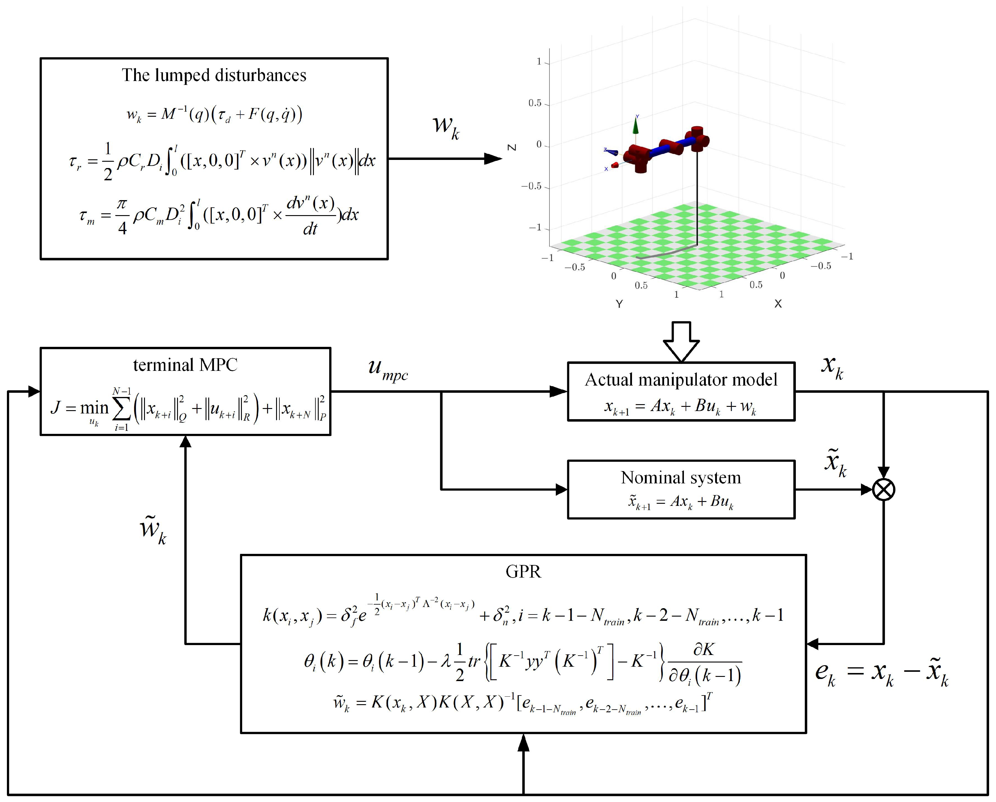
This section gives the adaptive MPC using GPR method, its structure is shown in Figure 2. Firstly, the terminal MPC controller will calculate the output torque of each joint , with the desired trajectory and status feedback value input. Then, the actual manipulator and the nominal model will be calculated at the same time, and their output is the state value and nominal state value , respectively. Finally, taking and as the input of GPR, GPR will predict the external interference value at this moment, and will be used to compensate the nominal model at the next moment. At the same time, and will be saved into the training set and the hyperparameters will be updated. The specific calculation process is as follows:

Figure 2.
Adaptive model predictive control using Gaussian process regression.
The actual system is compensated by the estimated value of unknown term and interference term through GPR. When Equation (3) is subtracted from Equation (14) to obtain , that is, the interference value at the previous time can be obtained by sampling to the actual state and the nominal state . These data will be used as hyperparameters for updating the GPR in the training set. The input of the specific GPR training set is the actual state and nominal state of the first n moments, and the output of the training set is the interference value corresponding to the time. After training GPR, input the actual state and nominal state at the current time to predict the interference value at the next time.
when , by sorting out the above formula, we can obtain:
In this way, using the estimated external interference force on the dynamic model of the underwater robotic arm in the MPC controller is equivalent to adding a feedforward correction in the control loop. While compensating for the influence of external interference force on each joint motor, it ensures the stability of the traditional terminal MPC, and during the Quadratic programming optimization process of subsequent MPC calculation, it can ensure that the output torque is always within the constraint range. Then the controlled system becomes:
where:
,
Therefore, the problem can be described as nominal terminal MPC, the cost function in a finite horizon as Equation (15)
To ensure that P is solvable, K is calculated by the infinite horizon linear quadratic regulator (LQR) of cost function J, shown as (17)
where:
Then, the first term of the optimal solution sequence of the optimization problem is the closed-loop control quantity, shown as (18). The calculation process of the adaptive MPC using GPR method is shown in Algorithm 2.
Here, we can propose:
Theorem 1.
If the constrained optimization problem (15) has a solution at the initial time, then it has a solution at any time greater than 0, and the closed-loop system is asymptotically stable.
Proof.
Assume that a group of optimal control sequences with prediction interval N at time k are:
The corresponding set of optimal state sequences and loss functions are:
select closed-loop controller as then the status at time is
select a group of control sequences at time as
then the corresponding status sequence is:
□
| Algorithm 2 The adaptive MPC using GPR method (J,) |
|
Then the corresponding loss function is shown in Equation (20), since Q and R are both positive definite, , we can see that is a closed-loop system Lyapunov function, and it is monotonically decreasing, and the system is asymptotically stable.
In summary, the sliding-window Gaussian process regression can utilize both actual and nominal state variables during the underwater manipulator’s operation to estimate real-time external disturbances such as fluid forces and unknown resistances that the manipulator will experience in future time steps. The estimated external disturbances are then used to compensate for the effects on joint torques in the output torque of MPC. This enables the underwater manipulator to adaptively adjust and compensate for various fluid-induced forces without manually readjusting parameters in the underwater environment, thereby enhancing the robustness of the controller and improving the adaptability of the underwater manipulator to its surroundings.
4. Simulation Results
In this paper, the trajectory tracking problem of the six-degrees-of-freedom manipulator is used to verify the effectiveness of the adaptive MPC using GPR method. In this section, the effectiveness of GPR for real-time estimation of the hydrodynamic term and time-varying external interference is analyzed. In addition, the trajectory tracking control effect of the adaptive MPC using GPR method under the complete dynamic model of the underwater six-degrees-of-freedom manipulator is given.
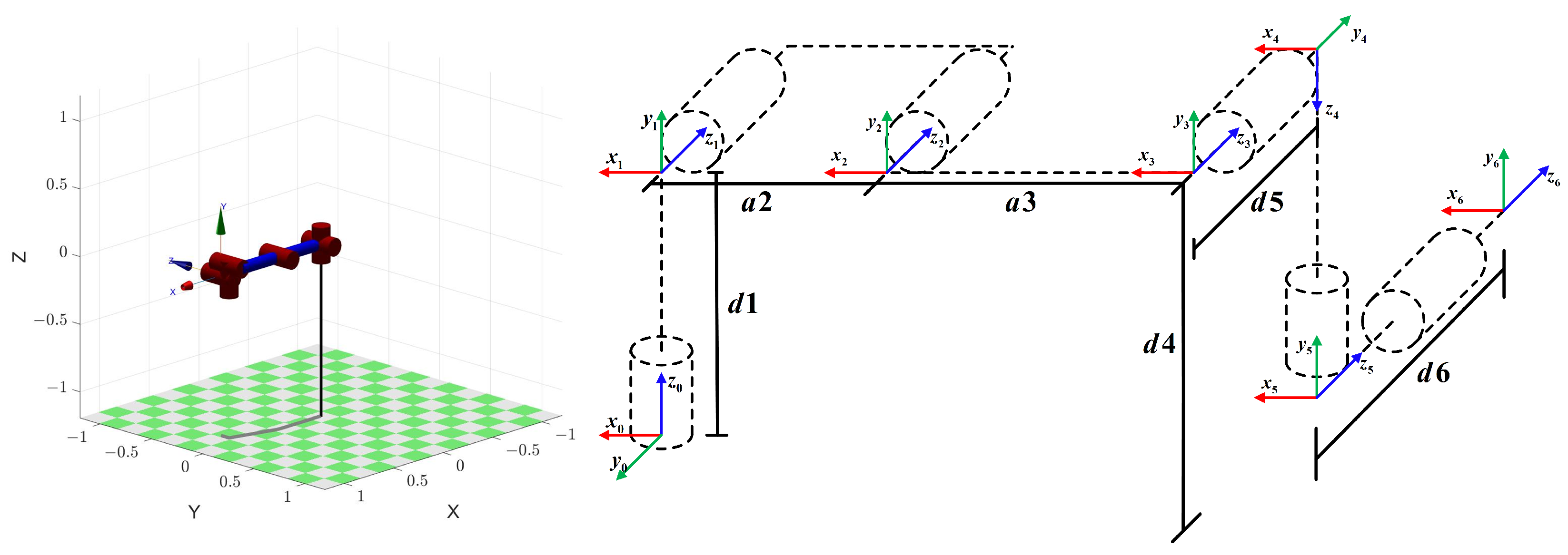
The structure diagram of the 6-DOF manipulator is shown in Figure 3. The first joint of the manipulator will be fixed on a fixed platform. The specific kinematics and dynamics parameters are shown in Table A1 and Table A2 in Appendix A. The parameter of manipulators are derived from UR5, which is a product manufactured by universal robots [30]. The parameter equations of the hydrodynamic model based on the underwater manipulator are described in Appendix B. The codes run in the computer with an Intel (R) Core (TM) i7-12700F CPU @ 2.1 GHz 16 GB RAM. The simulation experiment in this manuscript is run in matlabR2021a, and the differential equation is calculated using the fourth-order Runge–Kutta method (ode45). The simulation task is to complete the trajectory tracking of the manipulator, the desired joint trajectory is shown as (21), and the working disturbance is given by (22); here, the trigonometric functions varying in a certain range is used to express the influence of unknown ocean currents on the joints of the underwater manipulator, which will be added to the joint velocity term in the actual state value. Moreover, the influence of measurement noise on the control performance is considered, Gaussian white noise with a mean of 0 and a variance of 0.001 is taken as the measurement noise and added to the output state variable at each simulation cycle.
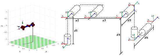
Figure 3.
6-DOF manipulator.
The parameters of the adaptive MPC using GPR method are selected as follows. Firstly, the initialization process of GPR is described in Section 3.1, the initial value of hyperparameters is set as , the size of the sliding window is selected to 10. Secondly, for the parameters of the MPC cost function, the terminal penalty matrix P, the infinite horizon LQP control gain K, and the terminal area will be determined according to the steps described in Section 3.2. Here, the control parameters are selected as , , , and .
4.1. The Simulation of Gaussian Process Regression
The external interference is considered as the sum of water resistance, added mass, buoyancy and ocean current interference. The Gaussian process regression of sliding window is used to predict the external interference in real time and compensate for the unmodeled part of the nominal dynamic model.
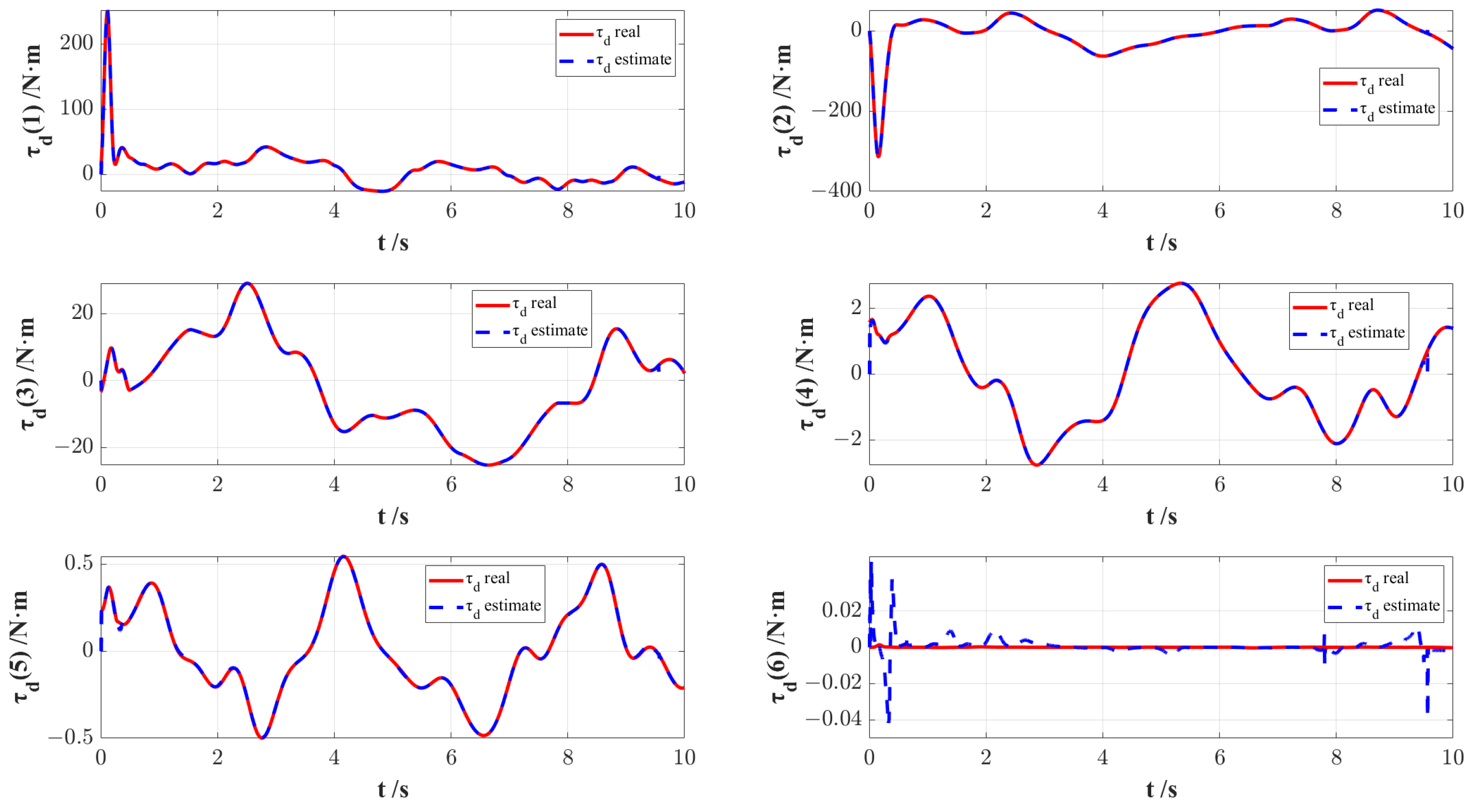
The actual external interference and the predicted external interference through GPR based on sliding window are shown in Figure 4; it can be seen that external interferences have a great impact on joint torque, especially for the first joint and the second joint, as both exceed 200 at the beginning of the simulation. In addition, the external interference is strongly nonlinear with time, which has a great impact on the prediction performance and control performance.
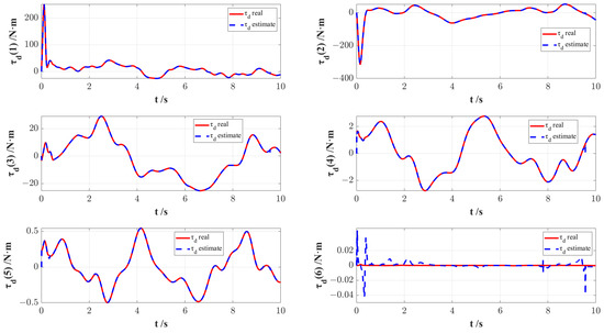
Figure 4.
The real value and estimated value of external interference.
The external interference force on each joint mainly comes from the water resistance and added mass force caused by the upstream surface of the connecting rod during the movement of the manipulator. The first and second joints are located at the base, and the interference force received by each connecting rod will be transmitted to the motor of these two joints. The vertical force will be superimposed on the first joint, and the horizontal force will be superimposed on the second joint, so the first two joints will receive the maximum external interference force. Similarly, it can be concluded that the joint motor closer to the end of the robotic arm is subjected to less interference force, and the simulation results are also consistent with the actual situation, indicating the correctness of the established dynamic model of the underwater robotic arm.
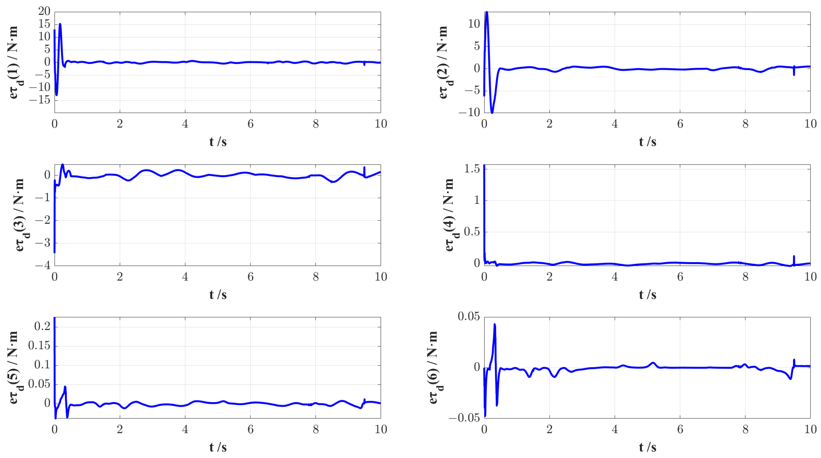
However, the predicted value can well track the real value, the change of prediction error with time is shown in Figure 5. The predicted value can converge to the actual value within 1 s, and the error of six joints are always controlled within 0.1 . After the convergence of the estimated value, the error between the estimated value and the real value fluctuates in a small range, because the Gradient descent used by GPR in the hyperparameter optimization may not find the optimal value in a limited number of steps, but does not affect the accuracy of the estimation. The estimation error has been kept within the acceptable accuracy range.
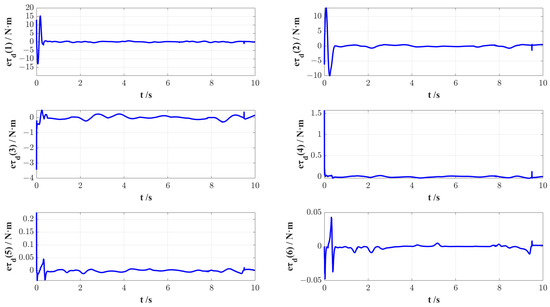
Figure 5.
Difference between real value and estimated value of external interference.
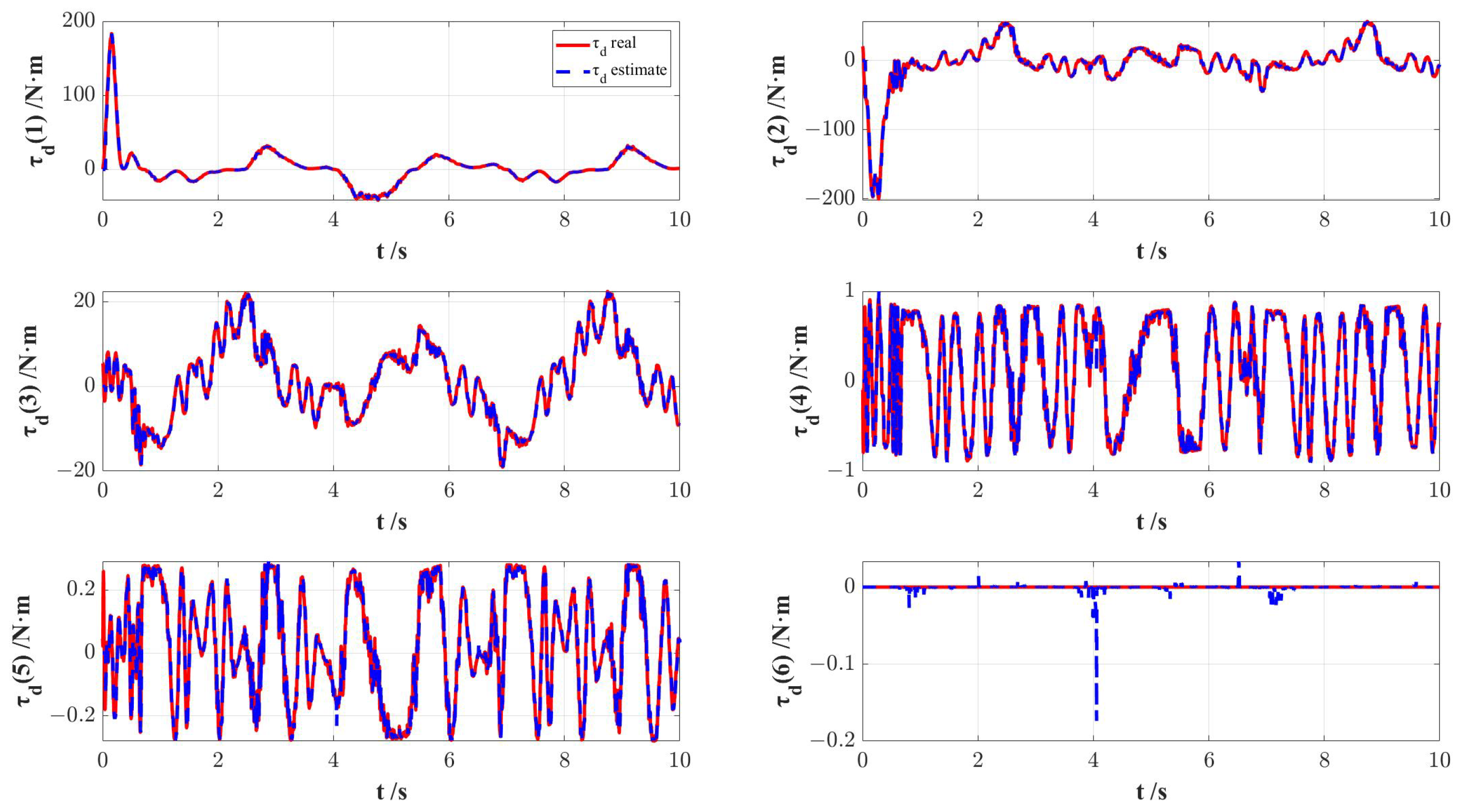
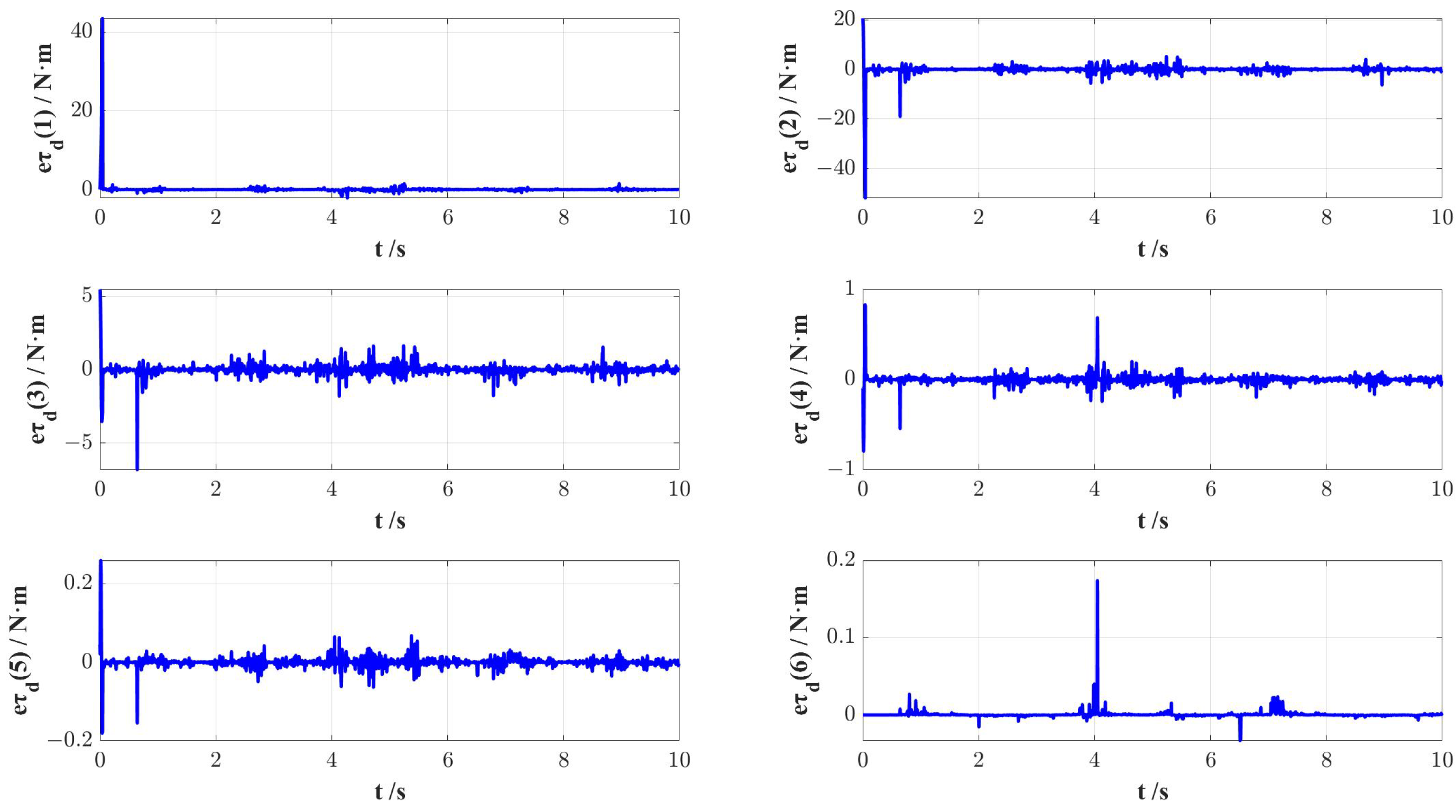
After the measurement noises are introduced, the actual value and the estimated value of external interference are shown in Figure 6, the estimation of interference will jitter in a small range near the true value. However, it can be seen from Figure 7 that the estimation error is still within a acceptable range, and it is still effective for the interference compensation of the controller.
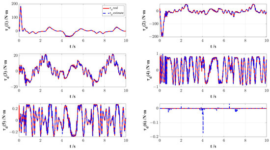
Figure 6.
The real value and estimated value of external interference with measurement noises.
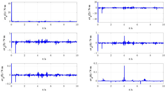
Figure 7.
Difference between real value and estimated value of external interference with measurement noises.
4.2. The Simulation of Adaptive Model Predictive Control Using Gaussian Process Regression
In this section, we take the trajectory tracking of 6-DOF underwater manipulator as the task, and verify the effectiveness of proposed control method by displaying its position-tracking curve, speed-tracking curve, and output torque curve. Compared with the traditional MPC and sliding mode control methods, the simulation results show that the proposed control method has better control accuracy.
In the simulation experiment in this paper, the initial state of the simulation object, the six-degrees-of-freedom underwater manipulator, is that the angular positions of the six joints are all at 0 rad, and the angular velocities of the six joints are also at 0 rad/s. Each joint of the underwater manipulator starts to track the desired trajectory expressed in Equation (21) at the initial time. The six expected trajectories are linear combinations of each Trigonometric functions, and the set trajectory curve position, speed and acceleration terms are continuously derivable. Under the condition that the articulated motor can be completed and the six manipulators move at the same time, the forces between the articulated motors interfere with each other, fully verifying the control performance of the underwater manipulator. And in the underwater environment, the motion speed and acceleration of the connecting rod are proportional to the fluid resistance and added mass force suffered by the joint. The trajectory curve of the joint motor with high motion speed will also increase the fluid resistance and added mass force suffered by the underwater manipulator, which is also a challenge to the controller designed in this paper.
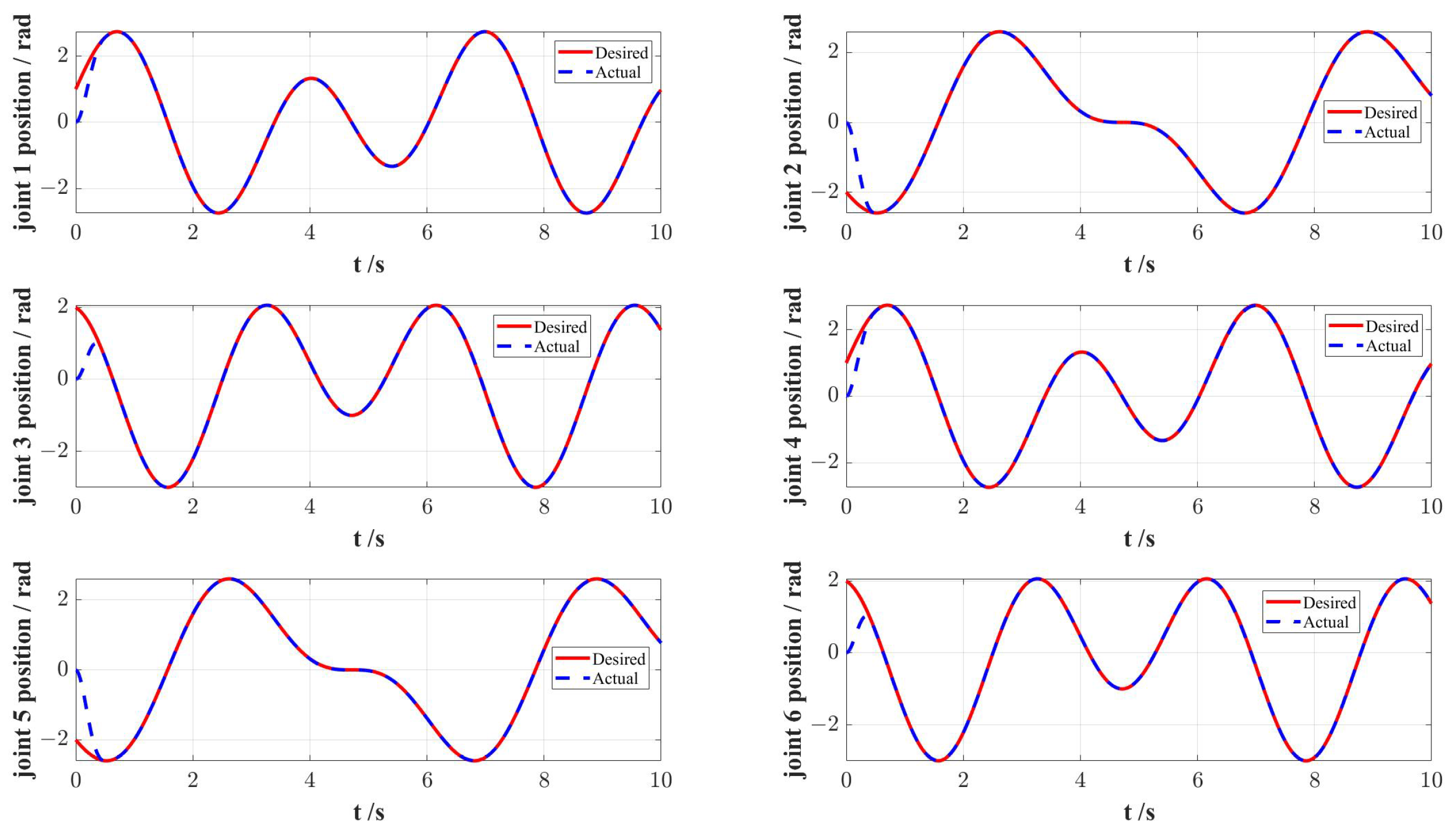
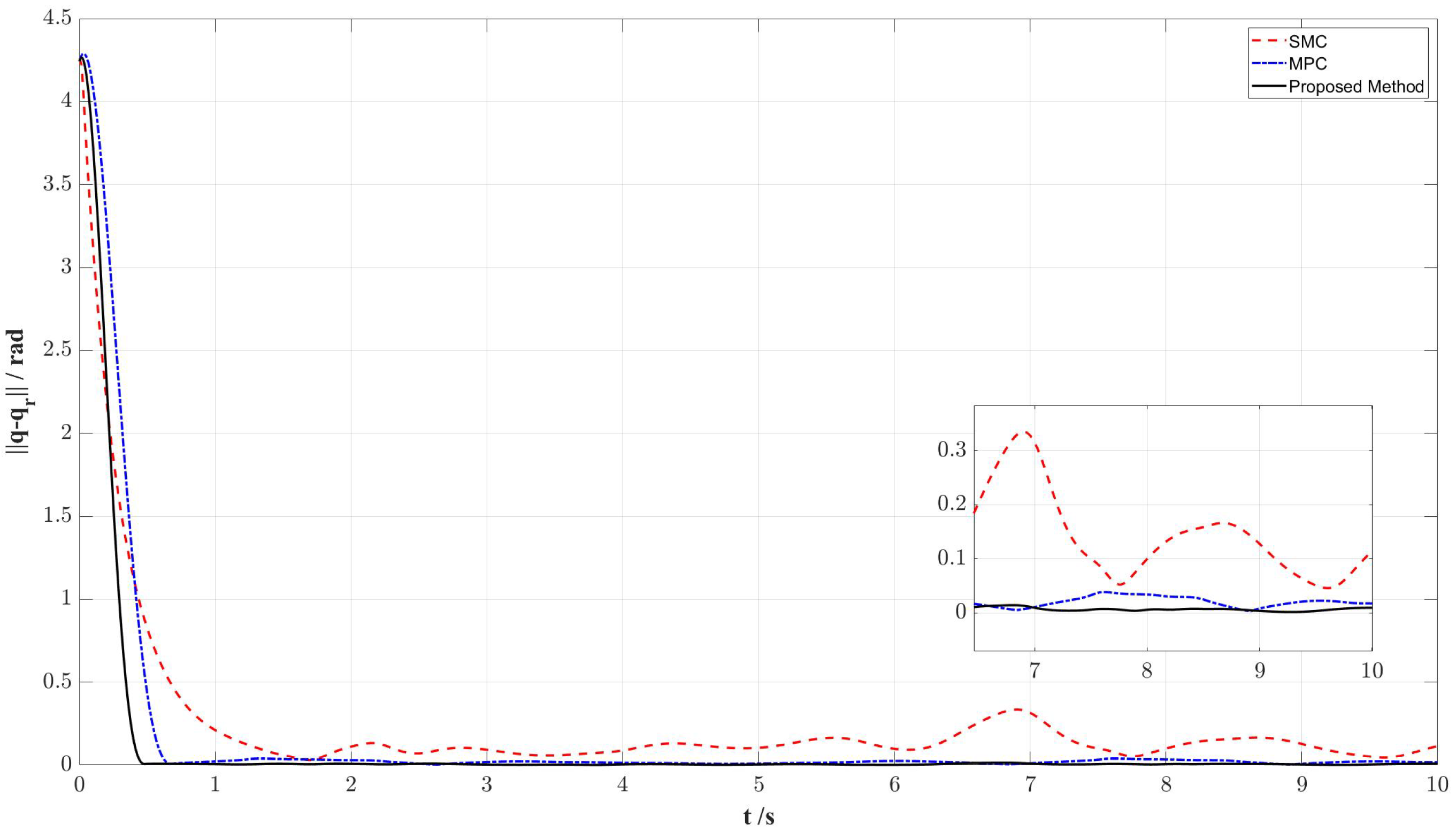
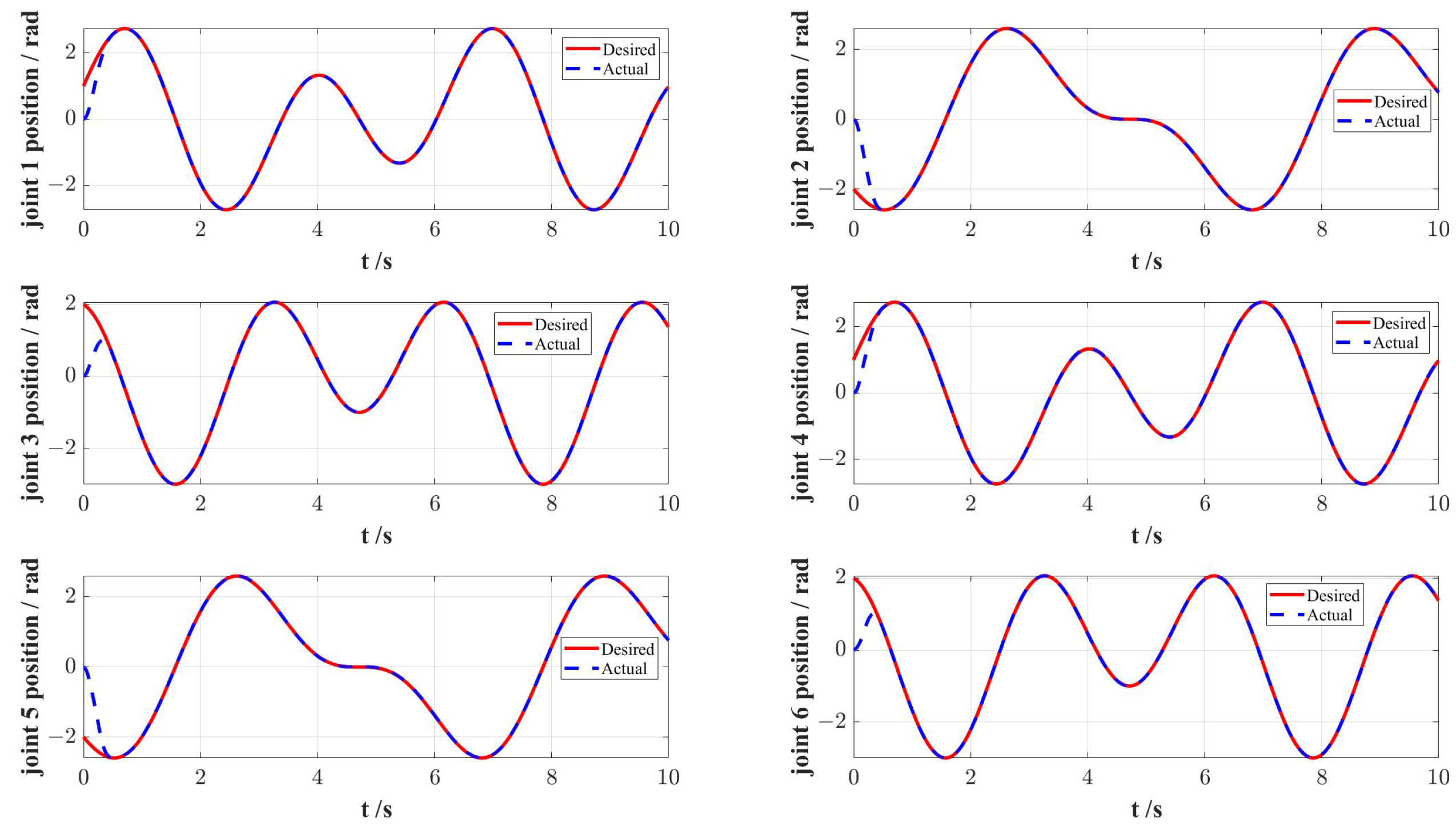
The desired joint position track and the actual simulated joint position track are shown in Figure 8. It can be seen that the actual value can well track the desired value. The actual value can keep up with the desired value within 1 s, and the error is always controlled within a small range, the two-norm of error is shown in Figure 9. The figure also shows the error of traditional MPC and sliding mode control, and it can be seen that the control effect of the proposed method is obviously superior to both in terms of rate of convergence and steady-state error. The mean square error of each joint is shown in Table 1.
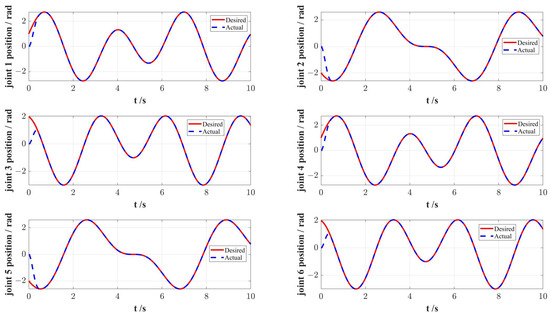
Figure 8.
Position tracking performance by manipulator joints.
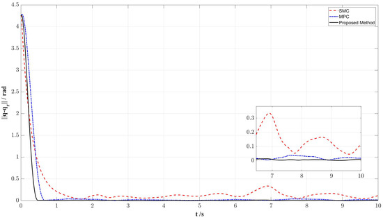
Figure 9.
The comparison of tracking error by manipulator joints.

Table 1.
Trajectory tracking errors in three controllers.
The position control accuracies of joint 1 to joint 6 were increased by 44.85%, 7.68%, 25.87%, 55.97%, 41.16%, and 28.79%, respectively, and the average control accuracy was increased by 34.05%.
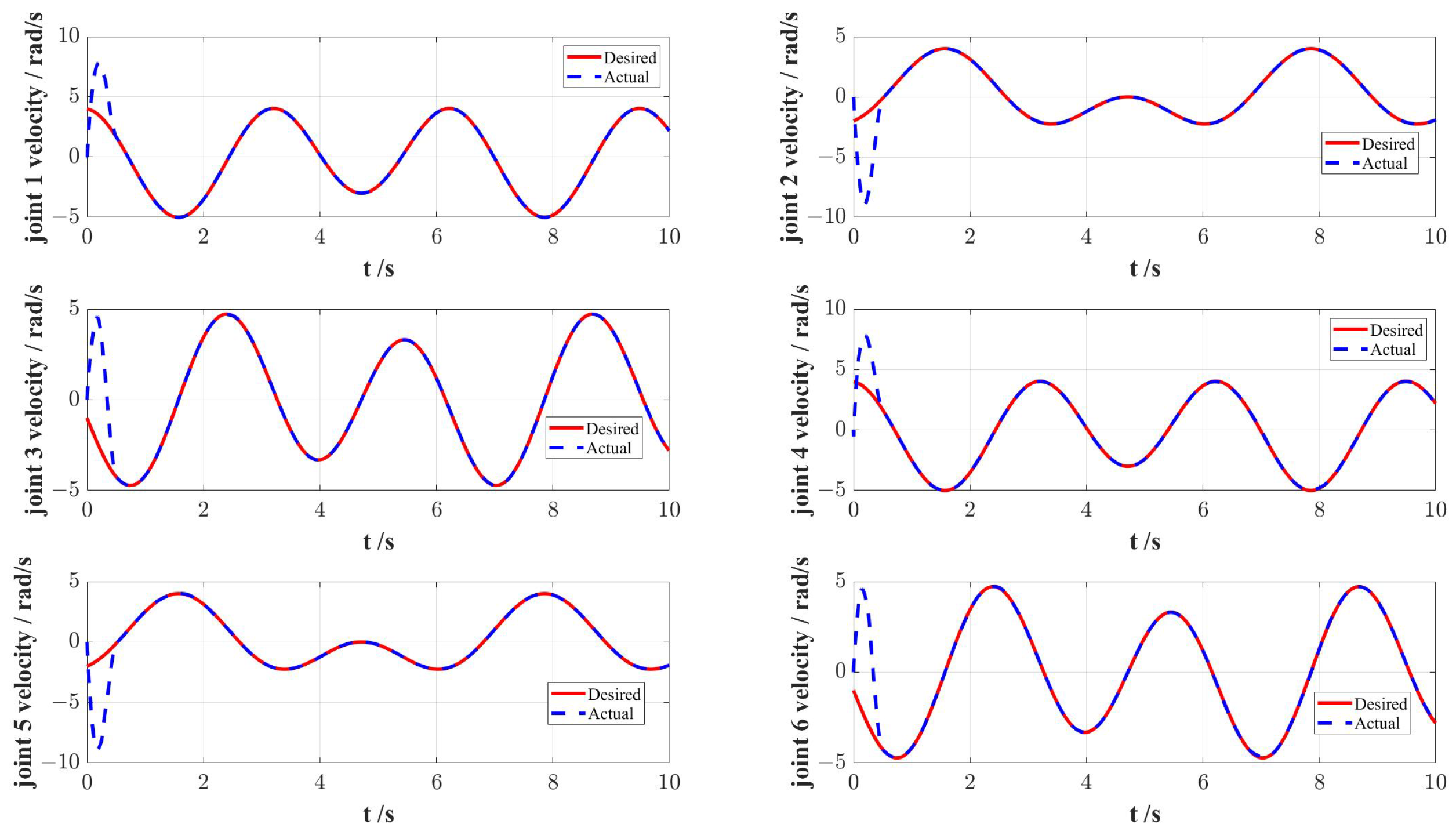
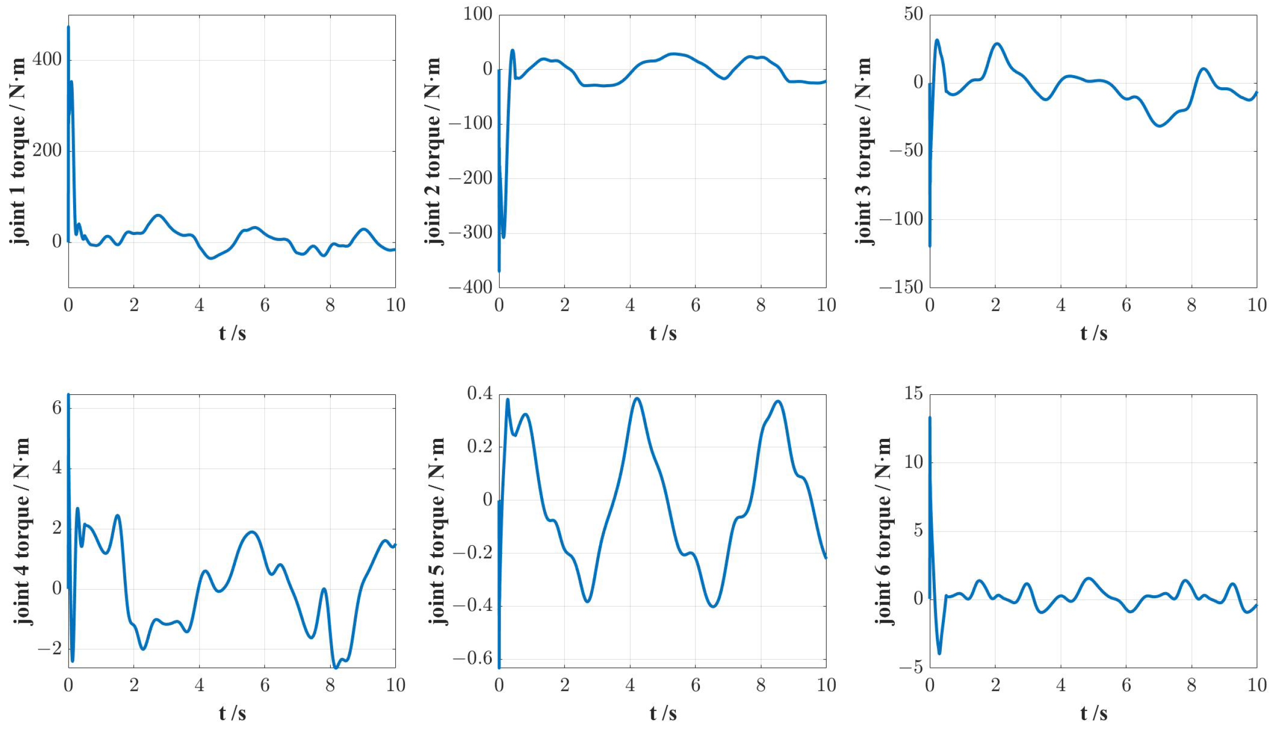
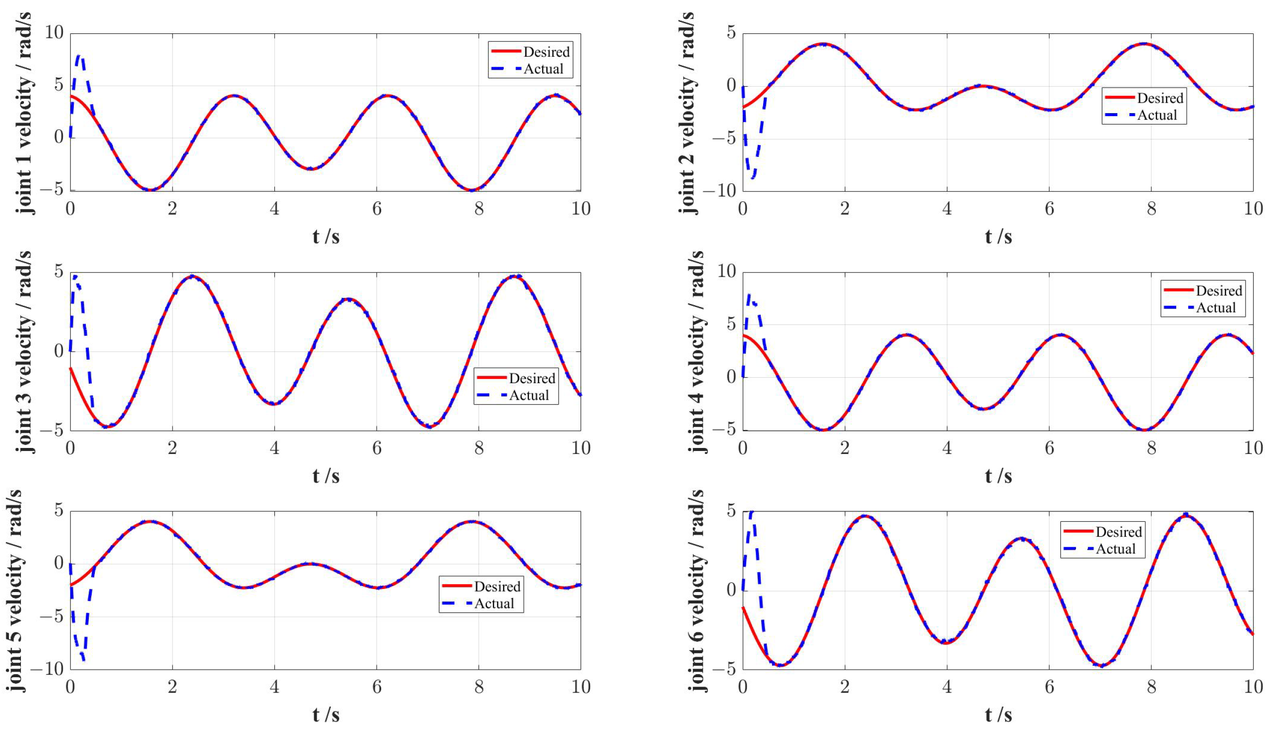
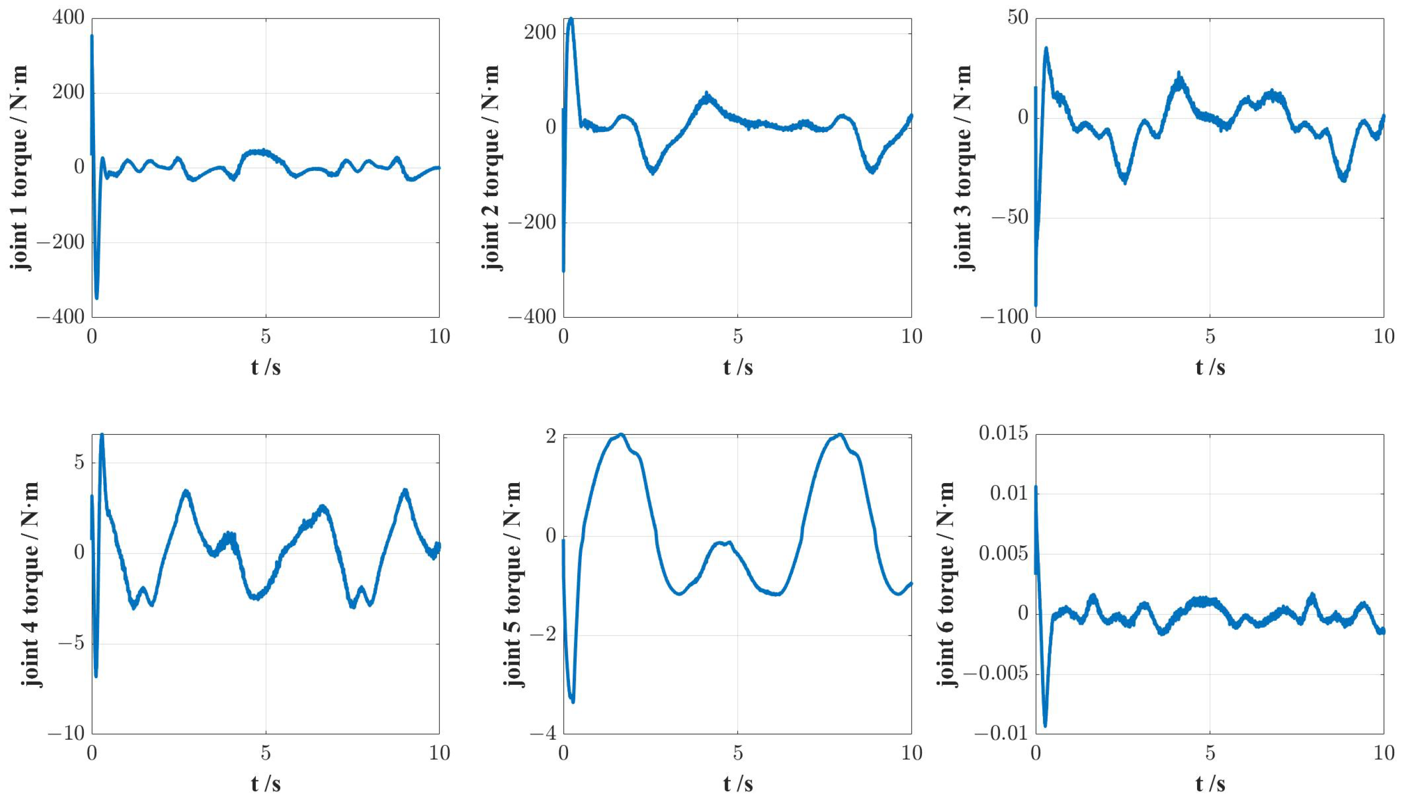
The desired joint speed track and the actual simulated joint speed track are shown in Figure 10, and the speed following effect is also good. At the same time, the joint torque change curve is shown in Figure 11. The torque changes smoothly without obvious jitter, and the output torque of each joint is within the constraint range. Compared with Figure 4, a large part of the output torque is overcoming external interference during the movement, which also shows the good robustness of the adaptive MPC using GPR method.
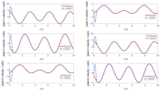
Figure 10.
Velocity tracking performance by manipulator joints.
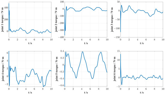
Figure 11.
Output torque by manipulator joints.
The Gaussian white noises with mean 0 and variance 0.001 are introduced into the feedback values of joint position and joint velocity, and the obtained results are presented in Figure 12, Figure 13 and Figure 14.
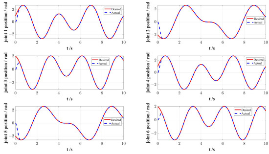
Figure 12.
Position tracking performance by manipulator joints with measurement noises.
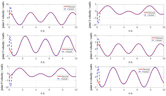
Figure 13.
Velocity tracking performance by manipulator joints with measurement noises.
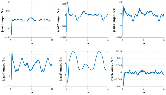
Figure 14.
Output torque by manipulator joints with measurement noises.
When the measurement noise is considered in the simulation experiment, the desired joint position and the actual joint position as shown in Figure 12 still maintains a fast and stable tracking desired trajectory. The desired joint speed and the actual simulated joint speed as given in Figure 13, although the actual joint speed contains a small vibration, it can track the desired joint speed and is stable in the overall tracking process. Meanwhile, the actual output torque as shown in Figure 14 is relatively stable and there is no large vibration.
Figure 15 shows the trajectory-tracking errors of each joint of the underwater manipulator when there are measurement noises. It can be seen that the position control accuracy of the proposed control method is still better than the SMC method and the traditional MPC method. The mean square error of each joint is shown in Table 2.
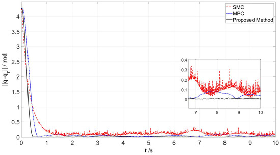
Figure 15.
The comparison of tracking error by manipulator joints with measurement noises.
Table 2.
Trajectory-tracking errors in three controllers with measurement noises.
Compared with SMC, the proposed method has improved the control accuracy. Compared with MPC, the proposed method also has a certain improvement in control accuracy, the position control accuracy of joint 1 to joint 6 are increased by 38.58%, 36.28%, 60.95%, 45.95%, 91.55%, and 40.31%, respectively, and the average control accuracy is increased by 52.27%. Compared with the results presented in Table 1, this increase is even more significant when the measurement noises are taken into account.
5. Conclusions
In this paper, the Lagrange equation and Morrison formula are combined to establish an accurate dynamic model of the 6-DOF underwater manipulator in a still-water environment. An improved MPC method is proposed to embed the GPR algorithm into the accurate trajectory tracking control of underwater manipulator. GPR was used to predict water resistance, added mass, buoyancy, and external disturbances in real time, and to compensate for the unmodeled part of the nominal dynamic model. MPC realizes the accurate calculation of the dynamic model. Some numerical experiments and simulation results fully demonstrate the effectiveness and efficiency of the adaptive MPC using GPR method. In future research, the control performance of the proposed method will be further verified in actual underwater environments and on actual underwater manipulators.
Author Contributions
Conceptualization and methodology, J.X., W.L. and L.L.; Testing setpub, J.X. and L.L.; Testing conduction and data analysis, J.X. and W.L.; Writing—original draft preparation, all authors; Writing—review and editing, all authors; Funding acquisition, W.L. All authors have read and agreed to the published version of the manuscript.
Funding
This work is supported in part by the National Science Foundation of China (Project No. 61903304), in part by the National Key Research and Development Program of China (Project No. 2016YFC0301700), in part by the Fundamental Research Funds for the Central Universities (Project No. 3102020HHZY030010), In part by Science and Technology Program of Xi’an (Project No. 2020KJRC0119), and in part by the 111 Project under grant No. B18041.
Institutional Review Board Statement
Not applicable.
Informed Consent Statement
Not applicable.
Data Availability Statement
The data presented in this study are available by sending a request to 2018260584@mail.nwpu.edu.cn.
Conflicts of Interest
The authors declare no conflict of interest.
Abbreviations
The following abbreviations are used in this manuscript:
| MPC | Model predictive control |
| GPR | Gaussian process regression |
| SMC | Sliding mode control |
| ESO | Extened state observer |
| GP | Gaussian processes |
| DOF | Degree of freedom |
| PID | proportional–integral–derivative |
| EKF | Extended Kalman Filter |
| RBFNNs | radial basis function neural networks |
Appendix A
Table A1.
The D-H parameter of the manipulator.
Table A1.
The D-H parameter of the manipulator.
| Link | Dryweight (kg) | Buoyancy (kg) | |||||
|---|---|---|---|---|---|---|---|
| 0 | 90 | 0.089459 | 0.083 | 3.7 | 0.484 | ||
| −0.425 | 0 | 0 | 0.083 | 9.393 | 2.2995 | ||
| −0.39225 | 0 | 0 | 0.0745 | 2.33 | 1.7099 | ||
| 0 | 90 | 0.10915 | 0.010915 | 1.1219 | 0.0102 | ||
| 0 | −90 | 0.09465 | 0.075 | 1.1219 | 0.4182 | ||
| 0 | 0 | 0.0823 | 0.075 | 0.1897 | 0.3636 |
Table A2.
The Inertia (g·m) and center () of gravity of the manipulator.
Table A2.
The Inertia (g·m) and center () of gravity of the manipulator.
| Link | ||||||
|---|---|---|---|---|---|---|
| 3.75 | 7.65 | 7.65 | 0 | −2.561 | 0.193 | |
| 8.5 | 208 | 208 | 21.25 | 0 | 11.34 | |
| 0.246 | 7.19 | 7.19 | 15 | 0 | 2.65 | |
| 0.909 | 1.19 | 1.19 | 0 | −0.18 | 1.634 | |
| 0.909 | 1.19 | 1.19 | 0 | −0.18 | 1.634 | |
| 0.122 | 0.0821 | 0.0821 | 0 | 0 | 0.1159 |
The center of gravity of each link is relative to the link center. The link is placed horizontally, with the Y-axis pointing to the right in the axial direction of the link, the Z-axis pointing straight down, and the X-axis following the right-hand rule pointing in the radial direction of the link.
Appendix B
Appendix B.1. Water Resistance Torque Tr = [Tr1, Tr2, Tr3, Tr4, Tr5]
- The water resistance torque on the first joint :where:
- The water resistance torque on the first joint :where:
- The water resistance torque on the first joint :
- The water resistance torque on the first joint :
- The water resistance torque on the first joint :
Appendix B.2. Additional Mass Torque Tm = [Tm1, Tm2, Tm3, Tm4, Tm5]
- The additional mass torque on the first joint :where:
- The additional mass torque on the first joint :where:
- The additional mass torque on the first joint :
- The additional mass torque on the first joint :
- The additional mass torque on the first joint :
References
- Sivcev, S.; Coleman, J.; Omerdic, E.; Dooly, G.; Toal, D. Underwater manipulators: A review. Ocean Eng. 2018, 163, 431–450. [Google Scholar] [CrossRef]
- Zhang, Q.; Chen, J.; Huo, L.; Kong, F.; Du, L.; Cui, S.; Zhao, Y.; Tang, Y. 7000M pressure experiment of a dep-sea hydraulic manipulator system. In Proceedings of the 2014 OCEANS-St. John’s, St. John’s, NL, Canada, 14–19 September 2014; pp. 1–5. [Google Scholar]
- Marani, G.; Choi, S.K.; Yuh, J. Underwater autonomous manipulation for intervention missions AUVs. Ocean Eng. 2009, 36, 15–23. [Google Scholar] [CrossRef]
- Yuguang, Z.; Fan, Y. Dynamic modeling and adaptive fuzzy sliding mode control for multi-link underwater manipulators. Ocean Eng. 2019, 187, 106202. [Google Scholar] [CrossRef]
- Zhou, S.; Shen, C.; Xia, Y.; Chen, Z.; Zhu, S. Adaptive robust control design for underwater multi-DoF hydraulic manipulator. Ocean Eng. 2022, 248, 110822. [Google Scholar] [CrossRef]
- Han, L.; Tang, G.; Cheng, M.; Huang, H.; Xie, D. Adaptive Nonsingular Fast Terminal Sliding Mode Tracking Control for an Underwater Vehicle-Manipulator System with Extended State Observer. J. Mar. Sci. Eng. 2021, 9, 501. [Google Scholar] [CrossRef]
- Shang, D.; Li, X.; Yin, M.; Li, F. Vibration suppression method for flexible link underwater manipulator considering torsional flexibility based on adaptive PI controller with nonlinear disturbance observer. Ocean Eng. 2023, 274, 114111. [Google Scholar] [CrossRef]
- Cai, M.; Wang, Y.; Wang, S.; Wang, R.; Ren, Y.; Tan, M. Grasping Marine Products With Hybrid-Driven Underwater Vehicle-Manipulator System. IEEE Trans. Autom. Sci. Eng. 2020, 17, 1443–1454. [Google Scholar] [CrossRef]
- Shang, D.; Li, X.; Yin, M.; Zhou, S. Rotation tracking control strategy of underwater flexible telescopic manipulator based on neural network compensation for water environment disturbance. Ocean Eng. 2023, 284, 115245. [Google Scholar] [CrossRef]
- Filaretov, V.F.; Konoplin, A.Y.; Zuev, A.V.; Krasavin, N.A. A method to synthesize high-precision motion control systems for underwater manipulator. Int. J. Simul. Model. 2021, 20, 625–636. [Google Scholar] [CrossRef]
- Lv, J.Q.; Wang, Y.; Tang, C.; Wang, S.; Xu, W.X.; Wang, R. Disturbance Rejection Control for Underwater Free-Floating Manipulation. IEEE/ASME Trans. Mechatronics 2021, 27, 3742–3750. [Google Scholar] [CrossRef]
- Zhang, M.; Song, G.; Mao, J.; Wang, F.; Zhou, J. Chattering suppression and hydrodynamic disturbance estimation of underwater manipulators using adaptive fuzzy sliding mode control. Trans. Inst. Meas. Control 2023, 1, 1–12. [Google Scholar] [CrossRef]
- Zhou, Z.; Tang, G.; Xu, R.; Han, L.; Cheng, M. A Novel Continuous Nonsingular Finite–Time Control for Underwater Robot Manipulators. J. Mar. Sci. Eng. 2021, 9, 269. [Google Scholar] [CrossRef]
- Yu, X.B.; He, W.; Li, H.Y.; Sun, J. Adaptive Fuzzy Full-State and Output-Feedback Control for Uncertain Robots With Output Constraint. IEEE Trans. Syst. Man Cybern. Syst. 2021, 51, 6994–7007. [Google Scholar] [CrossRef]
- Mayne, D.Q. Model predictive control: Recent developments and future promise. Automatica 2014, 50, 2967–2986. [Google Scholar] [CrossRef]
- Dai, Y.; Yu, S.; Yan, Y. An Adaptive EKF-FMPC for the Trajectory Tracking of UVMS. IEEE J. Ocean. Eng. 2020, 45, 699–713. [Google Scholar] [CrossRef]
- Dai, Y.; Gao, H.W.; Yu, S.H.; Ju, Z.J. A fast tube model predictive control scheme based on sliding mode control for underwater vehicle-manipulator system. Ocean Eng. 2022, 254, 111259. [Google Scholar] [CrossRef]
- Kang, E.; Qiao, H.; Gao, J.; Yang, W. Neural network-based model predictive tracking control of an uncertain robotic manipulator with input constraints. ISA Trans. 2021, 109, 89–101. [Google Scholar] [CrossRef]
- Yang, H.; Liu, J.; Fang, X.; Chen, X.; Gong, Z.; Wang, S. Prediction model-based learning adaptive control for underwater grasping of a soft manipulator. Int. J. Intell. Robot. Appl. 2021, 5, 337–353. [Google Scholar] [CrossRef]
- Chen, S.W.; Wang, T.Y.; Atanasov, N.; Kumar, V.; Morari, M. Large scale model predictive control with neural networks and primal active sets. Automatica 2022, 135, 109947. [Google Scholar] [CrossRef]
- Carlucho, I.; Stephens, D.W.; Barbalata, C. An adaptive data-driven controller for underwater manipulators with variable payload. Appl. Ocean. Res. 2021, 113, 102726. [Google Scholar] [CrossRef]
- Yang, L.; Wang, K.; Mihaylova, L. Online Sparse Multi-Output Gaussian Process Regression and Learning. IEEE Trans. Signal Inf. Process. Over Netw. 2019, 5, 258–272. [Google Scholar] [CrossRef]
- Gijsberts, A.; Metta, G. Real-time model learning using Incremental Sparse Spectrum Gaussian Process Regression. Neural Netw. 2013, 41, 59–69. [Google Scholar] [CrossRef] [PubMed]
- Schürch, M.; Azzimonti, D.; Benavoli, A.; Zaffalon, M. Recursive estimation for sparse Gaussian process regression. Automatica 2020, 120, 109127. [Google Scholar] [CrossRef]
- Hewing, L.; Kabzan, J.; Zeilinger, M.N. Cautious Model Predictive Control Using Gaussian Process Regression. IEEE Trans. Control Syst. Technol. 2020, 28, 2736–2743. [Google Scholar] [CrossRef]
- Janssen, N.H.J.; Kools, L.; Antunes, D.J. Embedded Learning-based Model Predictive Control for Mobile Robots using Gaussian Process Regression. In Proceedings of the 2020 American Control Conference (ACC), Denver, CO, USA, 1–3 July 2020; pp. 1124–1130. [Google Scholar]
- Siciliano, B.; Sciavicco, L.; Villani, L.; Oriolo, G. Robotics Modelling, Planning and Control; Springer: Berlin/Heidelberg, Germany, 2008. [Google Scholar]
- Sharma, A.K.; Saha, S.K. Simplified Drag Modeling for the Dynamics of an Underwater Manipulator. IEEE J. Ocean. Eng. 2021, 46, 40–55. [Google Scholar] [CrossRef]
- Liu, H.; Ong, Y.-S.; Shen, X.; Cai, J. When Gaussian Process Meets Big Data: A Review of Scalable GPs. IEEE Trans. Neural Netw. Learn. Syst. 2020, 31, 4405–4423. [Google Scholar] [CrossRef]
- U. Robots. UR5 Technical Specifications. 2016. Available online: http://www.universal-robots.com/products/ur5-robot/ (accessed on 2 June 2023).


Disclaimer/Publisher’s Note: The statements, opinions and data contained in all publications are solely those of the individual author(s) and contributor(s) and not of MDPI and/or the editor(s). MDPI and/or the editor(s) disclaim responsibility for any injury to people or property resulting from any ideas, methods, instructions or products referred to in the content. |
© 2023 by the authors. Licensee MDPI, Basel, Switzerland. This article is an open access article distributed under the terms and conditions of the Creative Commons Attribution (CC BY) license (https://creativecommons.org/licenses/by/4.0/).