
Computational Analysis for Estimation of Mooring Force Acting on Various Ships in Busan New Port
Abstract
:1. Introduction
2. Numerical Setup
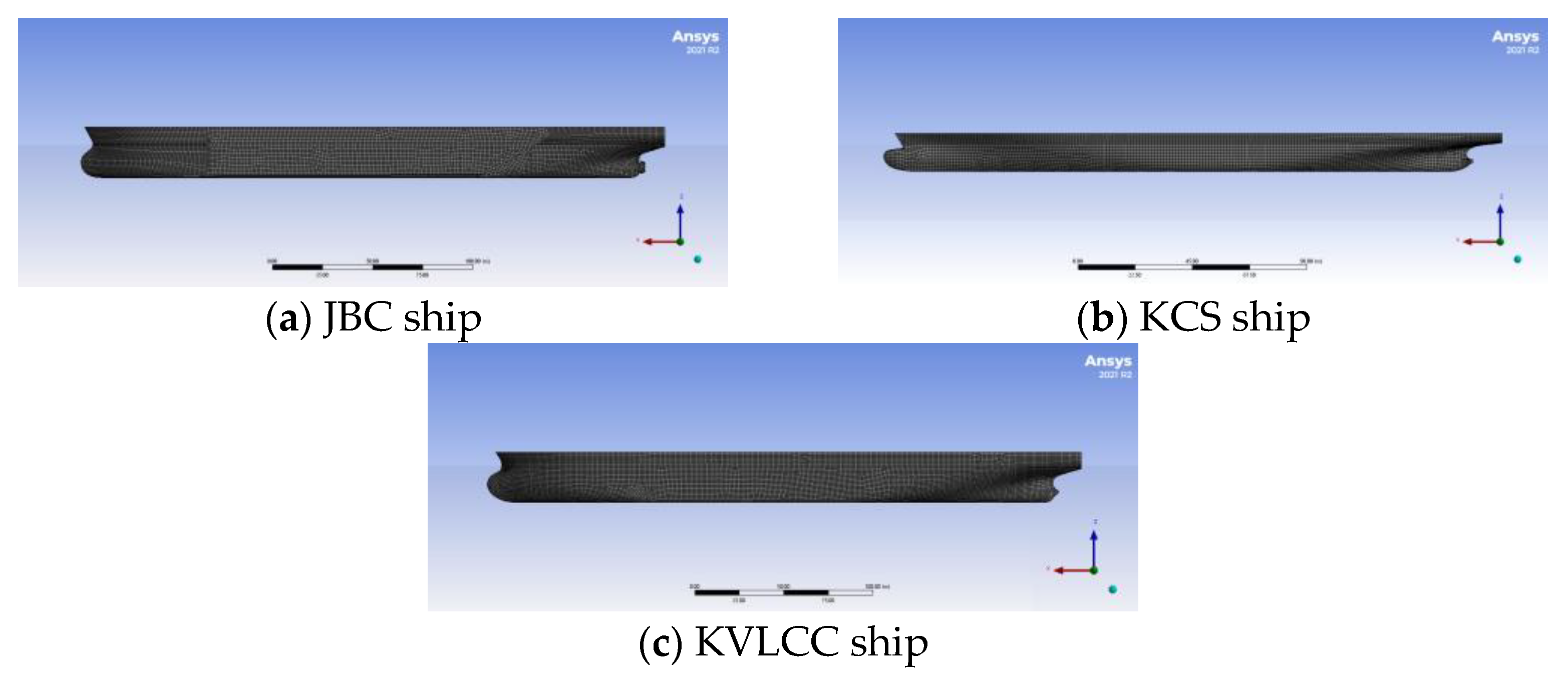
2.1. Target Ship
2.2. Ocean Environmental Condition
2.3. Governing Equation for Simulations
2.3.1. Viscous Fluid Solver
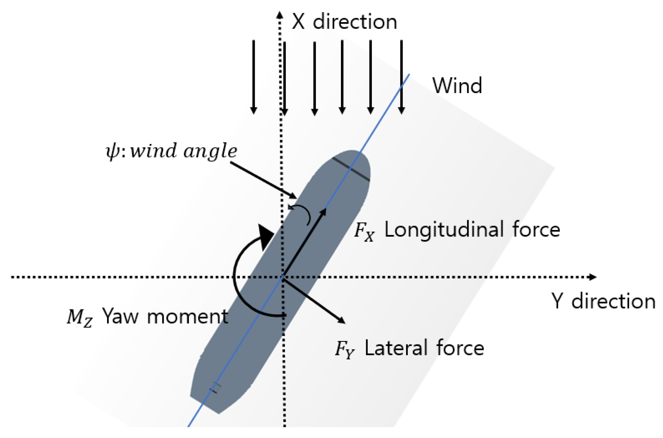
2.3.2. Calculation of the Current Force
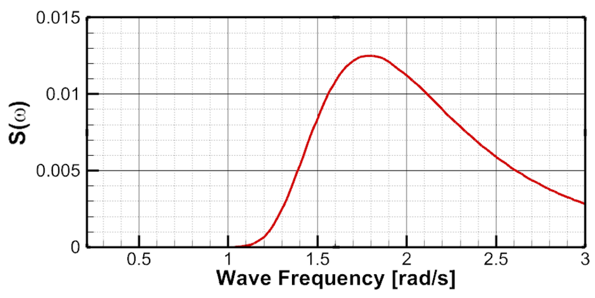
2.3.3. Calculation of the Wave Force
3. Numerical Results
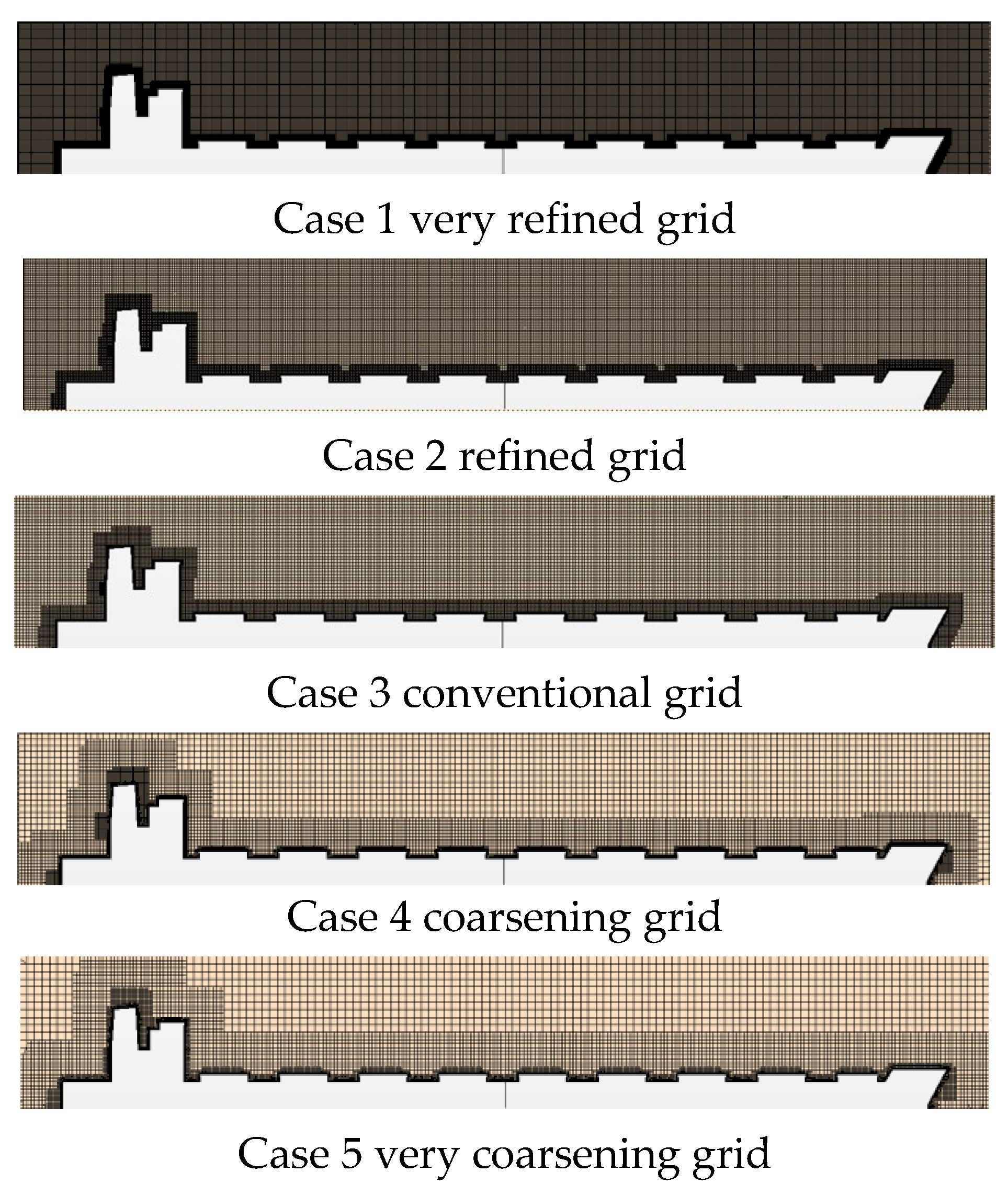
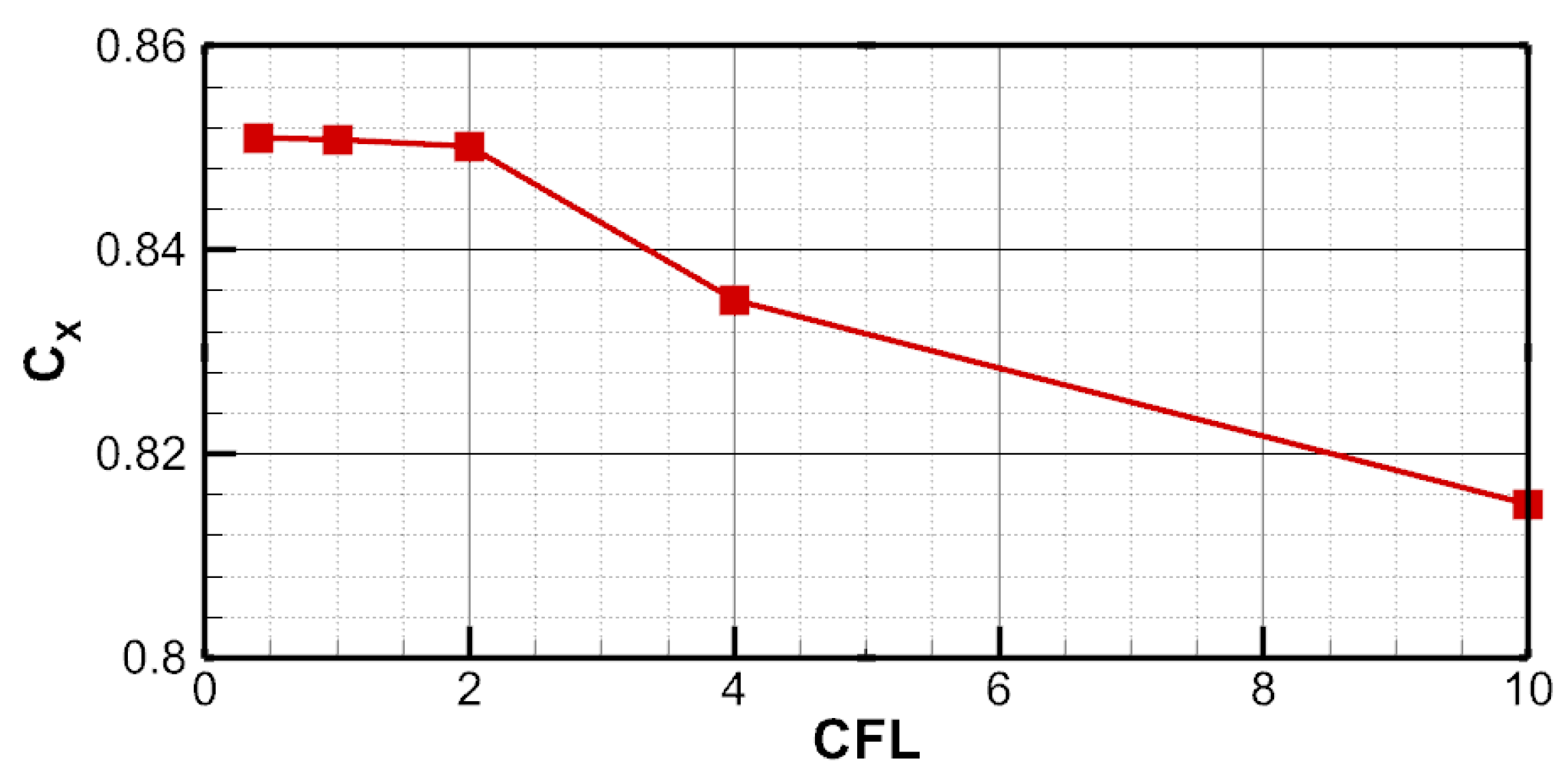
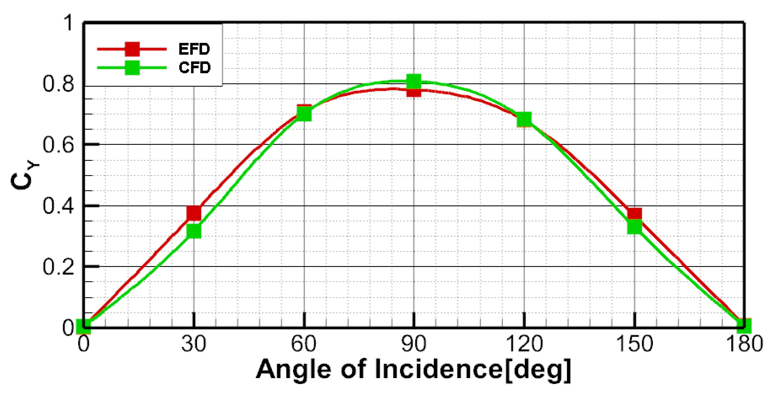
3.1. Grid Validation and Verification

| Case 1 | Case 2 | Case 3 | Case 4 | Case 5 | |
|---|---|---|---|---|---|
| CFL | 0.4 | 1 | 2 | 4 | 8 |
| Number of cells | 2.7 × 10⁷ | 2.1 × 10⁷ | 1.6 × 10⁷ | 1.1 × 10⁷ | 8 × 10⁶ |
3.2. Estimation of the Wind Force for Various Ships
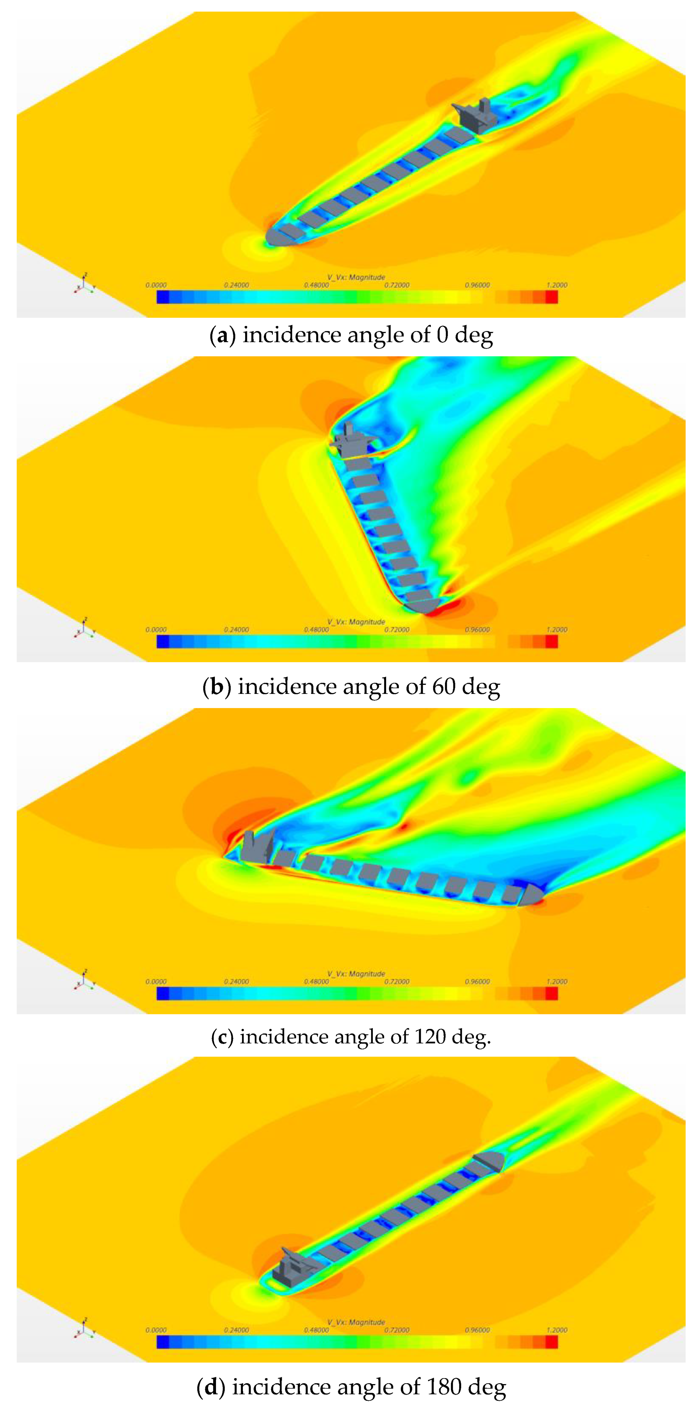
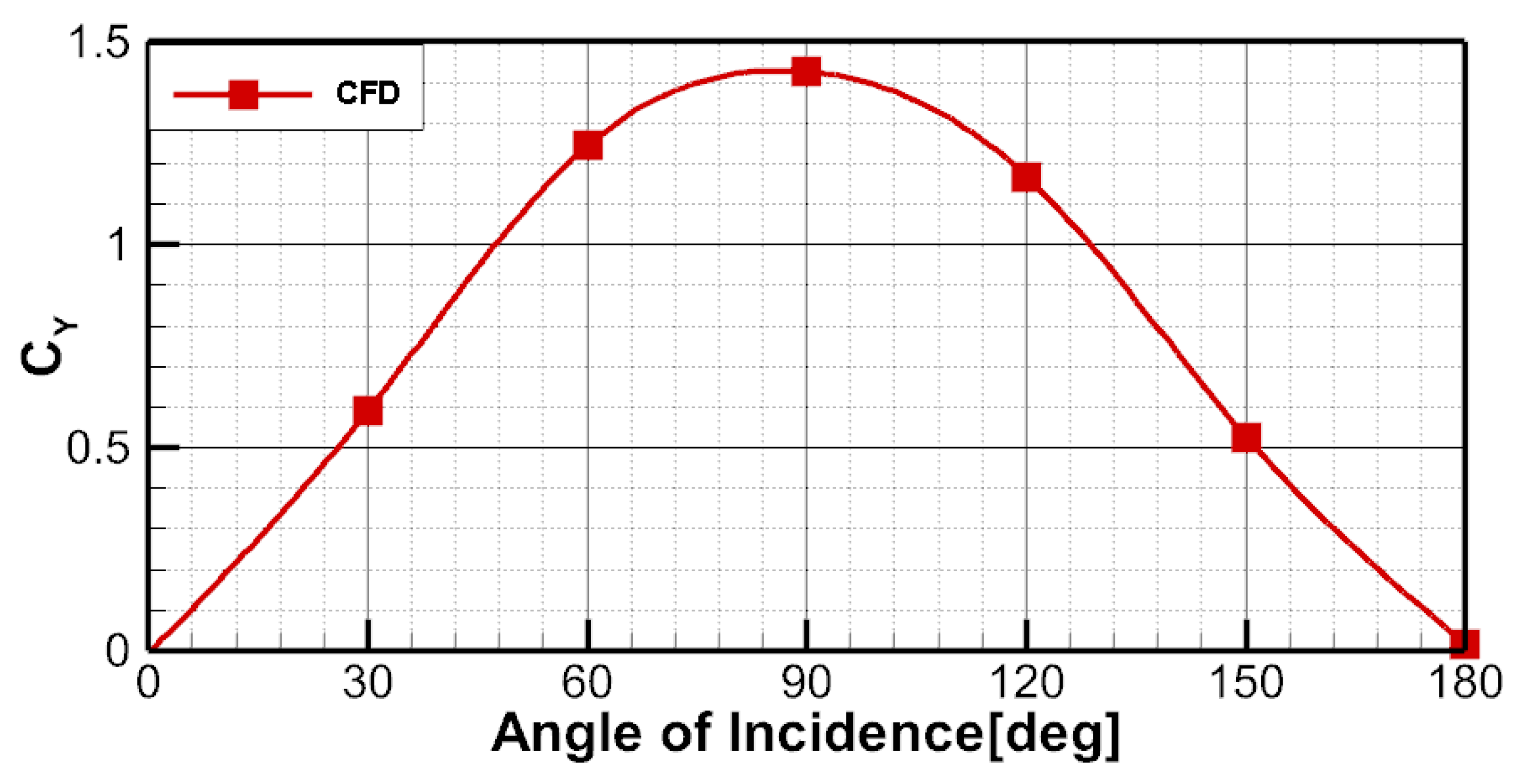
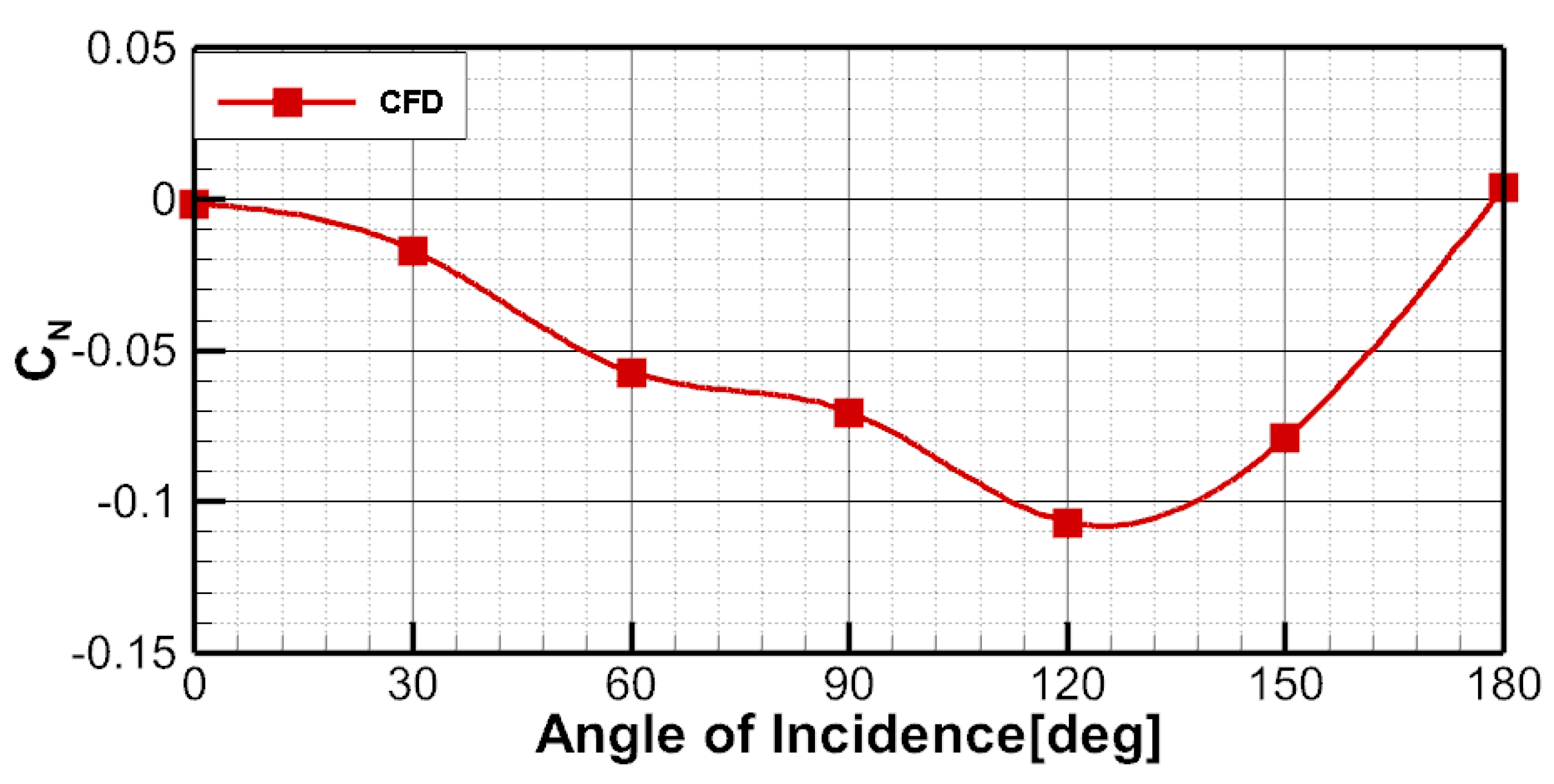
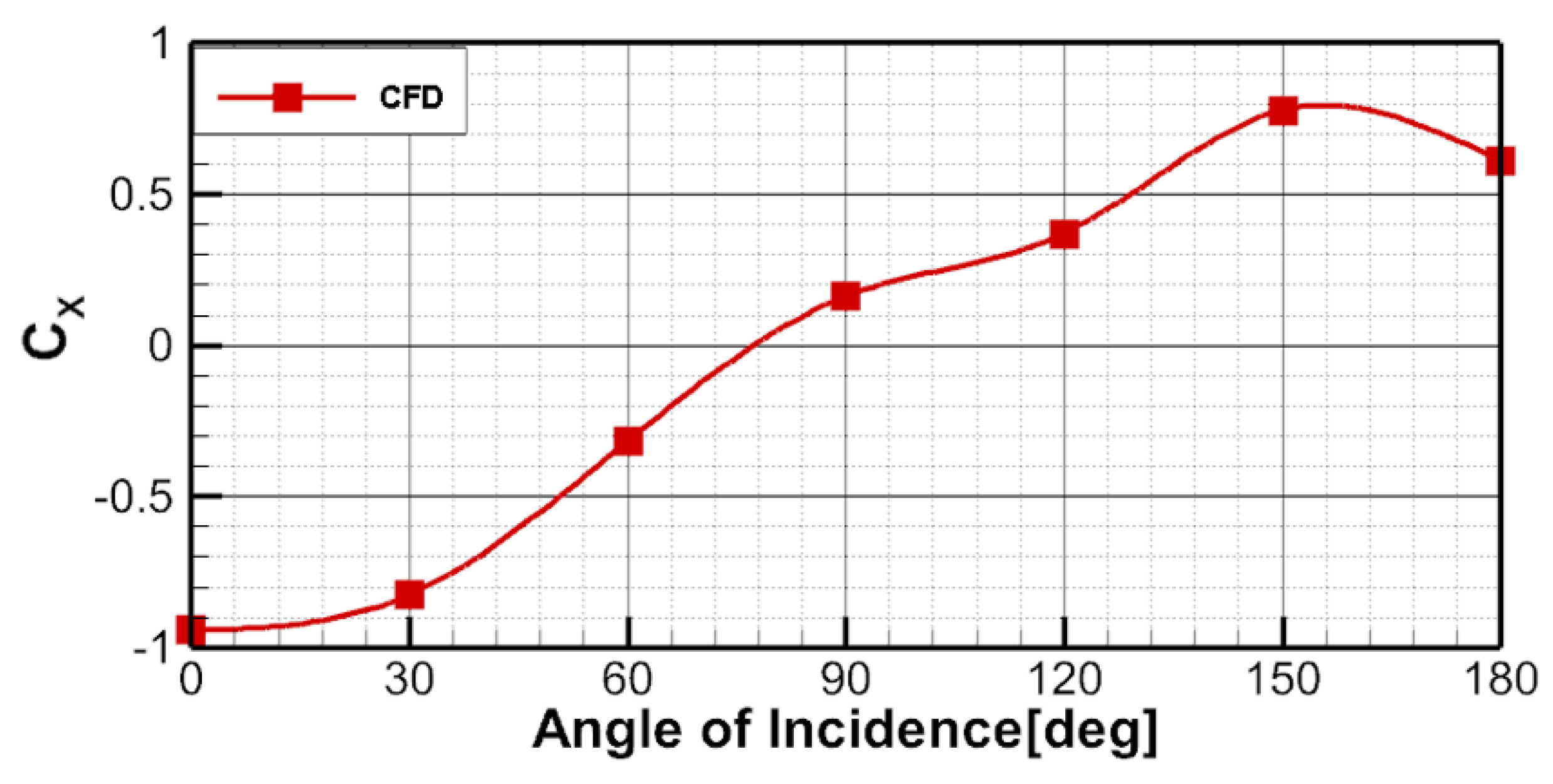
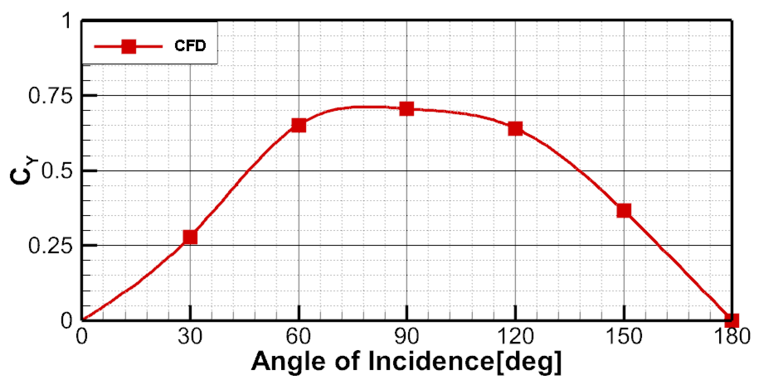
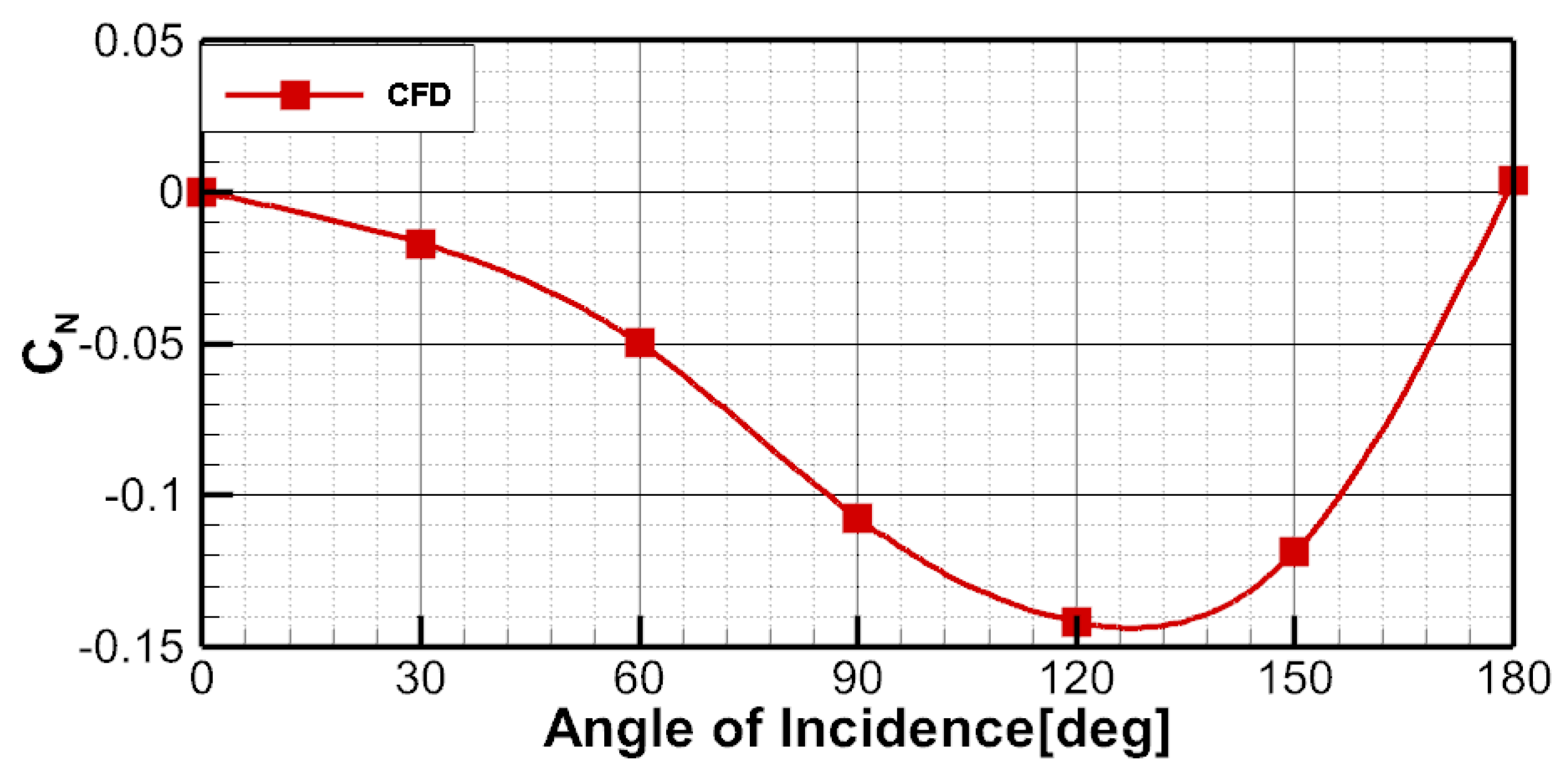
3.2.1. Wind Force of JBC Ship
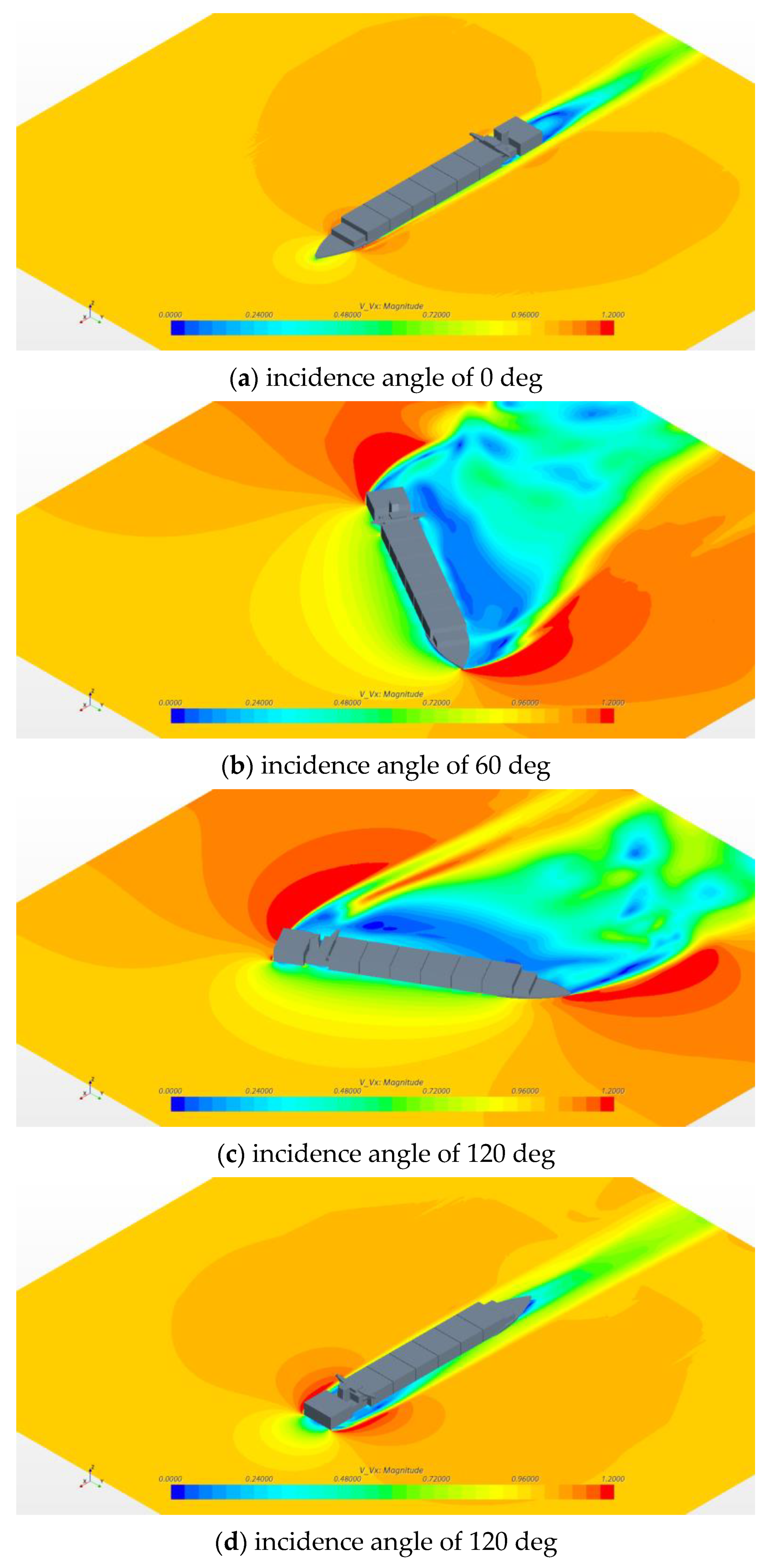
3.2.2. Wind Force of the KCS Ship
3.2.3. Wind Force of the KVLCC Ship
3.3. Estimation of Current Force for Various Ships
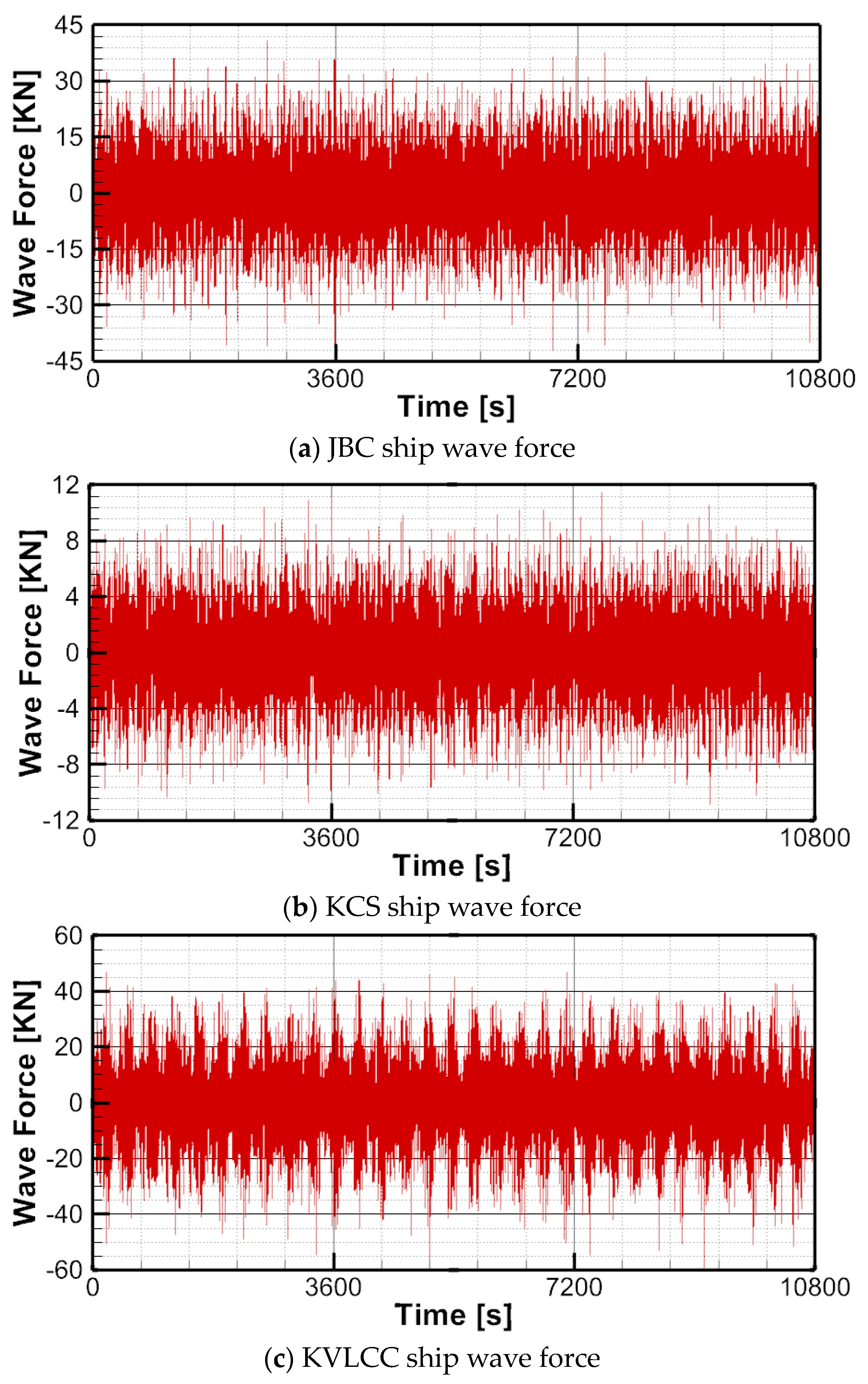
3.4. Estimation of Wave Force for Various Ships
3.5. Estimation of Total Mooring Force for Various Ships
4. Conclusions
Author Contributions
Funding
Institutional Review Board Statement
Informed Consent Statement
Data Availability Statement
Acknowledgments
Conflicts of Interest
References
- DNV; Li, Y. A New Look at Safe Mooring. 2020. Available online: https://www.dnv.com/expert-story/maritime-impact/A-new-look-at-safe-mooring.html (accessed on 18 June 2023).
- UK P&I Club. Risk Focus Consolidated 2016: Identifying Major Areas of Risk. 2016. Available online: https://kupdf.net/download/risk-focus-consolidated-2016_597efdfadc0d60ab762bb17e_pdf (accessed on 18 June 2023).
- Kuzu, A.C.; Arslan, Ö. Analytic comparison of different mooring systems. In Proceedings of the 18-th Annual General Assembly of the International Association of Maritime Universities—Global Perspectives in MET: Towards Sustainable, Green and Integrated Maritime Transport, Varna, Bulgaria, 11–14 October 2017; pp. 265–274. [Google Scholar]
- Popesco, O. Automating the Mooring Process. 2009. Available online: https://aapa.files.cmsplus.com/Seminar-Presentations/2009Seminars/09Facilities/09FACENG_Popesco_Ottonel1.pdf (accessed on 19 June 2023).
- Ma, K.; Shu, H.; Smedley, P.; L’hostis, D.; Duggal, A.S. A Historical Review on Integrity Issues of Perma Permanent Mooring Systems. In Proceedings of the Offshore Technology Conference, Houston, TX, USA, 6–9 May 2013; p. OTC-24025-MS. [Google Scholar]
- Van Bonifacio, J.; van der Meijden, F.; Sprenger, G.; Sproot, D. Alternative Berthing: Improvement and Innovation; Maritime Symposium: Roterdam, The Netherlands, 2014. [Google Scholar]
- Gao, F.; Hu, K.; Shen, W.J.; Li, Y. Study on the Safety Guarantee of Ship Mooring from Frequent Cable Accidents. In Proceedings of the IOP Conference Series: Earth and Environmental Science, Shenzhen, China, 23–25 October 2020; IOP Publishing Ltd.: Bristol, UK, 2021; Volume 621. [Google Scholar]
- Brindley, W. Mooring Rope Snapback Simulation. 2022. Available online: https://ore.catapult.org.uk/blog/mooring-rope-snapback-simulation/ (accessed on 19 June 2023).
- Shapovalov, K.A.; Shapovalova, P.K. Traumatism during Mooring Operations on Vessels. Ann. Mar. Sci. 2020, 4, 30–34. [Google Scholar] [CrossRef]
- The Maritime Executive. Majority of Mooring Accidents Caused by Lines Parting. 2015. Available online: https://maritime-executive.com/article/majority-of-mooring-accidents-caused-by-lines-parting (accessed on 19 June 2023).
- Erkan, Ç. Fatal and Serious Injuries on Board Merchant Cargo Ships. Int. Marit. Health 2019, 70, 113–118. [Google Scholar]
- Poisson, M. Safety Issues Associated with Mooring Operations in the Maritime Industry. 2017. Available online: https://www.tsb.gc.ca/eng/securite-safety/marine/2018/m17c0060/m17c0060.html (accessed on 19 June 2023).
- CHIRP Maritime. Maib Accident Reports Reference Library. 2022. Available online: https://chirp.co.uk/maritime/external-resources/ (accessed on 19 June 2023).
- Registry, C. Accidents and Incidents Reported to MACI (2020). 2021, pp. 1–12. Available online: https://www.cishipping.com/policy-advice/casualty-investigations (accessed on 19 June 2023).
- Yan, K.; Zhang, S.; Oh, J.; Seo, D.W. A Review of Progress and Applications of Automated Vacuum Mooring Systems. J. Mar. Sci. Eng. 2022, 10, 1085. [Google Scholar] [CrossRef]
- Cavotec. Automated Mooring. 2022. Available online: https://www.cavotec.com/en/your-applications/ports-maritime/automated-mooring (accessed on 19 June 2023).
- Cavotec. MoorMaster Automated Vacuum Mooring System. 2022. Available online: https://www.cavotec.com/en/video/moormaster-automated-vacuum-mooring-system (accessed on 19 June 2023).
- Mentjes, J.; Wiards, H.; Feuerstack, S. Berthing Assistant System Using Reference Points. J. Mar. Sci. Eng. 2022, 10, 385. [Google Scholar] [CrossRef]
- Chen, C.; Li, Y. Ship Berthing Information Extraction System Using Three-Dimensional Light Detection and Ranging Data. J. Mar. Sci. Eng. 2021, 9, 747. [Google Scholar] [CrossRef]
- Iris, Ç.; Lam, J.S.L. A Review of Energy Efficiency in Ports: Operational Strategies, Technologies and Energy Management Systems. Renew. Sustain. Energy Rev. 2019, 112, 170–182. [Google Scholar] [CrossRef]
- Iris, Ç.; Lam, J.S.L. Optimal Energy Management and Operations Planning in Seaports with Smart Grid While Harnessing Renewable Energy under Uncertainty. Omega 2021, 103, 102445. [Google Scholar] [CrossRef]
- Iris, Ç.; Lam, J.S.L. Recoverable Robustness in Weekly Berth and Quay Crane Planning. Transp. Res. Part B Methodol. 2019, 122, 365–389. [Google Scholar] [CrossRef]
- Andersen, I.M.V. Wind Loads on Post-Panamax Container Ship. Ocean Eng. 2013, 58, 115–134. [Google Scholar] [CrossRef]
- Wang, W.; Wu, T.; Zhao, D.; Guo, C.; Luo, W.; Pang, Y. Experimental–Numerical Analysis of Added Resistance to Container Ships under Presence of Wind–Wave Loads. PLoS ONE 2019, 14, e0221453. [Google Scholar] [CrossRef] [PubMed]
- Ricci, A.; Janssen, W.D.; van Wijhe, H.J.; Blocken, B. CFD Simulation of Wind Forces on Ships in Ports: Case Study for the Rotterdam Cruise Terminal. J. Wind Eng. Ind. Aerodyn. 2020, 205, 104315. [Google Scholar] [CrossRef]
- Zhou, Y.; Daamen, W.; Vellinga, T.; Hoogendoorn, S.P. Impacts of Wind and Current on Ship Behavior in Ports and Waterways: A Quantitative Analysis Based on AIS Data. Ocean Eng. 2020, 213, 107774. [Google Scholar] [CrossRef]
- Kobayashi, H.; Kume, K.; Orihara, H.; Ikebuchi, T.; Aoki, I.; Yoshida, R.; Yoshida, H.; Ryu, T.; Arai, Y.; Katagiri, K.; et al. CFD Assessment of the Wind Forces and Moments of Superstructures through RANS. Appl. Ocean Res. 2022, 129, 103364. [Google Scholar] [CrossRef]
- Martić, I.; Degiuli, N.; Farkas, A.; Gospić, I. Evaluation of the Effect of Container Ship Characteristics on Added Resistance in Waves. J. Mar. Sci. Eng. 2020, 8, 696. [Google Scholar] [CrossRef]
- Sasa, K.; Incecik, A. Numerical Simulation of Anchored Ship Motions due to Wave and Wind Forces for Enhanced Safety in Offshore Harbor Refuge. Ocean Eng. 2012, 44, 68–78. [Google Scholar] [CrossRef]
- Lee, K.H.; Han, H.S.; Park, S. Failure Analysis of Naval Vessel’s Mooring System and Suggestion of Reducing Mooring Line Tension under Ocean Wave Excitation. Eng. Fail. Anal. 2015, 57, 296–309. [Google Scholar] [CrossRef]
- Lin, J.F.; Zhao, D.G.; Guo, C.Y.; Su, Y.M.; Zhong, X.H. Comprehensive test system for ship-model resistance and propulsion performance in actual seas. Ocean Eng. 2020, 197, 106915. [Google Scholar] [CrossRef]
- Farkas, A.; Degiuli, N.; Martić, I. Assessment of Hydrodynamic Characteristics of a Full-Scale Ship at Different Draughts. Ocean Eng. 2018, 156, 135–152. [Google Scholar] [CrossRef]
- Larsson, L.; Stern, F.; Visonneau, M.; Hino, T.; Hirata, N.; Kim, J. Tokyo 2015 Workshop on CFD in Ship Hydrodynamics; National Maritime Research Institute: Tokyo, Japan, 2015. [Google Scholar]
- Gang, J.G.; Lee, J.W. Report on Research and Development Services for Marine Repair Phenomena in Busan New Port (5th Phase); Ministry of Land, Transport and Maritime Affairs: Busan, Republic of Korea, 2011; pp. 45–55. [Google Scholar]
- Grlj, C.G.; Degiuli, N.; Tuković, Ž.; Farkas, A.; Martić, I. The Effect of Loading Conditions and Ship Speed on the Wind and Air Resistance of a Containership. Ocean Eng. 2023, 273, 113991. [Google Scholar] [CrossRef]
- ISO 15016(2016); Ships and Marine Technology—Guidelines for the Assessment of Speed and Power Performance by Analysis of Speed Trial Data. ISO: Geneva, Switzerland, 2015.
- ANSYS Inc. Aqwa Theory Manual; ANSYS Inc.: Canonsburg, PA, USA, 2021; pp. 21–55. Available online: https://www.ansys.com (accessed on 17 August 2023).
- Ministry of Ocean and Fisheris. Port and Fishing Port Design Criteria, 2014, 111-1192000-000184-14, Republic of Korea. Available online: https://www.mof.go.kr/en/index.do (accessed on 17 August 2023).
- ANSYS Inc. Aqwa User’s Manual Third-Party Software; ANSYS Inc.: Canonsburg, PA, USA, 2021; Available online: https://www.ansys.com (accessed on 17 August 2023).
- Kume, K.; Hamada, T.; Kobayashi, H.; Yamanaka, S. Evaluation of Aerodynamic Characteristics of a Ship with Flettner Rotors by Wind Tunnel Tests and RANS-Based CFD. Ocean Eng. 2022, 254, 111345. [Google Scholar] [CrossRef]


| Main Particulars | JBC | KCS | KVLCC | |
|---|---|---|---|---|
| Length Overall (LOA) | m | 291.3 | 232.5 | 325.5 |
| Length Between Perpendicular (LBP) | m | 280 | 230 | 320 |
| Breadth (B) | m | 45 | 32.2 | 58 |
| Mean Draft (Fully loaded condition) | m | 25 | 19 | 30 |
| Transverse Projected Area | m2 | 964 | 839 | 1085 |
| Lateral Projected Area | m2 | 3364 | 4975 | 2665 |
| Displacement (Fully loaded condition) | m3 | 178,370 | 52,030 | 312,738 |
| Block Coefficient (Cb) | 0.86 | 0.65 | 0.81 | |
| GM (Fully loaded condition) | m | 5.32 | 0.62 | 0.65 |
| JBC | KCS | KVLCC | |||||
|---|---|---|---|---|---|---|---|
| Vwind m/s | RX [KN] | RY [KN] | RX [KN] | RY [KN] | RX [KN] | RY [KN] | |
| Wind force | 14 | 0.5 | 340 | 23 | 838 | 20 | 222 |
| 30 | 2.3 | 1674 | 117 | 4118 | 102 | 1091 | |
| JBC | KCS | KVLCC | |||||
|---|---|---|---|---|---|---|---|
| Vcurrent m/s | RX [KN] | RY [KN] | RX [KN] | RY [KN] | RX [KN] | RY [KN] | |
| Current force | 1 | 8.2 | - | 3.9 | - | 11.4 | - |
| JBC | KCS | KVLCC | ||||
|---|---|---|---|---|---|---|
| FX [kN] | FY [kN] | FX [kN] | FY [kN] | FX [kN] | FY [kN] | |
| Wind force | 0.5 | 340 | 23 | 838 | 20 | 222 |
| Current force | 8.2 | - | 3.9 | - | 11.4 | - |
| Wave force | 32.5 | 11.8 | 45.8 | |||
| Total force | 41.2 | 340 | 38.7 | 837 | 77.2 | 222 |
| JBC | KCS | KVLCC | ||||
|---|---|---|---|---|---|---|
| FX [kN] | FY [kN] | FX [kN] | FY [kN] | FX [kN] | FY [kN] | |
| Wind force | 2.3 | 1674 | 117 | 4188 | 102 | 1091 |
| Current force | 8.2 | - | 3.9 | - | 11.4 | - |
| Wave force | 32.5 | 11.8 | 45.8 | |||
| Total force | 43 | 1674 | 132.7 | 4188 | 159.2 | 1091 |
Disclaimer/Publisher’s Note: The statements, opinions and data contained in all publications are solely those of the individual author(s) and contributor(s) and not of MDPI and/or the editor(s). MDPI and/or the editor(s) disclaim responsibility for any injury to people or property resulting from any ideas, methods, instructions or products referred to in the content. |
© 2023 by the authors. Licensee MDPI, Basel, Switzerland. This article is an open access article distributed under the terms and conditions of the Creative Commons Attribution (CC BY) license (https://creativecommons.org/licenses/by/4.0/).
Share and Cite
Yan, K.; Oh, J.; Seo, D.-W. Computational Analysis for Estimation of Mooring Force Acting on Various Ships in Busan New Port. J. Mar. Sci. Eng. 2023, 11, 1649. https://doi.org/10.3390/jmse11091649
Yan K, Oh J, Seo D-W. Computational Analysis for Estimation of Mooring Force Acting on Various Ships in Busan New Port. Journal of Marine Science and Engineering. 2023; 11(9):1649. https://doi.org/10.3390/jmse11091649
Chicago/Turabian StyleYan, Kaicheng, Jungkeun Oh, and Dae-Won Seo. 2023. "Computational Analysis for Estimation of Mooring Force Acting on Various Ships in Busan New Port" Journal of Marine Science and Engineering 11, no. 9: 1649. https://doi.org/10.3390/jmse11091649