Route Planning of a Polar Cruise Ship Based on the Experimental Prediction of Propulsion Performance in Ice

Abstract

The effective assessment of risk and speed limitations in ice are critical for the route planning of polar cruise ships. While the Polar Operational Limit Assessment Risk Indexing System (POLARIS) is widely used to evaluate the operational risk in ice, its scope of assessment is limited to the ship’s assigned ice class. For a specific ship with a given ice class, the propulsion performance under varying ice conditions is more essential for assessing the besetting risk and finding an optimal route. To establish a more detailed risk evaluation method for a PC6 class polar cruise ship, propulsion performance under various ice conditions is obtained via model tests in an ice tank. During the tests, the tow force, propeller torque, and thrust are measured under different ship velocities and propeller rotation rates, and the relations between required delivered power (P) and ship velocity (V) under the tested ice thicknesses and concentrations are obtained and extended to other ice conditions by curve fitting. A new risk index outcome, RIO*, is proposed after POLARIS according to the optimized load ranges of the ship’s rated power. Four risk levels, including low, medium, high, and unnavigable, are classified with the required propulsion power in ice being 50%, 85%, 100%, and >100% of the rated power, respectively. The recommended speed limit for each risk level is proposed based on the economical service speed of 11 kn, the operational limit of 3 kn by POLARIS and the minimum speed of 0.5 kn to avoid besetting, respectively. Based on the RIO* and P–V relations, the speed map for varying ice thicknesses and concentrations can be calculated. On these bases, a route planning simulation for the present polar cruise ship is performed. Results of the case study show that 29% of the simulated area is identified as “unnavigable” by the present procedure, while only 8% is detected by POLARIS.

1. Introduction

The unique scenery and adventure in polar regions have attracted humans for many years. Antarctic tourism began in the 1950s. With the improvements in technologies of transportation and communication, Antarctic tourism has continued to develop—the number of visitors in Antarctica increased by 27% annually from 1992 to 2019 [1]. During the years 2018–2019, a total of 55,489 people arrived in Antarctica, among which the tourists from the United States accounted for the largest percentage (32%), and tourists accounted for the second (15%) [2]. Antarctica has unique landscapes and animal life, including ice shelves, icebergs, ice sheets, auroras, penguins, walruses, seals, and whales. The Antarctic Peninsula has the richest landscape resources and is also the region with the highest number of Antarctic tourists [3]. Additionally, the number of tourists to the Arctic is growing rapidly [4]. The tourism industry has brought billions of dollars in economic benefits to the Arctic region, and its development has become a major goal for the indigenous economies of Greenland, Greenland, Nunavut, the Yukon region, the Russian Federation, and Alaska [5,6]. The launches and deliveries of series of PC6 classed polar expedition cruise ships, from Greg Mortimer in 2019 to the fifth sister ship Ocean Odyssey in 2022, and also saw a boom in the polar tourism market.

Polar expeditions face the problem of ships navigating through ice-covered waters. To ensure safety in the ice and assist the decision making of the ship’s master or watchkeeping crew, prior route planning is required. For open-water merchant ships, economic efficiency is the main purpose, i.e., the route planning should minimize the voyage time and reduce the fuel consumption. However, for polar cruise ships, the aim is to provide the experience of navigating and sightseeing in ice-covered areas to the tourists as much as possible with safety ensured. Considering that sea ice is the main obstacle that increases the ship resistance and sometimes causes besetting incidents [7], an accurate assessment of the ship’s performance in ice and a detailed route planning method based on the clear understanding and reliable evaluation of ice risks are fundamental guarantees for the safety and efficiency of polar cruise ships.

At present, the Polar Operational Limit Assessment Risk Indexing System (POLARIS) established by the International Maritime Organization (IMO) is most widely used among the methodologies for assessing navigation risks and speed limitations in ice [8,9,10,11]. POLARIS was developed by integrating multiple methodologies including the Arctic Ice Regime Shipping System of Canada, the Russian Ice Certificate, and the Rules of Navigation on the water area of the Northern Sea Route [12]. POLARIS utilizes the Risk Index Outcome (RIO) values to limit ship’s operations in ice. The value of RIO is determined by a summation of the Risk Index Values (RIVs), which are assigned to the ship based on ice class and ice type, with each ice type present in the ice regime multiplied by its concentration (expressed in tenths). POLARIS classifies three levels of operation, including normal operation (RIO ≥ 0 with no speed limitation), elevated operational risk (−10 < RIO ≤ 0 with speed limitation related to ice class), and operation subject to special consideration (RIO < −10 with icebreaker escort required or voyage avoided). However, for the route planning with ice data of limited resolution, one problem is that there may be only one ice type in a localized area (e.g., Medium First Year Ice less than 1 m thick), and the POLARIS degenerates to the point that the operational risk is evaluated by ice thickness only, while weakening the influence of sea ice concentration, which is obviously not sufficient for route planning for polar cruise ships with finite propulsion power. Such consideration also stems from the apprehension of some captains regarding the results of risk estimates from POLARIS, which permit navigation in hazardous ice areas beyond the ship’s capability [13]. Therefore, it is necessary to establish a continuous mapping relationship between various ice conditions and safe speeds based on the propulsion performance of the ship in ice, rather than recommending a single speed limitation for a wide range of ice conditions as POLARIS.

The study of route planning generally includes optimization models, performance evaluation models (speed design and optimization), path finding models, data structures, etc. (e.g., [14]). For a specific ship especially facing complex ice conditions, speed design and optimization based on sea ice data has become a critical part of route planning [11,15,16,17]. Often, semi-empirical formula or historical operational data could be the reference for determining the ship’s speed navigating through ice. However, polar cruise ships with lower ice classes (e.g., PC6) are generally not equipped with ice-breaking bow forms, and the traditional semi-empirical formula may be no longer applicable. Additionally, open access ice navigation data of similar ships are very limited. Given the above situation, scaled model tests in an ice tank can be a preferred alternative solution for the prediction of a ship’s propulsion performance in ice, which is also the recommended practice in ice class rules or relevant international standards (e.g., [18,19]).

In the present study, the propulsion performance and besetting risk of a PC6 classed polar cruise ship under different ice conditions are examined via model tests in an ice tank. Detailed risk index and speed design methods for ice navigation are proposed based on the test results. Additionally, route planning simulation and analysis for potential itineraries in the Antarctic regions are conducted as a case study.

2. Propulsion Tests in Ice Tank

As mentioned above, POLARIS can be a basic guidance for assessing the operational risks in polar waters, but it has not yet been matched to the propulsive capabilities of a specific ship. For the PC6 classed polar cruise ship discussed in this paper, the RIV of “Medium First Year Ice less than 1 m thick” is +1, and the calculated RIO would always be greater than 0 regardless of ice concentration if there are no heavier ice types in the ice regime, which suggests “normal operation”. However, even in the so-called “normal operation” level, the polar cruise ship may become stuck in concentrated pack ice. To avoid possible besetting incidents under specific propulsion power, the speed design of the ship should be evaluated for more detailed sea ice conditions including thickness and concentration. On the other hand, level ice breaking is beyond the operation scenarios of the present PC6 classed ship and will not be discussed in this paper. Thus, the model tests presented hereinafter are carried out under pack ice conditions of different thicknesses and concentrations.

2.1. Test Facility and Ship Model

The present tests are performed in the ice tank at the Ice Mechanics and Engineering Laboratory of Tianjin University, which is 40 m (long) × 6 m (wide) × 2.0 m (deep) with a cooling system sending cold air from the top of the insulated room that can be cooled down to an air temperature of −22 °C. By varying the room’s air temperature, ice sheets can be grown, tempered or melted. The main carriage on the tank is designed for loads up to 5 tons. It can move a given distance at a constant speed, ranging from 1 mm/s to 1000 mm/s. The service carriage on the tank is used to assist the production and property measurements of the model ice.

As mentioned above, the full-scale ship discussed in the present study is a polar expedition cruise ship with a PC6 class notation. The ship can carry up to 200 guests and offer a smooth ride in harsh waters using the X-BOW design. The model ship is built to be a correct geometric representation of the full-scale ship at the scale ratio of 1:20, as shown in Figure 1. The primary dimensions of the present ship in both scales are listed in

Table 1. Primary dimensions of the polar cruise ship in full and model scale.

Parameters	Full Scale	Model Scale
Length overall	104.4 m	5.22 m
Breadth	18.4 m	0.92 m
Drought for upper ice waterline (UIWL)	5.55 m	0.2775 m
Displacement at UIWL	6646 ton	0.831 ton
Rated power	4.0 MW	/

. The model ship is towed by a steel rod attached to the main carriage by a universal joint, and the connection between the rod and the ship is based on a spherical plain bearing and a load cell. This load cell is used to measure the towing force of the ship. The signals from this sensor are recorded by the data acquisition system and sampled at a rate of 100 Hz. Two transverse springs are mounted on the rod near the bow of the model ship to avoid possible excessive course deviations, and turnbuckles are used to adjust the tautness of the springs. Under such configuration, the model ship is practically free to heave, pitch and roll and also allowed to sway and yaw within a limited range. The full-scale ship is propelled by two four-bladed propellers with a diameter of 3.1 m and rated rotation speed of 201.5 r/min. According to the recommended procedure of the International Towing Tank Conference (ITTC) for propulsions tests in ice, the required propeller shaft power in ice is derived based on the thrust and torque measurements at the self-propulsion point [20]. Thus, two dynamometers are mounted in the ship model to measure the shaft thrust and torque. A sample rate of 100 Hz is set for the dynamometers during the tests. The main specifications of the measuring devices are listed in

Table 2. Main specifications of the measuring devices used in the model tests.

Test Parameters	Measuring Device	Range	Accuracy
Towing force	One-directional load cell	0–3000 N	±1.5 N
Shaft thrust	Dynamometer	0–2000 N	±1.0 N
Shaft torque	Dynamometer	0–10 Nm	±0.01 Nm
Propeller rate	Servo motor	0–3000 r/min	0.1 r/min
Ship velocity	Main carriage	0–1.0 m/s	1 mm/s

.

2.2. Model Ice

Urea model ice is used in the present tests. Detailed generating process and strength measurements of model ice can be found in [21,22]. Model ice is dominated by a columnar crystal structure, as shown in Figure 2, which is also the main characteristic of the first-year sea ice in the Arctic and part of Antarctica [23,24].

2.3. Scaling Laws

Froude and Cauchy scaling laws have been widely accepted in the physical modeling of ships breaking ice (see, e.g., [19,25,26]). During the navigation in pack ice, the ship impacts the ice floes at a certain mass and speed, where the gravity and inertia forces govern the process. Meanwhile, ice floes may fail in local crushing, bending or splitting, where the elastic forces predominate. The Froude number Fr and Cauchy number Ca are calculated by:

$$Fr=\frac{V}{\sqrt{gL}}$$

(1)

$$Ca=\frac{\rho V^2}{E}$$

(2)

where V is the velocity, g the acceleration of gravity, L the geometric length, ρ the density, and E the elastic modulus of ice.

Based on the maintenance of both Froude and Cauchy numbers in both full and model scales, the ice thickness, strength, and elastic modulus are scaled by λ (i.e., the geometric scale factor; set as 20 in the present tests), the time and velocity by λ^1/2, the mass and force by λ³, and the torque by λ⁴.

2.4. Test Conditions and Procedure

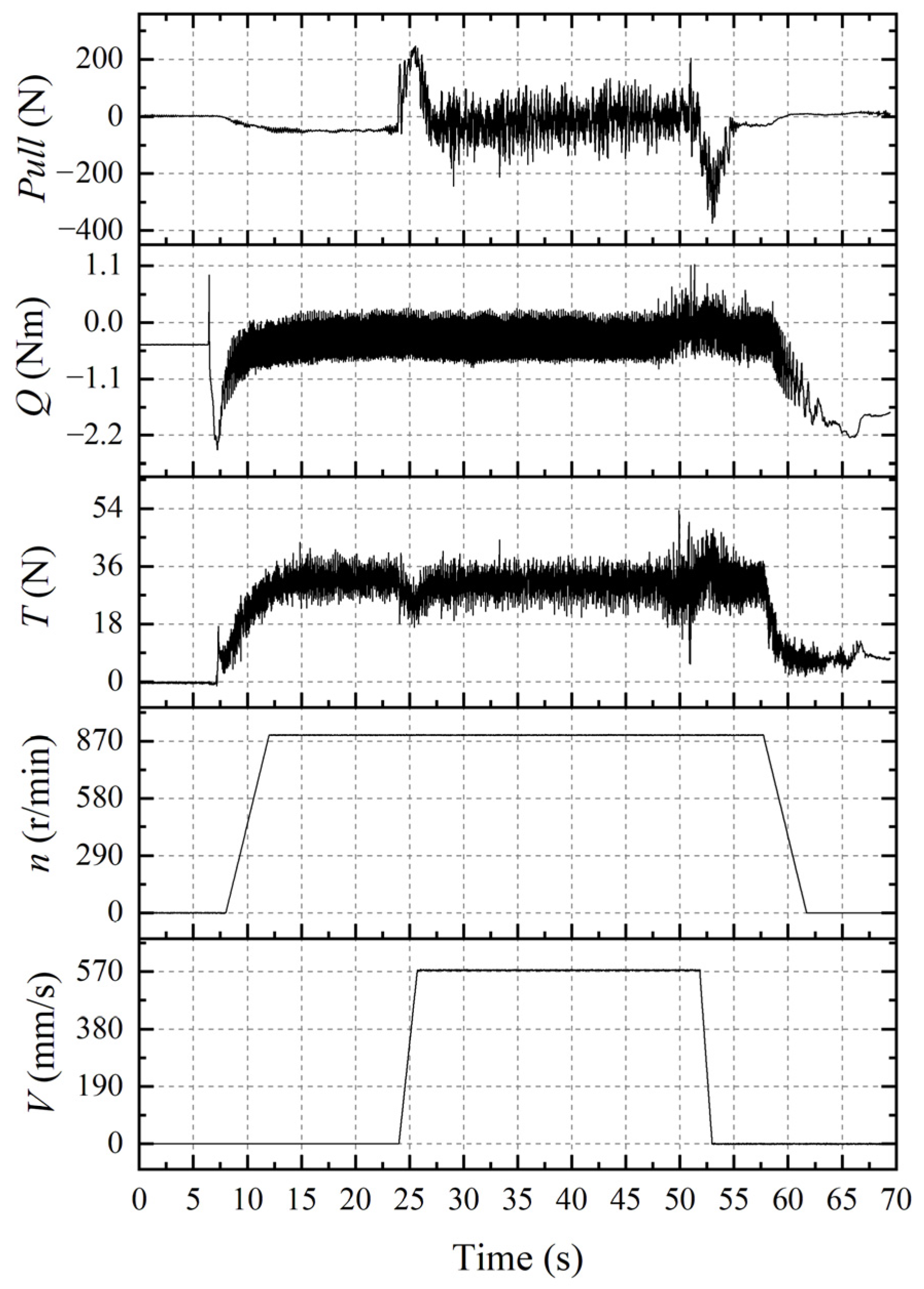
To predict the required power for ice navigation, the first step is to find the self-propulsion point, where the towing force reaches to zero and the thrust balances with the resistance in ice. However, a direct acquisition of the self-propulsion point is challenging due to the significant fluctuations in ice resistance resulting from the deviations of floe size, shape, local concentration, as well as the nonsimultaneous ice contact and failure. Recommended practice is to set several propeller rotation rates below and above the self-propulsion point, respectively, and use curve fitting and interpolation to find the point corresponding to zero towing force [20]. To assist the decision making on the selection of suitable propeller rates, resistance tests in ice and bollard pull tests are carried out in advance. The test conditions are listed in

Table 3. Test conditions for the present ship.

Scale	Ice Thickness	Ice Concentration	Ship Velocity
Full-scale	1.0 m, 0.5 m	90%, 70%, 50%	3 kn, 5 kn, 8 kn
Model-scale	5.0 cm, 2.5 cm	90%, 70%, 50%	0.345 m/s, 0.575 m/s, 0.920 m/s

, with full-scale and model-scale target values included. Three full-scale ship velocities are selected for the present tests, including 3 kn (i.e., the recommended speed limit for ice class below PC5 under elevated-risk operation by POLARIS), 8 kn (i.e., a velocity that may be sufficiently high to exceed the ship’s propulsion capability in ice), and 5 kn in between. The flexural strength of ice in full scale is selected as 500 kPa, and the target value for the parental model ice sheet is 25 kPa. For each combination of ice thickness, concentration and ship velocity, a total of four propeller rates are tested, including 0 r/min for the resistance test.

During each test, the model ship is firstly loaded to the upper ice waterline. Meanwhile, the parental model ice sheet is immediately cut into floes with required sizes and concentration after the desired flexural strength is reached. The maximum floe size is kept as two times the model ship breadth to minimize the side wall effect [27] and retain appropriate number of ice failure events. Then, the model ship is towed through the pack ice area at the desired velocity and propeller rate. To achieve the sufficiency and relatively steady state of the test data, the towing distance in each test run is set as four times the model ship length. For each test run a video camera is used to record the rotation or failure of ice floes.

2.5. Test Results

Figure 3 shows the ship–ice interaction scenario for ice concentrations of 50% and 90%, respectively. Higher ice concentrations are found to result in more floe splitting or cracking events, thereby increasing the ice resistance and requiring more delivered power. An example of the recorded time series of the towing force, propeller rate, velocity, shaft thrust, and torque of the model ship is presented in Figure 4. The time interval for the calculation of the average values of towing force, thrust and torque is chosen after one model length into the pack ice [28]. The determination of the self-propulsion point has been mentioned above, and the required shaft power for each test combination is calculated by [20]:

$$P_D=2\pi nQ$$

(3)

where P_D is the required shaft power, n the propeller rate of the self-propulsion point, and Q the shaft torque of the self-propulsion point. The results are then scaled up to full scale by Froude and Cauchy similarity. The predicted required propulsion powers for different conditions are listed in

Table 4. Predictions of required propulsion power in full scale based on model tests. The propulsion power is obtained under the self-propulsion point for each ship/ice condition, respectively.

Ice Concentration	Ship Velocity V (kn)	Required Propulsion Power PD (MW)
		Ice Thickness H = 0.5 m	Ice Thickness H = 1.0 m
90%	3	2.052	4.995
	5	2.673	5.679
	8	3.929	7.295
70%	3	1.280	2.909
	5	1.704	3.471
	8	2.805	4.909
50%	3	0.513	0.627
	5	0.722	0.919
	8	1.496	1.717

.

The results show that the required propulsion power increases with ship velocity, ice thickness, and concentration. As can be seen from Table 4, the required propulsion power under pack ice thickness 1.0 m, ice concentration 90% and ship velocity 8 kn has reached 7.295 MW, approximately 1.8 times the ship’s rated power (4.0 MW). Additionally, the required power at 3 kn under the same ice thickness and concentration exceeds the rated power, which indicates highly possible besetting accidents under such heavy ice condition. However, POLARIS suggests “normal operation” and recommends no speed limit for the present PC6-classed ship under the above-ice condition, which implies that the route planning in ice-covered waters based on POLARIS only may not be sufficient to ensure the operational safety of the ship, particularly when facing relatively severe ice conditions. Therefore, it is essential to define more specific risk levels linking to the propulsion performance of the ship in ice.

3. Risk Assessment and Speed Design Based on Propulsion Performance

3.1. P–V Relations Based on Test Results

For the route planning and operational risk assessment in continuously changing ice conditions, the prediction of propulsion performance for individual ice thickness and concentration is not sufficient as input. To evaluate the propulsion performance of the present ship in detail, the P–V relation is introduced, where P is short for power and V velocity. In this study, the P–V relation for each ice condition is preliminarily expressed by the exponential function:

$$P_D=A\cdot \exp \left(B\cdot V\right)$$

(4)

where P_D is the required shaft power of the propellers; A and B are related to ice thickness H and ice concentration C, and V is the ship velocity. For this function, the ice thickness H and concentration C are continuous variables, but only several ice conditions are tested due to the limitations of time and cost.

To ensure the reliability of the P–V relation model, a reasonable bound should be adopted before the extrapolation to other ice conditions based tested results. Figure 5 presents the variations in the predicted power with ship velocity under different ice thickness and concentration based on the tested data from Table 4. The least squares method is used to provide the best fit according to the exponential function of Equation (4). The results indicate that a decrease in ice thickness and concentration at the same ship velocity leads to a corresponding decrease in required shaft power. Therefore, open water conditions are used as the lower bound for the P–V model. For the present ship, the full and economic service speeds in open water are 16.5 kn and 11.0 kn, respectively, corresponding to 100% and 25% of the rated power. After applying the exponential function fitting to the open water P–V relation, the P–V curve groups used for the extrapolation are presented in Figure 6.

On these bases, the fitted surfaces of A and B in Equation (4) as functions of H and C are obtained (as plotted in Figure 7) and expressed in Equation (5).

$$\{\begin{array}{c}A=0.1435\exp \left(3.472H\cdot C\right)+13.94\exp \left[{\left(0.4314C\right)}^3\right]-14.06\\ B=-0.0161\exp \left(0.6386\pi \cdot H\cdot C\right)+0.1131\exp \left[{\left(-1.51C\right)}^3\right]+0.1583\end{array}$$

(5)

where definitions for A, B, H, and C remain the same as the above.

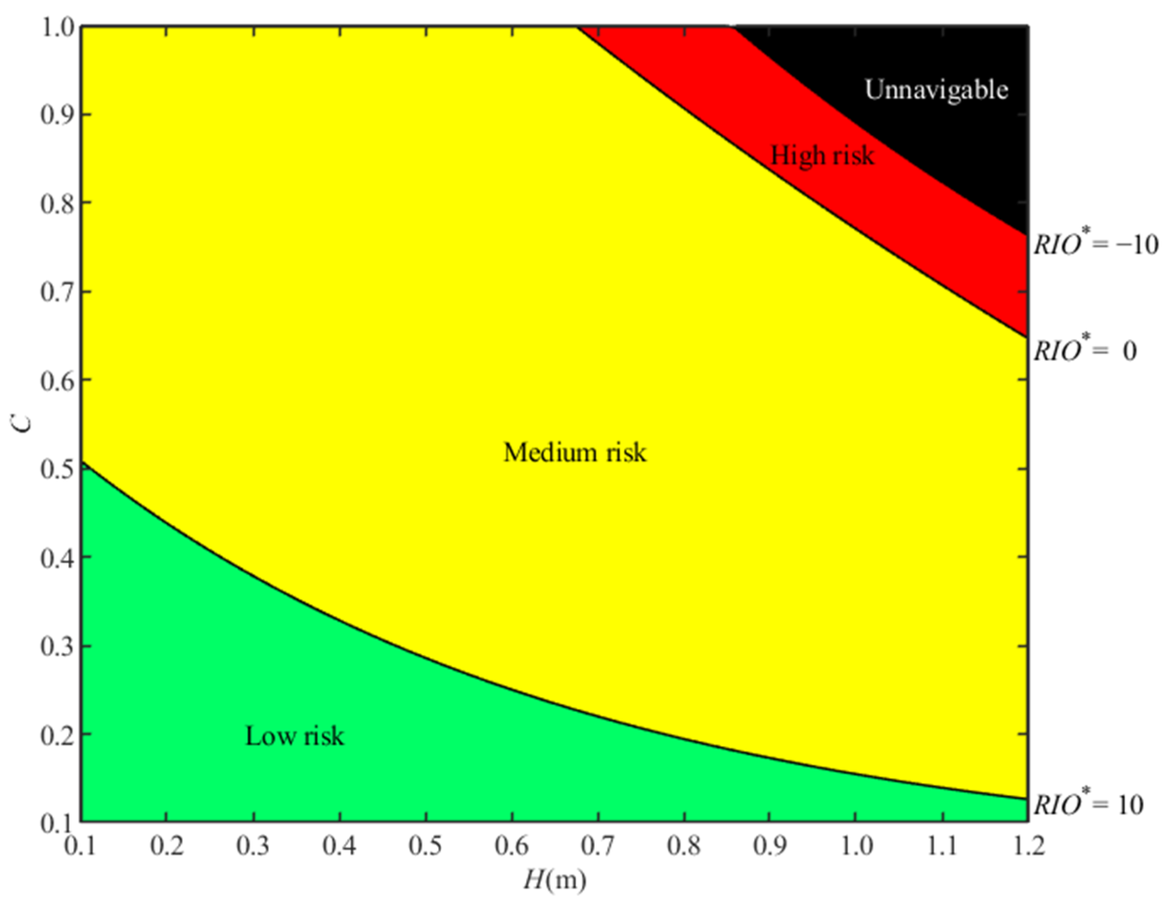
3.2. P_D-Based Navigational Risk Levels

The above test results show that increasing ice thickness and concentration result in higher required shaft power and potential higher besetting risk. However, the ship’s propulsion capacity has an upper limit, which is the rated power of 4 MW. Therefore, linking the risk levels to the required propulsion power is a straightforward way to evaluate the navigational risk in ice. According to MAN Diesel & Turbo, the thresholds for part and high engine load correspond to 50% and 85% of the Specified Maximum Continuous Rating (SMCR) [29]. These percentages are also used to define the risk levels in this study, as listed in

Table 5. Specific risk levels based on required propulsion power in ice.

Risk Level	Engine Load Range	PD in MW	RIO*
Low risk	≤50% SMCR	PD ≤ 2.0	RIO* ≥ 10
Medium risk	50–85% SMCR	2.0 < PD ≤ 3.4	0 ≤ RIO* < 10
High risk	85–100% SMCR	3.4 < PD ≤ 4.0	−10 ≤ RIO* < 0
Unnavigable	>100% SMCR	PD > 4.0	RIO* < −10

. Ice-covered areas with power requirement larger than the rated power (i.e., 4 MW for the present ship) is defined as “unnavigable” and icebreaker escort is highly recommended. Based on the Risk Index Outcome of the POLARIS, a new index RIO* is proposed in order to evaluate the risk level.

Using the POLARIS as a reference, the speed limits for different risk levels are determined:

i.

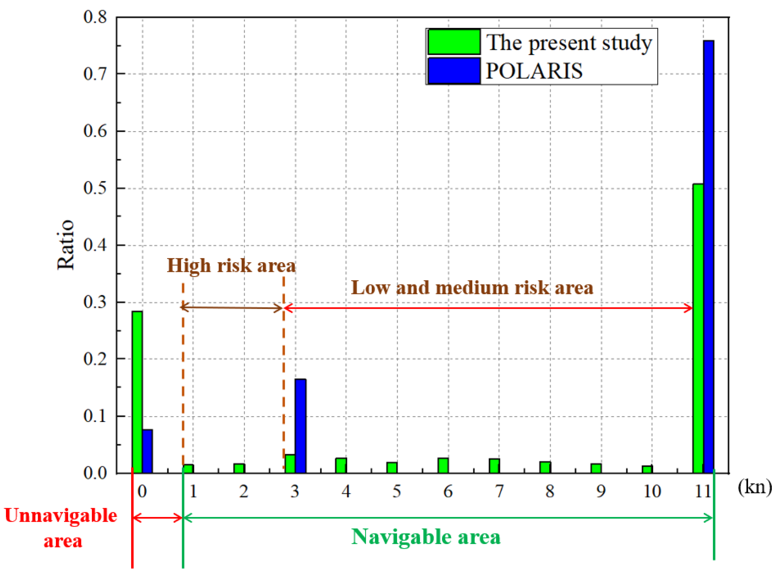
For low-risk ice areas, the recommended upper speed limit is set as the economical service speed of 11 kn.

ii.

For medium-risk areas, the speed limit by POLARIS for ice class below PC5 is used as a lower bound for ship’s advance in ice, i.e., 3.0 kn.

iii.

For high-risk areas, a minimum speed of 0.5 kn is required to keep the ship moving in ice.

iv.

For unnavigable areas, the navigation speed is less than 0.5 kn even under full engine output.

Based on the P–V model in Equation (5) and the proposed risk levels in Table 5, the relationship between RIO*, ice thickness H, and ice concentration C can be derived and expressed as follows.

$$\{\begin{array}{c}RI{O}_{\mathrm{L}}^{*}=-A\cdot \exp \left(B_{\mathrm{L}}\right)+12\\ RI{O}_{\mathrm{M}}^{*}=-3.197\ast A\cdot \exp \left(B_{\mathrm{M}}\right)-10.8698\\ RI{O}_{\mathrm{H}}^{*}=6.6445\ast A\cdot \exp \left(B_{\mathrm{H}}\right)- 26.5780\end{array}$$

(6)

where the subscripts L, M and H represent low-, medium-, and high-risk levels, respectively. The solutions for coefficient B under different risk levels are presented in Equation (7). Figure 8 displays the boundaries of the ice conditions for different risk levels using a colour map.

$$\{\begin{array}{l}{B}_{\mathrm{L}}=-0.1771\exp \left(0.6386\pi \cdot H\cdot C\right)+1.2441\exp \left[{\left(-1.51C\right)}^3\right]+1.7413\\ B_{\mathrm{M}}=-0.0483\exp \left(0.6386\pi \cdot H\cdot C\right)+0.3393\exp \left[{\left(-1.51C\right)}^3\right]+0.4749\\ B_{\mathrm{H}}=-0.0081\exp \left(0.6386\pi \cdot H\cdot C\right)+0.0566\exp \left[{\left(-1.51C\right)}^3\right]+0.0792\end{array}$$

(7)

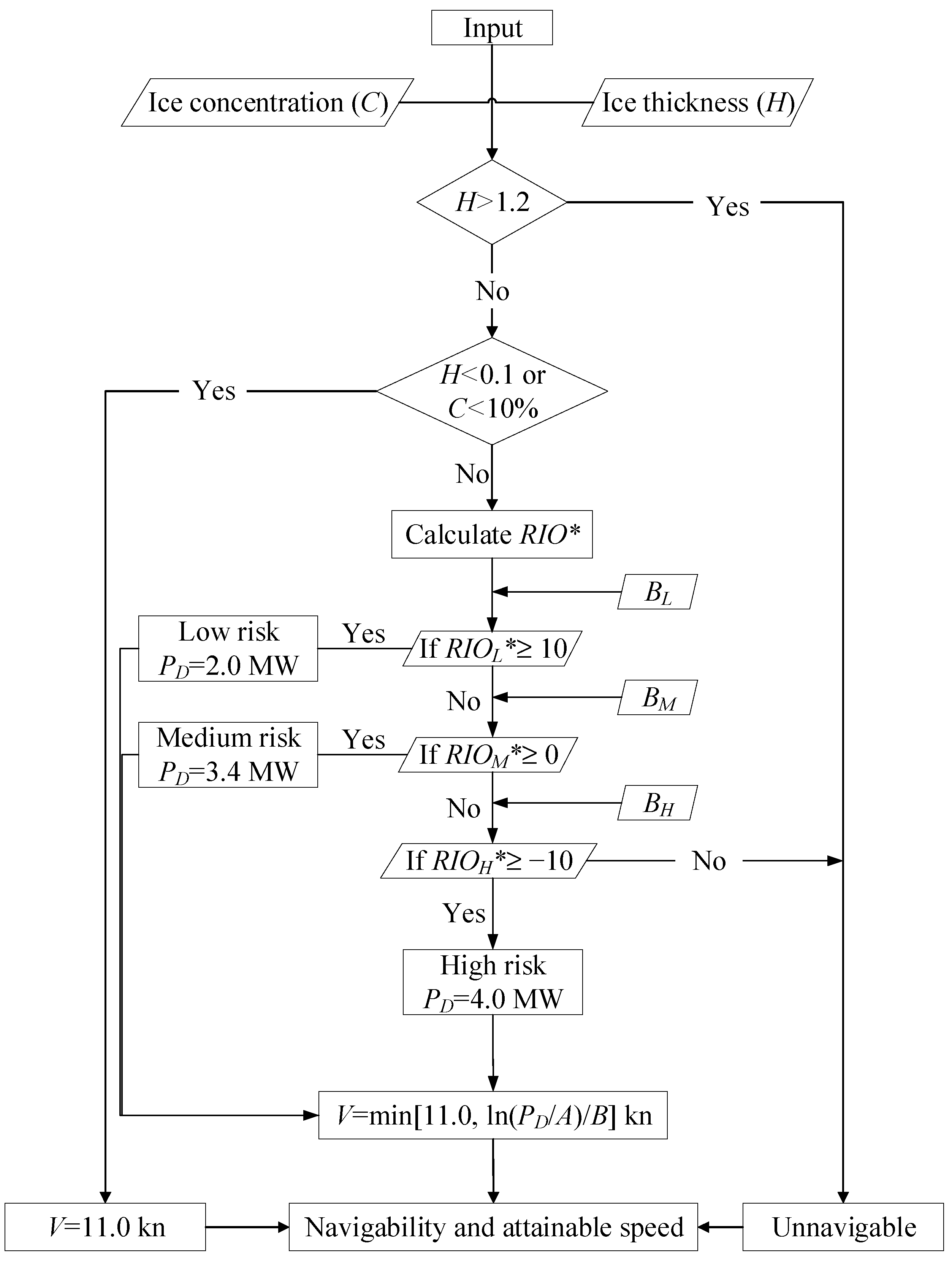
3.3. Speed Design for Various Ice Conditions

Considering the limited test data for extrapolation of the P–V relations and possible deviation of the fitted calculation model near the upper or lower bounds, it is important to define reasonable limits for the application of the proposed calculation model. For the lower bound, ice thickness levels under 0.1 m or ice concentrations less than 10% are regarded as low-risk areas, where the present ship can navigate at the economic service speed of 11 kn. For the upper bound, areas with ice thickness exceeding 1.2 m are classified as “unnavigable”, which is consistent with the POLARIS defining a zero RIV for PC6 ice class under “Medium First Year Ice” conditions. Therefore, the speed design for various ice conditions is expressed by Equation (8) according to the proposed P–V relations and the limitations.

$$\{\begin{array}{ll}V=11.0\hfill & H<{0.1}_{}|C<10\%\hfill \\ V\left(H,C,P_{\mathrm{D}}\right)=\frac{\ln \left(P_{\mathrm{D}}/A\right)}{B}\hfill & 0.1\le H\le 1.2\hfill \\ Unnavigable\hfill & H>1.2\hfill \end{array}$$

(8)

Figure 9 displays a speed matrix produced by Equation (8) using a colour map, which illustrates a direct relation between ice thickness, concentration, and ship velocity. The procedure for this speed design is shown in Figure 10 and has been used for the route planning of the present ship described in the next section.

4. Route Planning: Simulation and Case Study

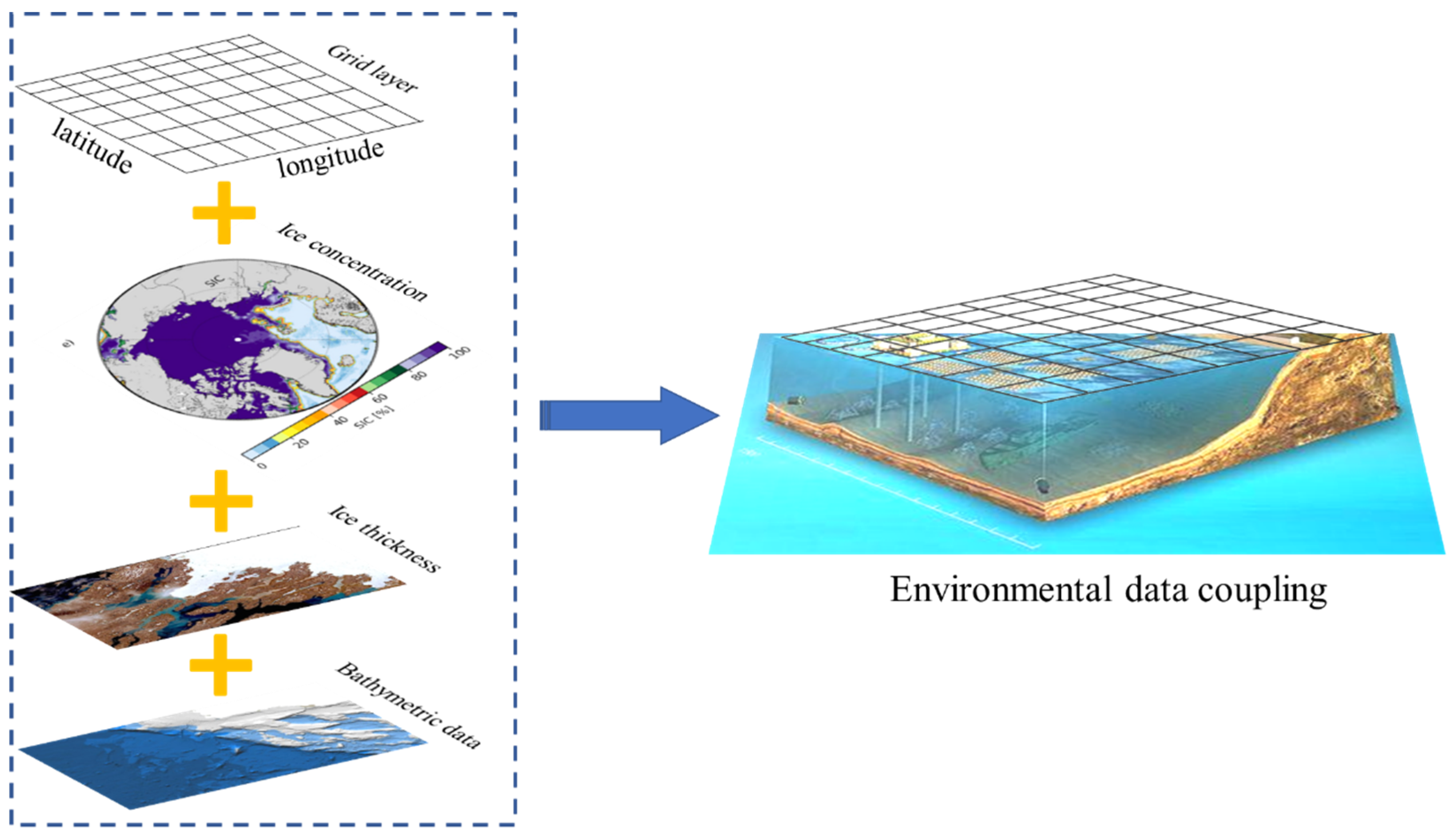
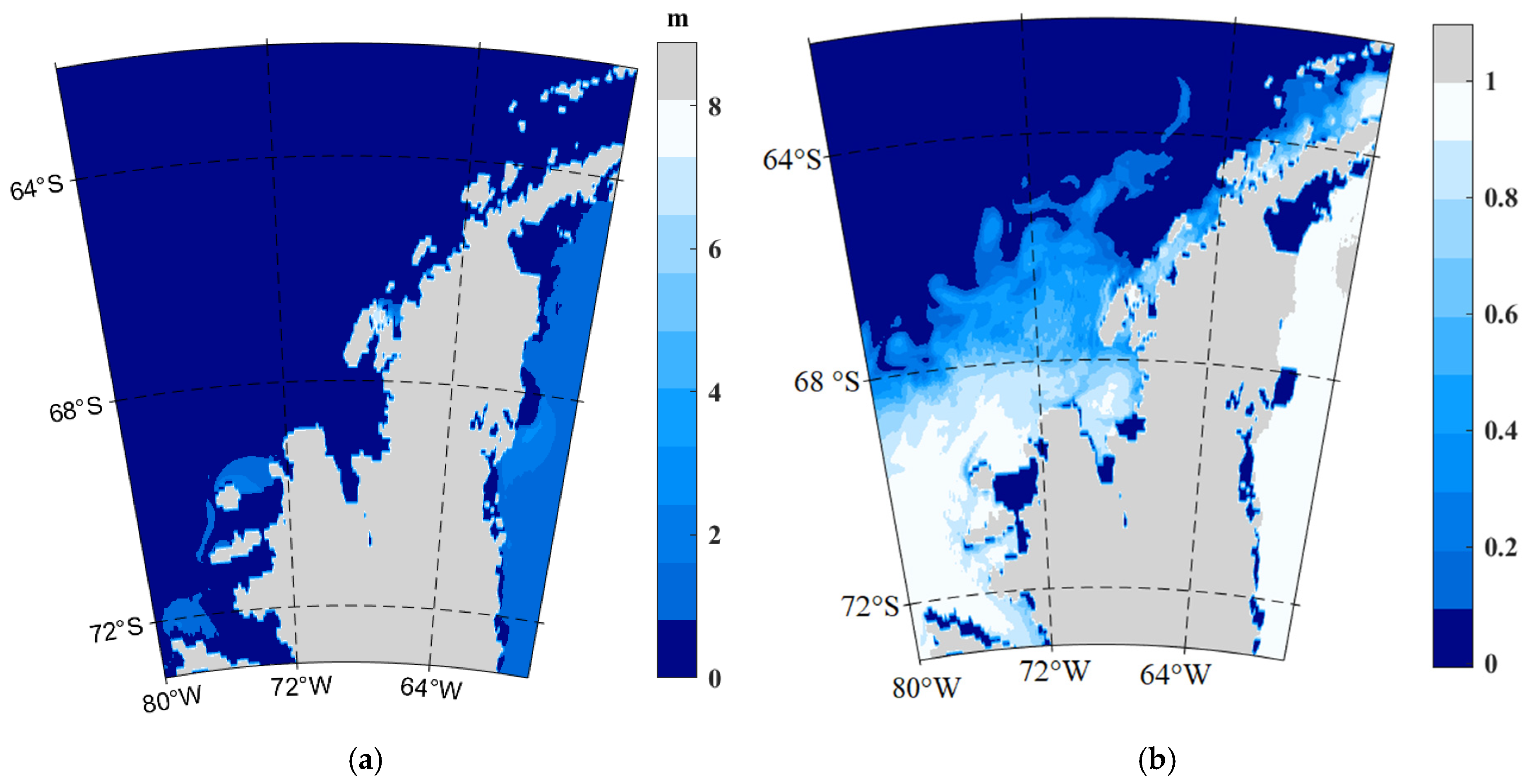
4.1. Environment Data and Design variables

In this section, a route planning simulation using the A* algorithm is performed. Detailed explanations of this algorithm can be found in [30,31,32,33,34]. The environmental data used for risk assessment and route planning include ice thickness, ice concentration, and water depth.

Table 6. Format of the input parameters of the environmental data.

Parameter	Data Source	Resolution	Format
Ice thickness Ice concentration	doi.org/10.48670/moi-00016	0.083° × 0.083° (1/12)	.NetCDF
Water depth	https://download.gebco.net/	0.0042° × 0.0042° (1/240)

lists the resolution and data formats of these input parameters from [35,36]. To address the difference in the resolution between sea ice data and water depth data, bilinear interpolations are applied to the low-resolution maps to match the high-resolution ones.

In the present route planning simulation, the environmental data has been converted to grid-based layers with reference to the longitude and latitude, as illustrated in Figure 11. Then, the navigability information can be derived using the proposed procedure in Figure 10 and expressed by:

$$I(lo{n}_i,la{t}_i)=\{Dept{h}_i,H_i,C_i\}$$

(9)

where I is the navigability information of each grid, i the grid number, lon the longitude, lat the latitude, Depth the water depth including land altitude, H the ice thickness, and C the ice concertation. The role of water depth in the risk assessment is considered to avoid grounding. The safe limit is primarily determined by the ship’s draught and under-keel clearance (UKC); the latter takes into account several factors, such as the impact of shallow waters and potential measurement inaccuracies. Additionally, it is worth noting that heave motions are more likely to occur at lower water depths, especially when the depth is less than 2.5 times the ship’s draught [37,38]. Therefore, to ensure the safety and the comfort of passengers onboard, the lower bound of the water depth is taken as 13.875 m for the present ship.

4.2. Objective Function and Constrains

Safety and efficiency are the primary objectives in the route planning in ice, which can be quantified as the shortest transit time between the starting and end points expressed by:

$$t={\displaystyle \sum _{i=1}^n\frac{L_g(site(i+1),site(i))}{V(site(i+1),site(i))}}$$

(10)

where t is the total transit time; site(i) is the location function of the ship described as site(lon_i, lat_i); V is the ship velocity from site(i) to the site(i + 1) calculated by the proposed procedure in Figure 10; L_g is the actual geographical distance from site(i) to the site(i + 1). Note that the objective function has integrated the influence of sea ice on the navigational risk, rather than relying on the shortest distance only. For safety concerns, the optimized route should satisfy several constraints, which has been mentioned above and summarized as follows:

i.

The water depth should be at least 13.875 m to ensure safety and comfort;

ii.

The ice thickness should not exceed 1.2 m for the present PC6 classed ship;

iii.

The calculated new risk index RIO* should not be lower than −10 to prevent potential besetting incidents.

4.3. Case Study

For case study, a sightseeing route that begins at the Chinese Great Wall Station in Antarctica and ends at Smyley Island is introduced, passing through five Antarctic tourist attractions with unique sceneries (see

Table 7. Route information including the locations for different stations.

No.	Station	Location	Main Scenery	Range
1	Antarctic Great Wall Station	[62.21° S, 58.95° W]	Chinese first scientific research station in the Antarctic	80°−58° W 73°−62° S
2	Anvers Island	[64.54° S, 63.45° W]	Whales
3	Renaud Island	[65.70° S, 65.97° W]	Adélies penguin
4	Adelaide Island	[67.05° S, 68.20° W]	Glaciers
5	Smyley Island	[72.60° S, 78.26° W]	Emperor penguin

). To evaluate the transit distance and time, simulations are conducted using historical daily sea ice data. Note that the present study does not account for the stop time at these stations.

This section presents a simulation-based analysis of a navigation route using daily historical sea ice data from 1 January 2021 to 31 December 2022. Environmental information is sourced from the websites mentioned above for the corresponding geographic range and date, as listed in Table 7. The route planning results based on the daily data are presented in Figure 12, with each layer representing the sea ice concentration data for each day. The varying speeds of the planned route are depicted using different colours in the image, with the colour bar for speed at the top. The land is represented by grey areas.

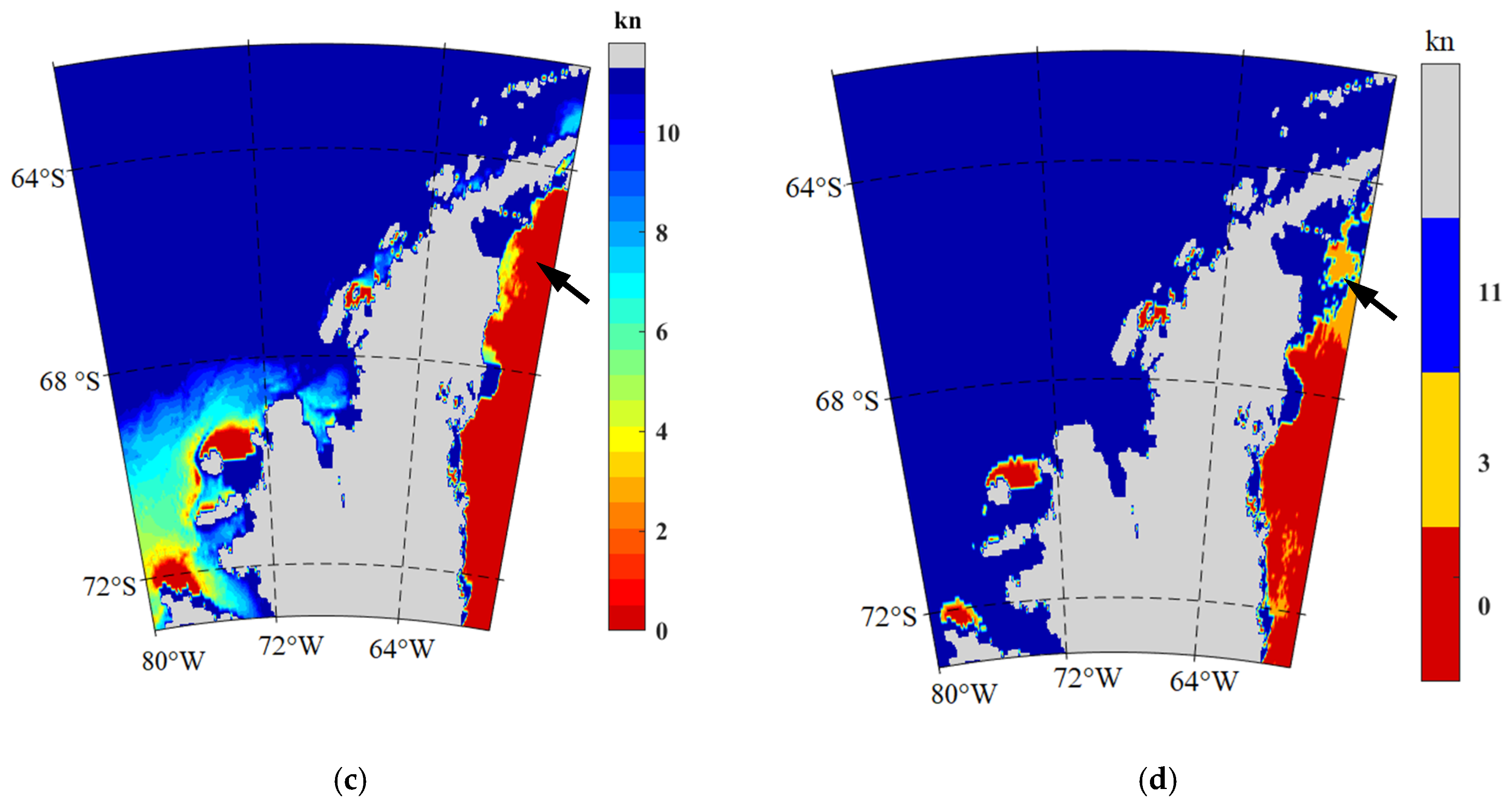
4.3.1. Speed Information Compared with POLARIS

The distribution of sea ice thickness and concentration on 17 August 2021 is shown in Figure 13a,b, respectively. Figure 13c,d display the navigability information maps obtained based on the proposed procedure by this paper and the POLARIS, respectively. The selected ice data for the analysis are characterized by varying spatial distributions, making it clearer to display the differences in the results by the two methods mentioned above.

The navigability map produced by the POLARIS offers limited information as it only includes three discontinuous speed levels: normal operation with the economic service speed of 11 kn (plotted in blue), elevated-risk operation with a recommended speed limit of 3 kn for ice class below PC5 (in yellow), and operations subject to special consideration with zero speed that should be avoided in route planning (in red). Such an approach fails to provide a continuous and detailed speed design for different ice thicknesses and concentrations. Moreover, it does not consider the propulsion capability of the ship and may lead to hazardous situations. As marked in Figure 13c,d by arrows, areas with nearly zero speeds classified by the proposed procedure of the present study are however treated as elevated-risk areas that can navigate at a speed of 3 kn. In contrast, the present method overcomes the limitations of the POLARIS by providing detailed and reliable navigability information to the operators, thereby offering a more accurate risk assessment under varying ice conditions. Figure 14 presents the ratios of different speed areas to the whole evaluated area produced by the present procedure and the POLARIS, respectively. As can be seen, about 29% of the total area is identified as “unnavigable” by the present procedure, while only 8% is detected by the POLARIS. Therefore, the proposed procedure by the present study is used for further analyses hereinafter.

4.3.2. Result Analysis and Potential Routes

Figure 15 illustrates the daily changes in the transit distance and time for the aforementioned route of Table 7 in the years 2021 and 2022, accompanied by the maximum, minimum, and average speeds for the whole trip. The visualization of the route planning is demonstrated for three different starting dates, including 2 March, 2 July, and 31 October 2021. It is noteworthy that the evaluated area in the Antarctic generally experiences a mild ice condition, with severe ice coverages mainly located south of 67° S and for a short period. The present study has analyzed the seasonal variations in this route and proposed several suggestions for the route planning in the ice based on the fluctuations in total distance, time, and speed.

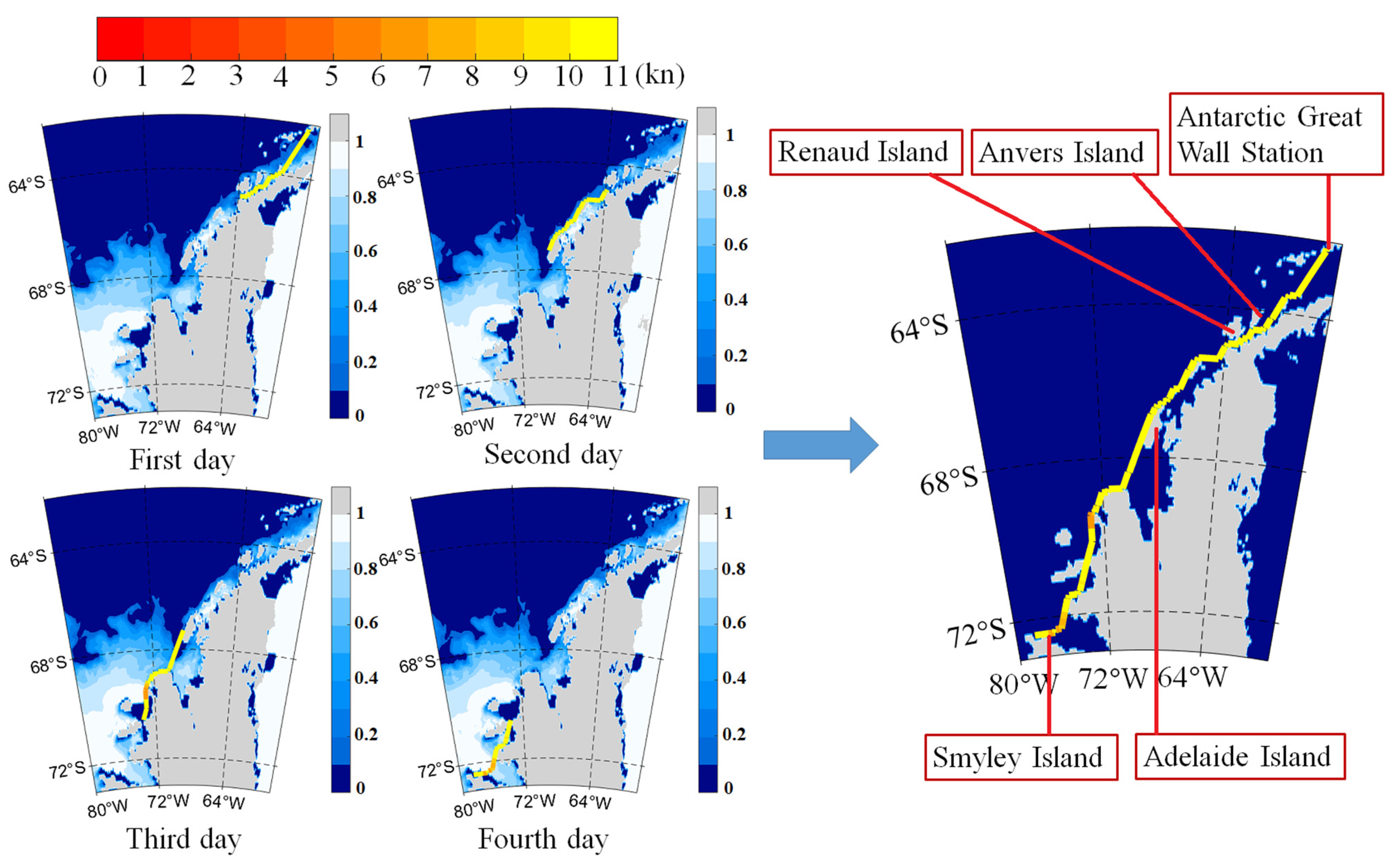
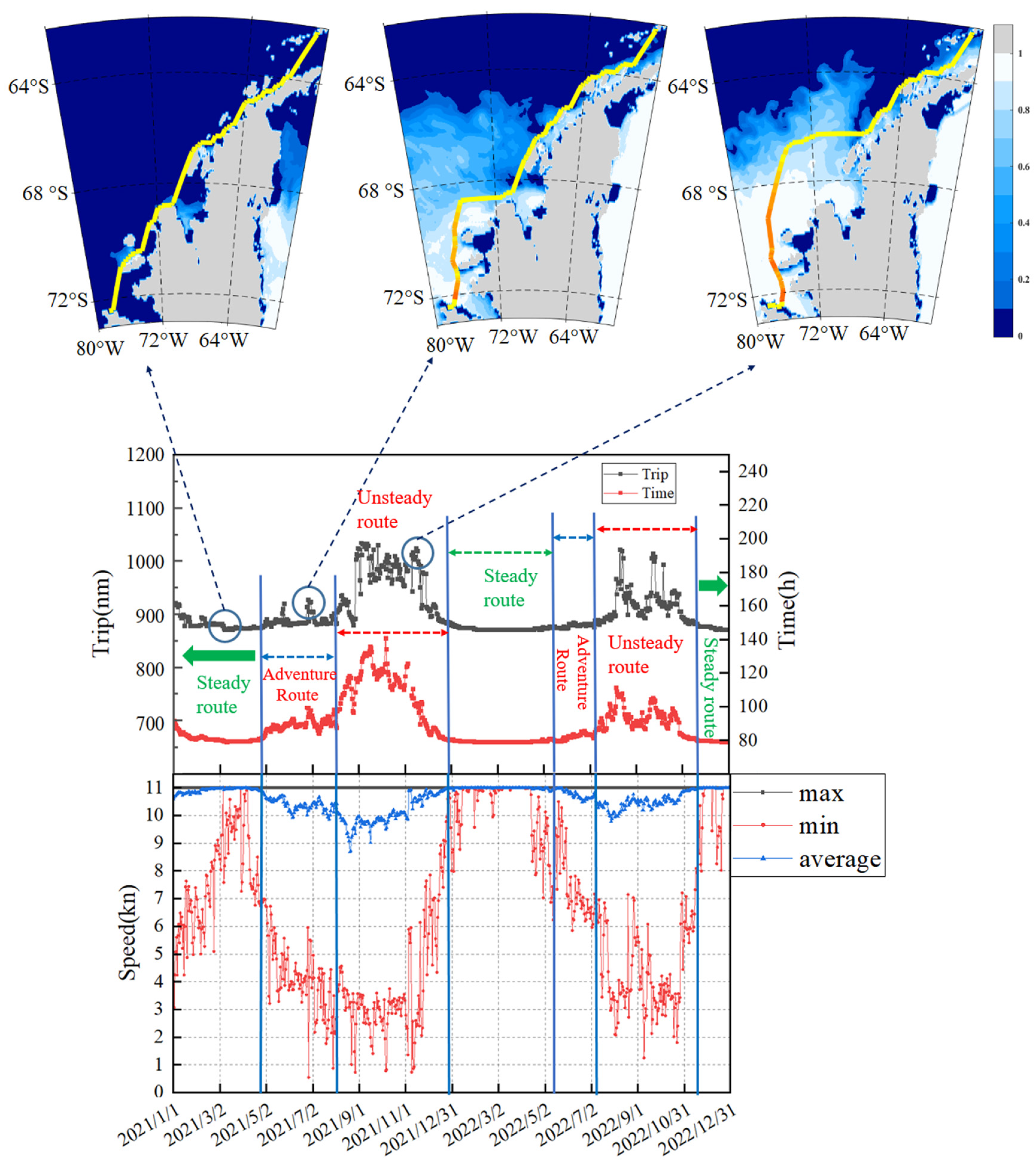
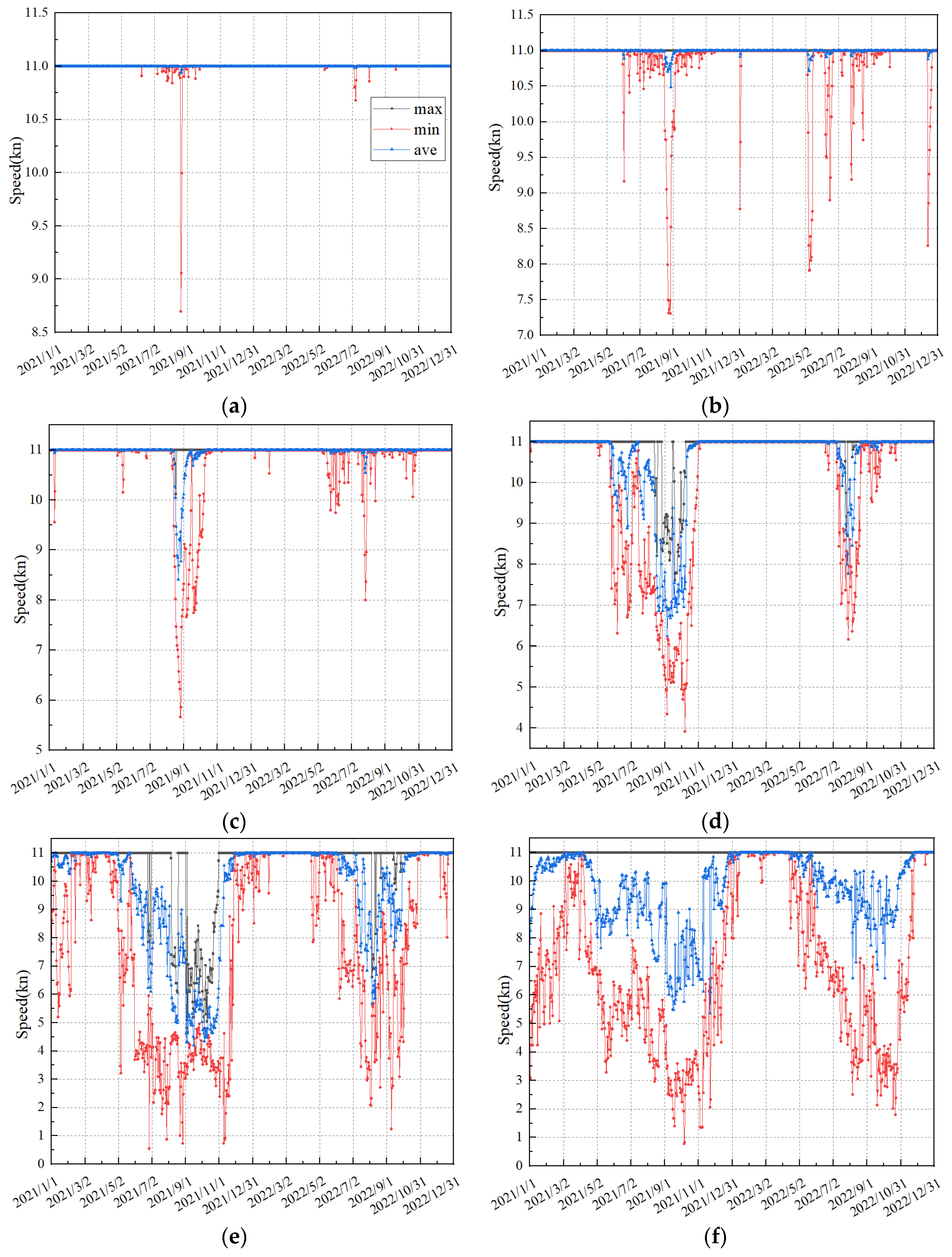
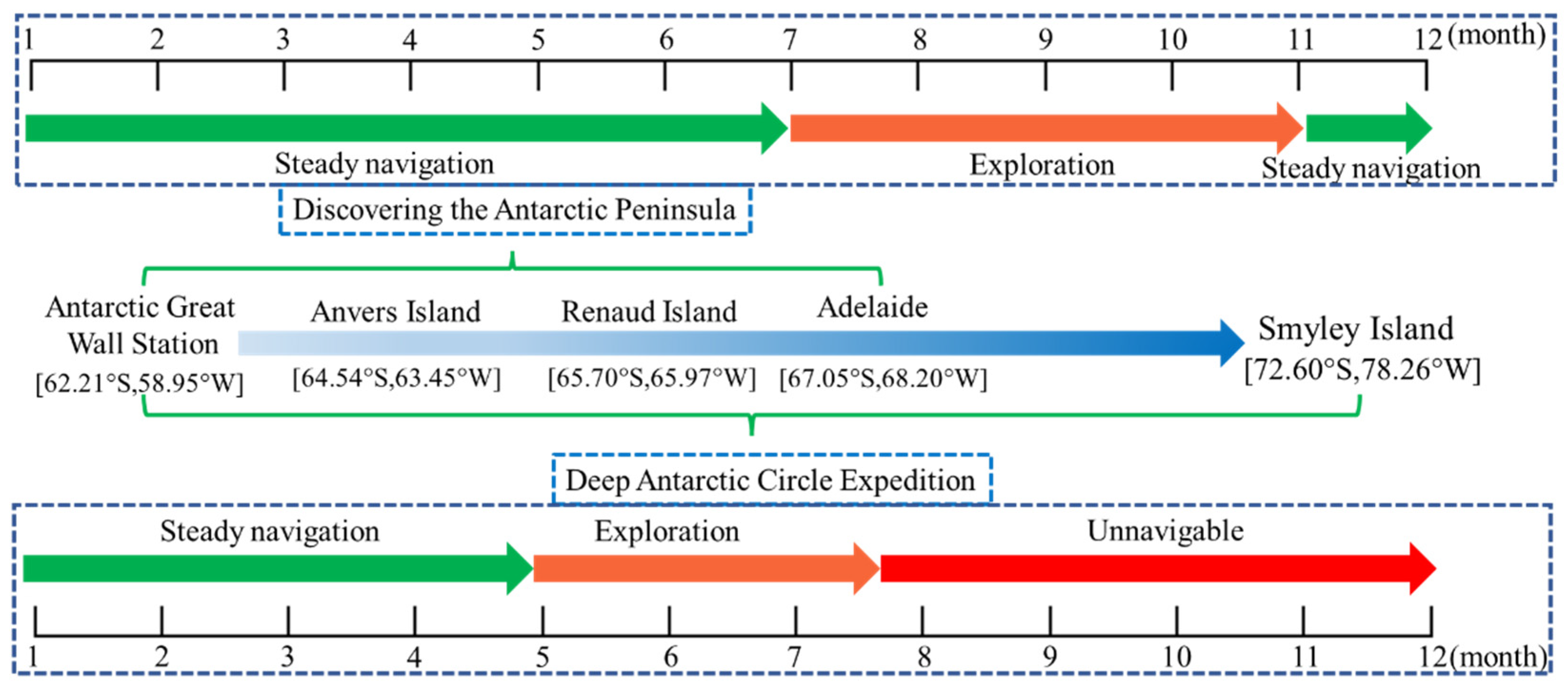
• Three navigational windows characterized by a steady state of the trip or time are identified, including 1 January to 28 April 2021, 29 December 2021 to 4 May 2022 (summer), and 22 November to 31 December 2022. These periods can provide relatively steady navigational speeds and predictable transit time for the present polar cruise ship. Additionally, these periods may offer opportunities for shore excursions and exploration of the shore ice and iceberg landscapes, as the planned route is close to the land (see Figure 15). Note that the steady period in 2022 is slightly longer than that in 2021, possibly due to the changes in sea ice conditions resulting from global warming.
• Navigational windows of minor fluctuations occur between 29 April and 2 August 2021, and between 5 May and 4 July 2022 (autumn), requiring an average speed of approximately 10.5 kn. In the south of 67° S, the speed significantly decreases, dropping to as low as 0.5 kn in some areas. As the Antarctic temperature decreases, sea ice near the land in the south of 67° S becomes thicker and denser, leading to an increase in total voyage distance and time and deviating the route from the coast. In 2021, the speed for some areas was lower than 4 kn, while in 2022, the speed was generally over 5 kn, with most regions located in the low-risk zone. These unique features make this period ideal for explorers. Nevertheless, cruise companies must consider carefully while developing routes during this window period.
• Periods from 3 August to 28 December 2021, and from 5 July to 21 November 2022 (winter and spring) are considered unsuitable for commercial navigations due to the continuous drop in temperature of coastal sea ice. Although the route in the north of 67°S has minor fluctuations, allowing access to several stations, the route in southern areas is characterized by a long distance from the coastline into the highly concentrated ice and lower attainable speeds, leading to high power requirements and fuel consumptions for the ship.

When focusing on the speed data, a gradual reduction with increasing latitude can be observed. To assess the feasibility of the present ship navigating across different latitudes, the whole area is divided into six segments by latitude boundaries. Figure 16 illustrates the minimum, maximum, and average speeds within each segment. The average speed is more than 5 kn for the whole year in the areas ranging from 62.21° S to 67.01° S, which indicates a low-risk state. Navigation within this range is feasible throughout the year, even though there are speed fluctuations during the winter. In the south of 67.01° S, seasonal variations in ice have a significant influence on the navigation speed. For the range from 67.01° S to 68.61° S, the average speed sharply declines to 4 to 7 kn during the winter, while remaining at approximately 11 kn for other periods. For the range of 68.61°−70.21° S, the average speed is consistently around the economic navigation speed from early December to May, but drops to around 4 kn during the winter. For the areas between 70.21° S and 72.6° S, navigation can be viable from January to May, with an average speed of around 10 kn and a minimum speed above 3 kn, which falls within the low-risk range. For other periods, the average speed fluctuates considerably with the minimum speed slightly lower than 1 kn.

Combining the analysis with the rules established by the polar cruise company, a long voyage can be divided into various categories, such as complete and sectional routes. Herein, a multi-level tourist route based on the voyage distance, speed, and level of risk is proposed. The final route planning and navigational windows are illustrated in Figure 17, which consist of two sections: “Discovering the Antarctic Peninsula” and “Deep Antarctic Circle Expedition”. The former includes the four locations listed in Table 7 and travels through the region between 62.21° S and 67.01° S, which is accessible year-round, including both periods of the steady navigation (January to July, November to December) and the exploration window. The “Deep Antarctic Circle Expedition” includes all the sites and extends to the high-latitude region of the Antarctic Circle, providing a more explorative experience than the “Discovering the Antarctic Peninsula” route. This route can be traversed from January to mid-July each year, with the majority of the year being open to navigation. Depending on the speed of the voyage, this route can be divided into a steady navigation period (January to May) and an expedition window (May to July).

5. Conclusions

This paper proposes an approach to predicting the propulsion performance of a PC6 classed polar cruise ship in ice based on model tests in an ice tank, and a new risk index outcome (RIO*) after the POLARIS to link the navigational risk levels to the ship’s propulsion power. On these bases, a procedure is proposed for calculating the attainable safe speeds under different risk levels corresponding to various ice conditions and then used for the speed design in the route planning of the present ship. The following conclusions can be drawn from the present study.

First of all, exponential function can be used to express the P–V relation of the present ship in pack ice conditions. After proper upper and lower bounds are defined, a continuous description on the P–V relation can be obtained based on the extrapolation of limited test data.

Secondly, four risk levels, including low, medium, high, and unnavigable, are classified with the required propulsion power in ice being 50%, 85%, 100% and >100% of the rated power, respectively. The recommended speed limit for each risk level is proposed based on the economical service speed of 11 kn, the operational limit of 3 kn by POLARIS and the minimum speed of 0.5 kn to avoid besetting, respectively. Together with the POLARIS, the speed design for the route planning under various ice conditions can be performed.

Thirdly, the simulation results show that the proposed procedure in this paper can provide more reliable and reasonable navigability information compared to the POLARIS. The identified “unnavigable” area by the present procedure accounts for 29% of the simulated area, while only 8% is detected by POLARIS.

Finally, as a case study, potential routes in the Antarctic region for the present ship are introduced, i.e., “Deep Antarctic Circle Expedition” and “Discovering the Antarctic Peninsula”, based on the analyses of the simulation results especially regarding the fluctuations of the average speed, which can provide reference for the polar cruise industry. Note that the proposed routes are based on the simulation using historical sea ice data. Considering the effect of global warming, the navigational windows may extend both spatially and temporally.

The approach and procedure presented in this paper are only effective for the present polar cruise ship. Nevertheless, the idea of using propulsion performance in ice to determine the risk levels and speed design in route planning under various ice conditions can be adopted to other ships. The route planning of the present study only considers the variation in the ice conditions from a “global” spatial scale. For the navigation in ice, the possible inclusions of multi-year ice, ice ridges, growlers or bergy bits at a “local” spatial scale can bring critical threats to the ship, where the ship’s structural response (e.g., deformation of the hull plate), maneuverability (e.g., turning circle), and operability (e.g., roll amplitude, accelerations) can govern the determination of attainable speeds instead of the propulsion power itself. Therefore, ice maps of high resolution and details are essential, and it is also recommended to establish a comprehensive risk level definition based on the integrated consideration of ship’s propulsion capability, structural safety, maneuverability, and operability. If real-time sea ice data are available, real-time route planning can also be achieved by, e.g., the combined simulation of pathfinding and ship maneuvering, which will be addressed in future studies.

References

1. Wang, S.; Mu, Y.; Zhang, X.; Xie, J. Polar tourism and environment change: Opportunity, impact and adaptation. Polar Sci. 2020, 25, 100544. [Google Scholar]
2. IAATO. Antarctic Tourism Statistics, 1992–2019. Available online: http://www.iaato.org/ (accessed on 25 May 2023).
3. Shepherd, A.; Fricker, H.; Farrell, S. Trends and connections across the Antarctic cryosphere. Nature 2018, 558, 223–232. [Google Scholar] [CrossRef]
4. AECO. The Association of Arctic Expedition Cruise Operators. 2022. Available online: https://www.aeco.no (accessed on 25 May 2023).
5. Lavissière, A.; Sohier, R.; Lavissière, M.C. Transportation systems in the Arctic: A systematic literature review using textometry. Transp. Res. Part A 2020, 141, 130–146. [Google Scholar] [CrossRef]
6. Krivoguz, D.; Nosova, E.; Piatinskii, M. Analysis of spatio-temporal changes in Arctic Ocean ecosystem using machine learning and its impact on marine transportation system. Transp. Res. Procedia 2022, 63, 2967–2971. [Google Scholar] [CrossRef]
7. Montewka, J.; Goerlandt, F.; Lensu, M.; Kuuliala, L.; Guinness, R. Toward a hybrid model of ship performance in ice suitable for route planning purpose. J. Risk Reliab. 2019, 233, 18–34. [Google Scholar] [CrossRef]
8. Khan, B.; Khan, F.; Veitch, B.; Yang, M. An operational risk analysis tool to analyze marine transportation in Arctic waters. Reliab. Eng. Syst. Saf. 2018, 169, 485–502. [Google Scholar] [CrossRef]
9. Li, Z.; Ringsberg, J.; Rita, F. A voyage planning tool for ships sailing between Europe and Asia via the Arctic. Ships Offshore Struc. 2020, 15, 10–19. [Google Scholar] [CrossRef]
10. Wang, Y.; Liu, K.; Zhang, R.; Qian, L.; Shan, Y. Feasibility of the Northeast Passage: The role of vessel speed, route planning, and icebreaking assistance determined by sea-ice conditions for the container shipping market during 2020–2030. Transp. Res. Part E 2021, 149, 102235. [Google Scholar] [CrossRef]
11. Lee, H.; Roh, M.; Kim, K. Ship route planning in Arctic Ocean based on POLARIS. Ocean Eng. 2021, 234, 109297. [Google Scholar] [CrossRef]
12. IMO. MSC.1-Circ.1519—Guidance on Methodologies for Assessing Operational Capabilities and Limitations in Ice; IMO: London, UK, 2016. [Google Scholar]
13. Browne, T.; Tran, T.; Veitch, B.; Smith, D.; Khan, F. A method for evaluating operational implications of regulatory constraints on Arctic shipping. Mar. Policy 2022, 135, 104839. [Google Scholar] [CrossRef]
14. Lee, S. A Study on the Method of Simultaneous Determination of Path and Speed for Ship Route Planning. Ph.D. Thesis, Seoul National University, Seoul, Republic of Korea, 2017. [Google Scholar]
15. Kotovirta, V.; Jalonen, R.; Axell, L.; Riska, K.; Berglund, R. A system for route optimization in ice-covered waters. Cold Reg. Sci. Technol. 2009, 55, 52–62. [Google Scholar] [CrossRef]
16. Choi, M.; Chuang, H.; Yamaguchi, H.; Nagakawa, K. Arctic sea route path planning based on an uncertain ice prediction model. Cold Reg. Sci. Technol. 2015, 109, 61–69. [Google Scholar] [CrossRef]
17. Zhang, C.; Zhang, D.; Zhang, M.; Mao, W. Data-driven ship energy efficiency analysis and optimization model for route planning in ice-covered Arctic waters. Ocean Eng. 2019, 186, 106071. [Google Scholar] [CrossRef]
18. FSICR. Ice Class Regulations and the Application Thereof (Finnish-Swedish Ice Class Rules); Finnish Transport Safety Agency (TRAFI): Helsinki, Finland, 2017. [Google Scholar]
19. ISO 19906; Petroleum and Natural Gas Industries—Arctic Offshore Structures. International Organization for Standardization: Geneva, Switzerland, 2019.
20. ITTC. Propulsions Test in Ice. In ITTC Recommended Procedures and Guidelines; ITTC: Zurich, Switzerland, 2021. [Google Scholar]
21. Huang, Y. Model test study of the nonsimultaneous failure of ice before wide conical structures. Cold Reg. Sci. Technol. 2010, 63, 87–96. [Google Scholar] [CrossRef]
22. Sun, J.; Huang, Y. Investigations on the ship-ice impact: Part 1. Experimental methodologies. Mar Struct. 2020, 72, 102772. [Google Scholar] [CrossRef]
23. Timco, G.; Weeks, W. A review of the engineering properties of sea ice. Cold Reg. Sci. Technol. 2010, 60, 107–129. [Google Scholar] [CrossRef]
24. Li, Z.; Marcel, N.; Takenobu, T.; Christian, H. Analysis on the crystals of sea ice cores derived from Weddell Sea, Antarctica. Chin. J. Polar Res. 2009, 21, 177–185. [Google Scholar]
25. Timco, G. Ice forces on structures: Physical modeling techniques. In Proceedings of the IAHR Symposium on Ice, Hamburg, Germany, 27–31 August 1984; Volume 4, pp. 117–150. [Google Scholar]
26. ITTC. General Guidance and Introduction to Ice Model Testing. In ITTC Recommended Procedures and Guidelines; ITTC: Zurich, Switzerland, 2021. [Google Scholar]
27. ITTC. Guidelines for Modelling of Complex Ice Environments. In ITTC Recommended Procedures and Guidelines; ITTC: Zurich, Switzerland, 2021. [Google Scholar]
28. ITTC. Resistance Test in Ice. In ITTC Recommended Procedures and Guidelines; ITTC: Zurich, Switzerland, 2021. [Google Scholar]
29. MAN Diesel & Turbo. SFOC Optimisation Methods for MAN B&W Two-Stroke IMO Tire II Engines; MAN Diesel & Turbo: Copenhagen, Denmark, 2010. [Google Scholar]
30. Topaj, A.; Tarovik, O.; Bakharev, A.; Kondratenko, A. Optimal ice routing of a ship with icebreaker assistance. Appl. Ocean Res. 2019, 86, 177–187. [Google Scholar] [CrossRef]
31. Zvyagina, T.; Zvyagin, P. A model of multi-objective route optimization for a vessel in drifting ice. Reliab. Eng. Syst. Safe 2022, 218, 108147. [Google Scholar] [CrossRef]
32. Lehtola, V.; Montewka, J.; Goerlandt, F.; Guinness, R.; Lensu, M. Finding safe and efficient shipping routes in ice-covered waters: A framework and a model. Cold Reg. Sci. Technol. 2019, 165, 102795. [Google Scholar] [CrossRef]
33. Wang, Y.; Zhang, R.; Qian, L. An improved A* algorithm based on hesitant fuzzy set theory for multi-criteria Arctic route planning. Symmetry 2018, 10, 765. [Google Scholar] [CrossRef]
34. Li, Z.; Yao, C.; Zhu, X.; Gao, G.; Hu, S. A decision support model for ship navigation in Arctic waters based on dynamic risk assessment. Ocean Eng. 2022, 244, 110427. [Google Scholar] [CrossRef]
35. General Bathymetric Chart of the Oceans (GEBCO). GEBCO Gridded Bathymetry Data Download. Available online: https://download.gebco.net/ (accessed on 6 May 2023).
36. Copernicus Marine Environment Monitoring Service. Global Ocean Physics Analysis and Forecast. Available online: https://data.marine.copernicus.eu/product/GLOBAL_ANALYSISFORECAST_PHY_001_024/download?dataset=cmems_mod_glo_phy_anfc_0.083deg_P1D-m (accessed on 6 May 2023).
37. Briggs, M. Ship Squat Predictions for Ship/Tow Simulator; ERDC/CHL CHETN-I-72; US Army Corps of Engineers: Washington, DC, USA, 2006. [Google Scholar]
38. Jachowski, J. Assessment of ship squat in shallow water using CFD. Arch. Civ. Mech. Eng. 2008, 8, 27–36. [Google Scholar] [CrossRef]
Figure 1. The model ship used for the propulsion tests.
Jmse 11 01655 g001
Figure 2. Section picture of the model ice.
Jmse 11 01655 g002
Figure 3. Ship–ice interaction scenarios under different ice concentrations: (a) ice floes rebounding away from the ship under 50% ice concentration; (b) ice bending failure under 90% ice concentration. The yellow solid lines outline the ice floes that interact with the model ship. The red arrows illustrate the trajectories of the ice floes after rebounding away, and the red dotted lines illustrate the bending failure of the floe’s edge.
Jmse 11 01655 g003
Figure 4. Time series of the measured data in model scale including the ship velocity (V), propeller rate (n), shaft thrust (T), shaft torque (Q), and towing force (Pull).
Jmse 11 01655 g004
Figure 5. The relationship between required shaft power and ship velocity under tested ice conditions in full scale. Least squares method is used to provide the best fit according to Equation (4). (a) H = 1.0 m; (b) H = 0.5 m.
Jmse 11 01655 g005
Figure 6. PV curve groups after extrapolation to other ice conditions based on the tested data. (a) H = 1.0 m; (b) H = 0.5 m.
Jmse 11 01655 g006
Figure 7. The fitted surfaces of A and B for the PV relation as functions of ice thickness H and concentration C.
Jmse 11 01655 g007
Figure 8. Risk levels identification under different ice conditions based on RIO*.
Jmse 11 01655 g008
Figure 9. Speed matrix under different ice thickness H and concentration C plotted by a colormap. The dark area indicates “unnavigable” conditions.
Jmse 11 01655 g009
Figure 10. Procedure to calculate the attainable speed based on RIO* and P-V relation.
Jmse 11 01655 g010
Figure 11. Environmental input data coupling of ice thickness, ice concentration, and water depth data based on latitude and longitude coordinates.
Jmse 11 01655 g011
Figure 12. Example of route planning from Antarctic Great Wall Station to Smyley Island based on daily environmental data. The color-bar represents different navigation speeds.
Jmse 11 01655 g012
Figure 13. (a) spatial distribution of ice thickness on 17 August 2021; (b) spatial distribution of ice concentration on 17 August 2021; (c) ship velocity map calculated by the proposed procedure of this paper; (d) ship velocity map calculated by POLARIS.
Jmse 11 01655 g013aJmse 11 01655 g013b
Figure 14. Proportion of navigation speeds produced by the present procedure (green bar) and the POLARIS (blue bar).
Jmse 11 01655 g014
Figure 15. Simulated results for the transit distance, time, and speed from the start station to Smyley Island at different departure dates during the years 2021 and 2022.
Jmse 11 01655 g015
Figure 16. Simulated results of the navigation speed for different latitude intervals during the years 2021 and 2022. (a) 62.21°–63.81° S. (b) 63.81°–65.41° S. (c) 65.41°–67.01° S. (d) 67.01°–68.61° S. (e) 68.61°–70.21° S. (f) 70.21°–72.60° S.
Jmse 11 01655 g016
Figure 17. Potential routes based on the station location, navigability and period proposed by the present study.
Jmse 11 01655 g017