Abstract
Spatial wave fields around floating bodies are important for the understanding of hydrodynamics, and particularly the wave drift forces, of floating bodies in waves; however, experimental measurement of these fields is challenging. This paper presents a stereo reconstruction method for three-dimensional (3D) surface wave fields around floating bodies in a wave tank. Styrofoam markers were attached to a flexible net in a regular grid, called a marker net, and were placed on the water surface to be used as targets for stereo cameras (SCs). A thin plate spline was applied to the markers detected by the SCs to reconstruct the 3D surface wave profile around a floating body model. The proposed method was validated by measuring the wave field around a cylindrical floating body with a footing at its bottom. These experiments were conducted under regular wave incidence conditions. A wave elevation time series measured using a servo-controlled wave gauge was used as the benchmark data. The 3D surface wave field reconstruction method was applied under three different conditions: without the model, with a fixed model, and with a freely oscillating model. The results showed reliable reconstructions of the scattering and radiation waves. The marker net’s effects on the floating body’s motion and the surrounding wave fields were shown to be negligible by comparing the results acquired with and without the marker net.
Keywords:
stereo camera; marker net; tank experiment; floating body; radiation wave; scattering wave 1. Introduction
To study the hydrodynamic forces that act on ships and floating bodies, tank experiments are commonly conducted using scale models of these floating structures. Although the focus of such experiments is generally on the hydrodynamic forces, these forces are strongly related to the waves generated by the ship or the floating body. Ship wakes, i.e., the waves generated by ships moving through still water, have a direct relationship with the wave-making resistance (e.g., [1]). Radiation and scattering waves, which are generated by ships moving with a forward speed in waves, induce added resistance in waves [2,3,4,5]. For floating bodies with zero forward speed, these waves induce wave drift forces [6,7]. Therefore, measurements of the waves that are generated around ships and floating bodies have also been attempted via tank experiments.
Resistance, capacitance, and servo-controlled wave gauges have been used widely to measure wave elevations in tank experiments [8]. These gauges are accurate measurement sensors with low uncertainty, but the waves can basically only be measured at a single point. Ohkusu [3] and Kashiwagi [4] proposed a method for indirect estimation of the longitudinal profiles of the radiation and scattering waves generated by a ship model when moving at a constant speed using a single-point wave gauge or an array of such wave gauges aligned longitudinally in a tank. In addition, spatial wave profiles can be obtained by using multiple conventional single-point wave gauges and repeating the measurements after changing the positions of the wave gauges [9,10,11], but this method is very time-consuming. It is thus desirable to be able to measure the spatial wave profiles directly.
One possible solution that can enable such direct areal wave measurements is the stereo imaging technique. Spatial wave profile reconstruction using stereo cameras (SCs) has been realized successfully, particularly for waves in a real ocean or lake [12,13,14,15]. The key to realization of stereo reconstruction of the wave fields is that the air/water interface must have a diffusely reflecting surface, i.e., a Lambertian surface. The wave surface in a real ocean can be treated as a Lambertian surface because there are ripples or air bubbles on the wave surface that act as scattering substances. However, it is difficult to consider the water surface in an experimental tank to be a Lambertian surface because there are almost no such scattering substances on its surface. Although some studies have attempted to apply stereo imaging techniques to wave profile reconstruction of non-Lambertian water surfaces in tanks (e.g., [16]), it is desirable to texture the water surface to give it a Lambertian characteristic when applying stereo imaging techniques.
One example of an approach to make the water surface in a tank Lambertian is to give the surface a dusting of fine particles. For example, aluminum powder [17], ground coffee [18], and polypropylene particles [19] have all been dispersed on water surfaces for that purpose. Takahei and Inui [17] and Gomit et al. [19] successfully measured the spatial wake profiles generated by ship models in still water. Another example approach involves dying the water to a milky white color and then projecting a pattern onto the surface [20]. However, fine particle dusting and coloring of the water are usually difficult methods to implement because of the constraints of the available experimental facilities. To circumvent this difficulty, Gomit et al. [21] suggested use of laser beams to project a dot pattern onto the water surface. In this method, detection of the air/water interface is difficult because the laser beams are projected not only onto the air/water interface but also, to some extent, under the water surface. However, this method is useful for tanks in which coloration of the water or dispersion of fine particles on the water is prohibited.
Another solution for these water tank facilities is to disperse retrievable scattering objects on the water and then track the motion of the individual objects using the stereoscopic particle tracking velocimetry (PTV) technique. PTV measurements of a single freely-floating object on the surface of water enabled visualization of surface-wave particle trajectories [22,23,24]. Tracking floating objects constrained horizontally by vertically tensioned wires enabled measurement of the wave elevation at fixed points as a counterpart to conventional single-point wave gauges [25,26]. To perform areal surface-wave measurements by PTV, Houtani et al. [27] dispersed multiple floats with a diameter of approximately 20 mm. Mozumi et al. [28] also placed floats with a diameter of approximately 20 mm on water in a regular grid using a flexible net. The latter method was termed the marker net method. The spatial wave profiles of unidirectional modulated wave trains [29,30] and slanted solitons and breathers [31] were reconstructed using these methods. However, these methods have not been applied to measurement of the wave fields that occur around models of ships and floating bodies in tanks to date.
This study was originally motivated by the research and development of the bow shape of ships to reduce the added resistance in waves by Sakurada et al. [5]. The bow shape is designed to suppress the waves reflected forward from the bow for incident waves with short wavelengths compared to the ship’s length. The suppression of the reflected waves was demonstrated visually and qualitatively by images of surface wave fields around the bow. Their results showed the importance of detailed observation of the wave phenomena around ships, which is the cause of the added resistance in waves, in the development of an optimal bow shape. Quantitative measurements of spatial wave profiles around ships and floating bodies could further deepen understanding of their hydrodynamics in waves. However, as reviewed in this section, quantitative measurement of these profiles in tank experiments is challenging.
Therefore, the objective of this study is to develop an experimental method to measure the three-dimensional (3D) surface wave profiles around floating bodies. In this study, the wave field around a floating body, which consists of incident, radiation, and scattering waves, was measured using SCs in combination with a marker net. Unlike the previously proposed method for indirect spatial wave-profile estimation around a ship model [3,4], the method proposed in this study measures the spatial profiles of the waves around a floating body model directly. In addition, the proposed method makes it possible to measure waves in situations where it is difficult to install conventional wave gauges, e.g., inside the chambers of an air-cushion platform [32].
Section 2 presents the method for reconstruction of the 3D surface wave fields from target markers on the water surface as detected by the SCs. The experimental setup, including the floating body model, the SCs, and the marker net, is described in Section 3. The wave elevations around a floating body model obtained when using the proposed method are compared with wave gauge records, and examples of the reconstructed 3D surface wave profiles around the model are presented in Section 4. As a potential application of the proposed method, Section 5 presents some examples of radiation and scattering wave fields that were extracted from wave profiles measured under various model constraints. The question of whether the presence of a marker net can affect the floating body model’s motion and the ambient wave fields is also discussed. The conclusions drawn from this study follow in Section 6. Note that the terms “radiation wave” and “scattering wave” are used in this study to represent both dimensional and nondimensional wave elevations in a broad sense, although these terms must sometimes be defined in a narrower sense as the waves that are nondimensionalized by the incident wave amplitude.
2. Reconstruction of 3D Wave Fields around a Floating Body Model
The proposed measurement method is categorized as a PTV method. The 3D motions of individual target markers placed on the water surface are tracked by the SCs. In this study, a commercial motion capture system, Qualisys (Qualisys AB, Göteborg, Sweden), was used to provide the SCs. The Qualisys system outputs the 3D coordinates of the markers by calibrating the SCs appropriately in advance (see Section 3.3). This section describes the method used to reconstruct the 3D surface wave profiles from these output marker coordinates. A method to separate the scattering and radiation waves from the reconstructed wave fields under three different model conditions is also described. These conditions include measurements performed without a model, performed with a fixed model, and performed with a freely oscillating model.
2.1. Reconstruction of Wave Fields
Spatial wave fields were reconstructed from the 3D coordinates of the markers as measured using the SCs. The data of some misrecognized markers that deviated obviously from the wave surface were excluded from the analysis in advance. One of the main causes of marker misidentification was infrared light reflected from the ripples generated by the floating body model or by the marker net (Appendix A).
In each time frame, a thin plate spline (TPS) [33] was applied to the remaining markers to estimate the wave elevation at any position in the analysis zone, which will be defined later in the paper in Section 3. The TPS provides a curved surface by interpolating a data cluster with noise. The target wave surface to be estimated was expressed as a single-valued function with respect to the horizontal coordinates, where , and f was evaluated such that the following objective function G was minimized:
with
where j denotes the marker index. The minimization of corresponds to a spline surface that passes through all the markers. In contrast, the minimization of corresponds to a plane obtained from a least-squares approximation of the markers. The objective function G is then defined as the weighted sum of and , where .
A physically reasonable summation of the two terms in Equation (1), and , requires that the dimensions of and be coincident. For this requirement, x and y must be dimensionless. For convenience, x and y have been nondimensionalized here by (mm), such that the values of x and y can be treated as the raw dimensional data. The value of may affect the appropriate value of p for the TPS. In this study, was used. The minimization problem with Equations (1) and (2) was solved using the “tpaps” function provided by MATLAB [33].
As a result of the application of the TPS, the proposed method cannot handle breaking waves, which are expressed as a multi-valued function with respect to the horizontal coordinates . In addition, waves with wavelengths shorter than the marker intervals cannot be resolved within the stereo-reconstructed wave fields. These factors represent the limitations of the proposed method.
2.2. Extraction of Radiation and Scattering Waves
The wave field around a floating body oscillating in waves is composed of the incident wave , the radiation wave , and the scattering wave . Under the linear assumption, is then expressed as the sum of these component waves, i.e.:
The incident wave , the radiation wave , and the scattering wave can be separated by measuring the wave fields under differing constraint conditions for the floating body model.
In this study, the wave fields were measured under the following three conditions:
- (i)
- The model was absent (only the incident wave was measured) ();
- (ii)
- The model was fixed ();
- (iii)
- The model was allowed to heave and pitch freely ().
In case (i) without the model, the wave field was composed of the incident wave alone. In case (ii) with the fixed model, the incident wave was scattered by the model. Therefore, the wave around the model was composed of the incident and scattering waves, i.e., . In case (iii) with the oscillating model, the wave was radiated because of the motion of the model. Therefore, the wave around the model comprised the incident, scattering, and radiation waves, i.e., .
The scattering, radiation, and disturbance waves ( and , respectively) can be extracted by subtracting the wave fields that were reconstructed under the different constraint conditions, as illustrated in Table 1. However, the radiation waves extracted based on in this study include components that can be attributed to both heave and pitch motions. To measure the radiation waves that can be attributed to each degree of freedom, forced oscillation experiments must therefore be performed for each mode [3,4]. Note that in the nonlinear regime, the wave field around freely oscillating floating bodies cannot necessarily be expressed as a linear superposition of the component waves of and , as in Equation (3). In this regime, interpretation of the component wave fields that were extracted using the methods described in Table 1 is complex and is beyond the scope of this paper, but this interpretation is important from the perspective of the system’s nonlinearity, as shown in the nonlinear interactions between waves and ships [4] and between waves and ice floes [34].

Table 1.
Components comprising waves around a floating body and their extraction methods from tests –.
3. Experimental Setup
3.1. Floating Body Model and Tank
A tank experiment was conducted using a cylindrical floating body model with a footing at its bottom (Figure 1) to measure the wave fields around this model. The main properties of this model are listed in Table 2. The same model was used in previous works [35,36]. A strong nonlinearity in the model’s motion in the waves was observed and was attributed to a vortex shedding from the footing. This study used a larger displacement and a deeper draft than in the previous experiments [35,36].
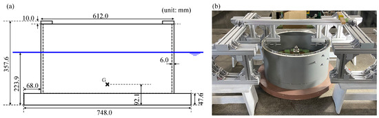
Figure 1.
Subject model of a shallow-draft cylindrical floating body with a footing. (a) Schematic side view; (b) image of the body (acquired during a swing test to evaluate the pitch radius of gyration).
Table 2.
Main properties of the floating body model.
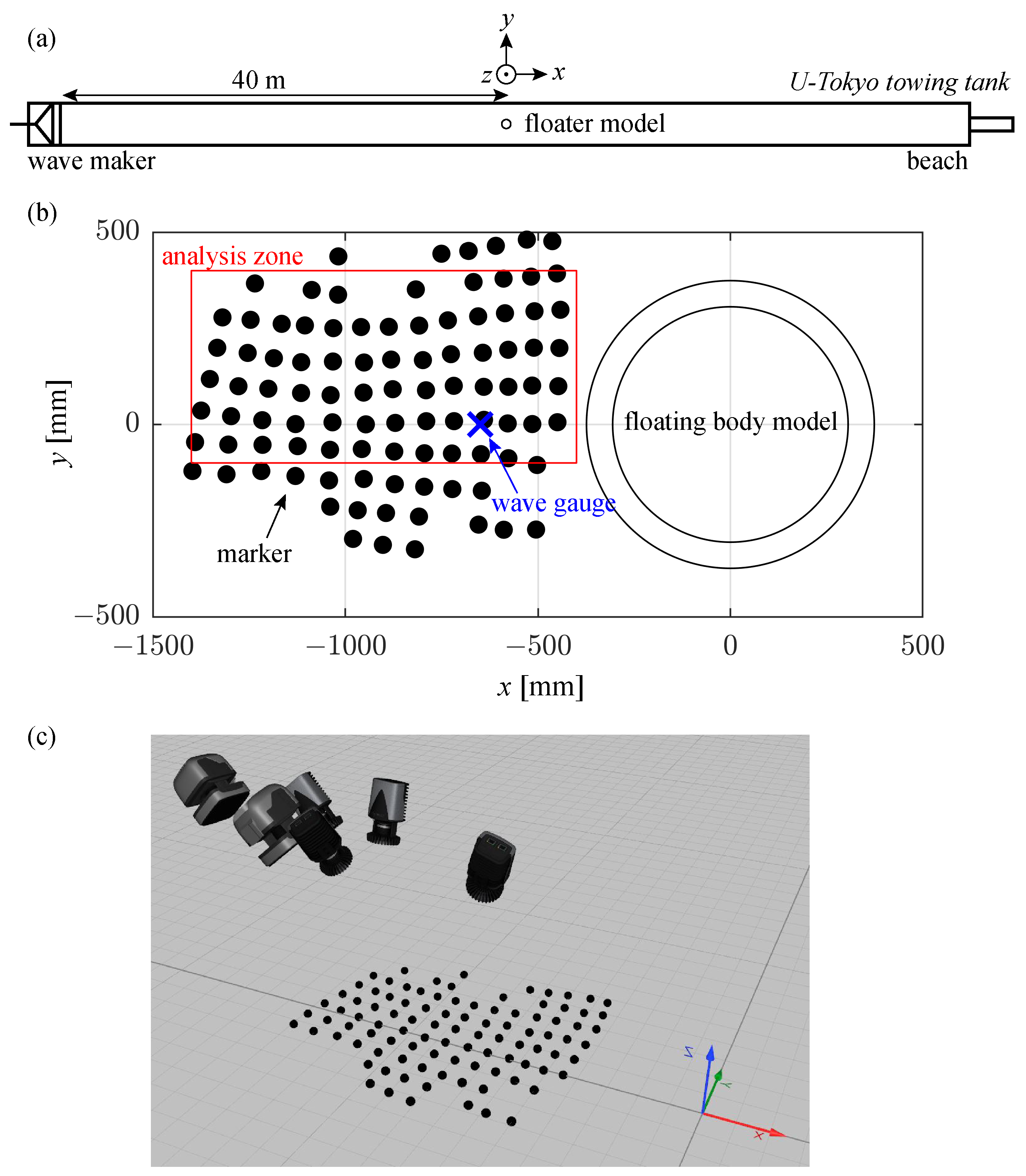
The tank experiment was performed in the towing tank (with dimensions of 85 m × 3.5 m × 2.3 m) at the University of Tokyo (Tokyo, Japan) (as illustrated in Figure 2a). A flap-type wave maker is installed at one end of this tank and a dissipation beach is installed at the other end. The floating body model was then installed at the center of the tank. The coordinate system was then defined such that coincided with the center of the model (see Figure 2b). The and z axes were set as the wave propagation direction, the transverse direction of the tank, and the vertically upward direction, respectively. Six Qualisys cameras were installed above the markers to track the 3D motion of these markers (Figure 2c). The analysis zone for the wave fields in this study was limited to the area with boundaries of mm mm and mm 400 mm, which is marked by the red rectangle in Figure 2b. By applying a TPS to the 3D coordinates of the markers (Section 2.1), the surface elevation was then evaluated in a regular grid at intervals of 10 mm within this area. A servo-controlled wave gauge (WG) was then installed at within this analysis zone, as indicated by the blue cross in Figure 2b, to validate the stereo-reconstructed wave fields obtained using the proposed method.
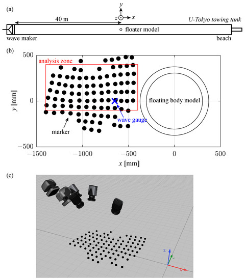
Figure 2.
Experimental setup in the towing tank. (a) Floating body model location in the towing tank (top view); (b) arrangement of the floating body model, the marker net, and the wave gauge (WG) (top view); (c) setup of the stereo cameras (SCs).
3.2. Marker Net
To enable placement of the target markers in a regular grid on the water surface, the markers were attached to a flexible net at intervals of approximately 100 mm. An image of this marker net is shown in Figure 3. Styrofoam spheres with a diameter of 10 mm were used as the target markers. 144 markers were placed on the net (in 12 rows × 12 columns), although only approximately half of the markers could be detected successfully by the SC systems. The horizontal motions of the markers were weakly constrained by attaching them to the net nodes. Each marker can be assumed to largely follow the wave surface motion because the wavelength of the waves generated during the experiment is at least 150 times longer than the marker size of 10 mm in diameter. The shortest wavelength of the regular wave generated in the tank was approximately 1.5 m, corresponding to a wave period of s (see Section 3.4). The markers were covered with retro-reflective tapes to allow the infrared Qualisys SCs to capture the infrared light reflected by the markers.
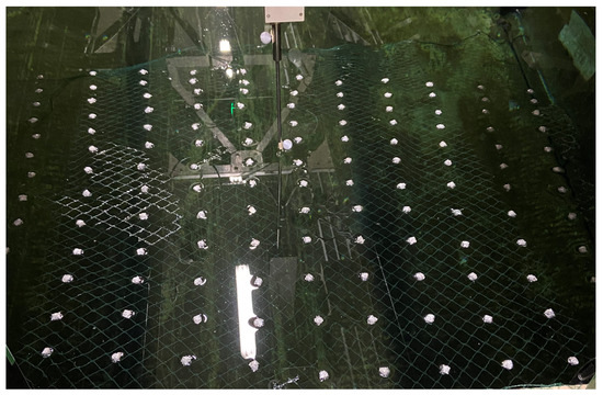
Figure 3.
Image of the marker net in the tank.
3.3. Stereo Cameras
The six Qualisys cameras (Figure 2c) comprised four Miqus (1216 × 800 pixels) cameras and two Arqus (4200 × 2160 pixels) cameras. The 3D motion of each marker was estimated based on the images acquired by these cameras using the Qualisys tracking manager (QTM) software (Qualisys AB, Göteborg, Sweden).
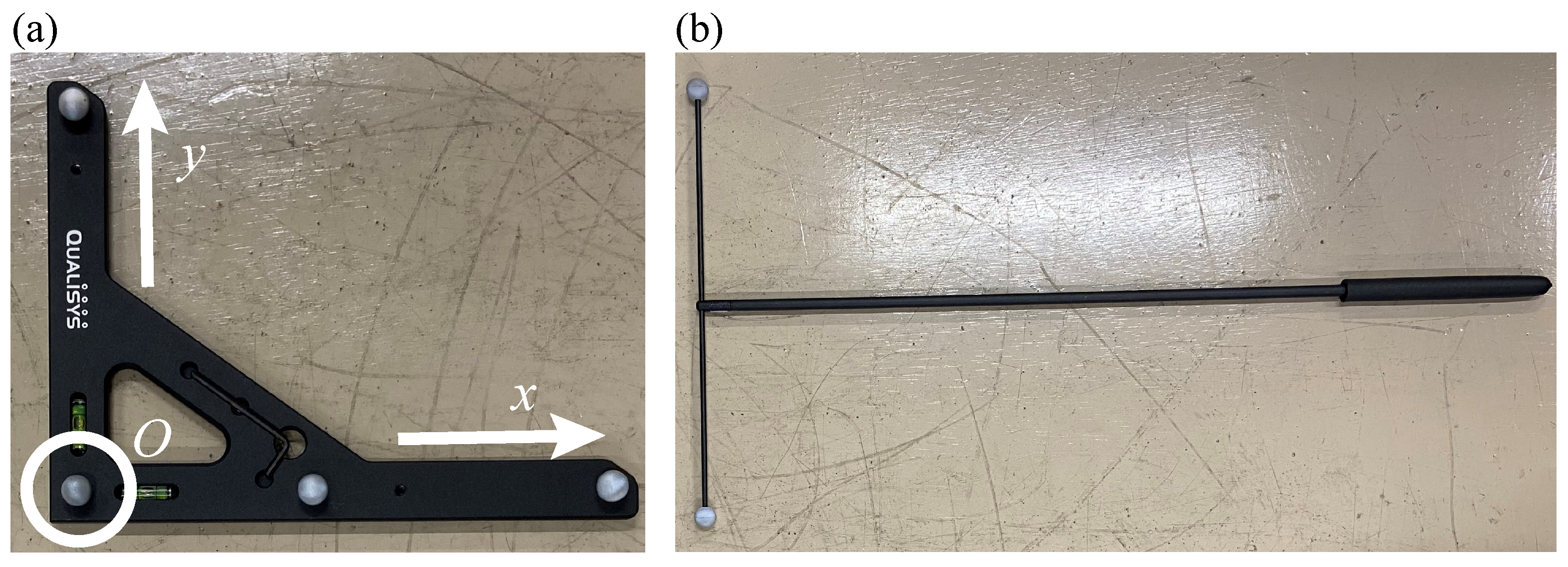
The intrinsic and extrinsic parameters of these cameras are required to evaluate the 3D coordinates of each marker [15]. The intrinsic parameters, which relate to the focal lengths and optical centers of the cameras, were calibrated prior to shipment and stored in the camera memory. The extrinsic parameters, which represent the specific positions and orientations of the cameras, were calibrated according to the QTM standard method [37] using an L-shaped reference frame and a T-shaped wand (Figure 4). Specifically, the L-shaped frame was placed within the field of view of the cameras, and the T-shaped wand was moved within the measurement volume. This calibration method defined the coordinate system for the SC system based on the L-shaped frame. The longer and shorter arms of the reference frame correspond to the x and y axes, respectively, and the z axis is orthogonal to these arms. The marker indicated by the circle represents the origin O of the coordinate system. This coordinate system was dependent on the placement of the L-shaped reference frame within the tank during the calibration process. Therefore, after calibration, the coordinate system was transformed via rotation and translation [27] to ensure that the plane coincided with the mean water surface and that coincided with the center of the floating body model (Figure 2b).
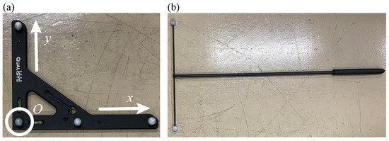
Figure 4.
SC calibration kit. (a) L-shaped reference frame. (b) T-shaped calibration wand.
3.4. Wave Conditions
Unidirectional regular waves were generated in the tank. Table 3 lists the parameters of these regular waves. To separate the scattering and radiation waves, the wave field measurements were performed under three different model constraints, designated cases (i)–(iii), as described in Section 2.2. In case (iii), experiments were also conducted without the marker net to determine whether the marker net itself affects the floating body motion and the surrounding wave fields. The floating body motion and wave elevation characteristics measured using the WG are compared under the conditions with and without the marker net in Section 5.2. The measurements under all incident wave conditions and all model constraint conditions were repeated three times. The mean and the standard deviation of results of the the three repeated measurements are presented in the following sections. Note that for the SC measurement performed under the incident wave conditions of and , only two repeated test results were analyzed.
Table 3.
Parameters of the waves generated in the towing tank.
Only three conditions for the incident wave period are insufficient to provide detailed motion characteristics of the floating body model represented by a response amplitude operator (RAO). However, the primary objective of the tank test is not to investigate motion characteristics in detail but to demonstrate the performance of the proposed stereo reconstruction method for wave fields around the model. For this purpose, it is essential to evaluate the measurement uncertainty with respect to repeatability and to demonstrate the capability to separate radiation and scattering waves from the measurement under different model constraint conditions. Therefore, given the limited duration of the experimental campaign, we prioritized performing experiments with different model constraint conditions and repeated tests over adopting a number of wave period conditions. Instead, we carefully chose the three wave periods, and 2 (s), such that this range of wave periods covers the natural periods of the heave and pitch motions of the model (1.55 s and 1.71 s, respectively) to conduct experiments under different motion characteristic conditions.
4. Results
The results of wave field reconstruction around the floating body model when using the proposed method are presented in this section. The reconstructed wave elevation at the WG position is compared with the WG record to validate the results from the proposed method. The time intervals of the analysis are selected such that the wave amplitudes measured using the WG are almost stationary. The same time intervals are selected for the same incident wave period, regardless of the model constraint conditions used (cases (i)–(iii)).
4.1. Motion Characteristics of the Floating Body Model in Waves
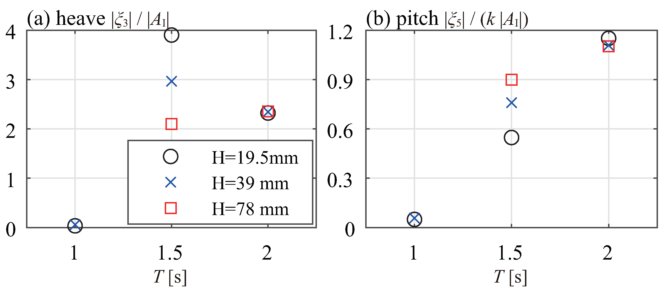
The motion responses of the floating body model to waves are examined briefly in this section. The amplitudes of the floating body motions under all wave conditions are shown in Figure 5. The heave amplitude is normalized with respect to the incident wave amplitude (case (i)) and the pitch amplitude is normalized with respect to the incident wave steepness .
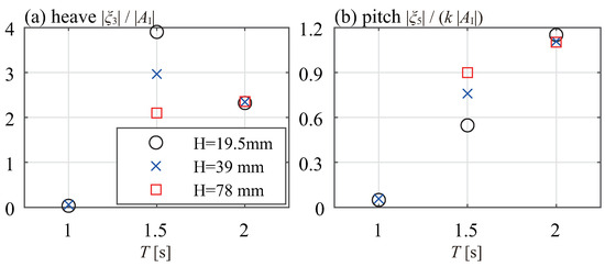
Figure 5.
Normalized amplitudes of the floating body motions. (a) Heave; (b) pitch.
Significant nonlinear heave and pitch motion characteristics with respect to the incident wave height are observed for the model at the wave period of s. The period s is approximately equal to the natural period of the heave (1.55 s) and is slightly shorter than the natural period of the pitch (1.71 s). Similar nonlinear motion characteristics were also observed in earlier studies [35,36], although the draft of the model in these cases was shallower than that of the present model. Different motion characteristics with respect to the incident wave conditions will affect the wave fields around the floating body model. The differences in the spatial wave patterns that depend on the incident wave conditions will be presented in Section 5.1.
Note that in certain cases, the transient floating body motions did not necessarily disappear during the time interval that was analyzed. Therefore, the motion amplitudes shown in Figure 5 do not necessarily represent the motions that occur in a stationary (time-harmonic) state. However, the transient motion behavior of the floating body does not represent a problem for verification of the stereo reconstruction method for the wave fields around a floating body proposed in this study. The motion amplitudes shown in Figure 5 represent the floating body motions recorded at the same time that the wave field to be reconstructed below was measured.
4.2. Validation versus Wave Gauge Records
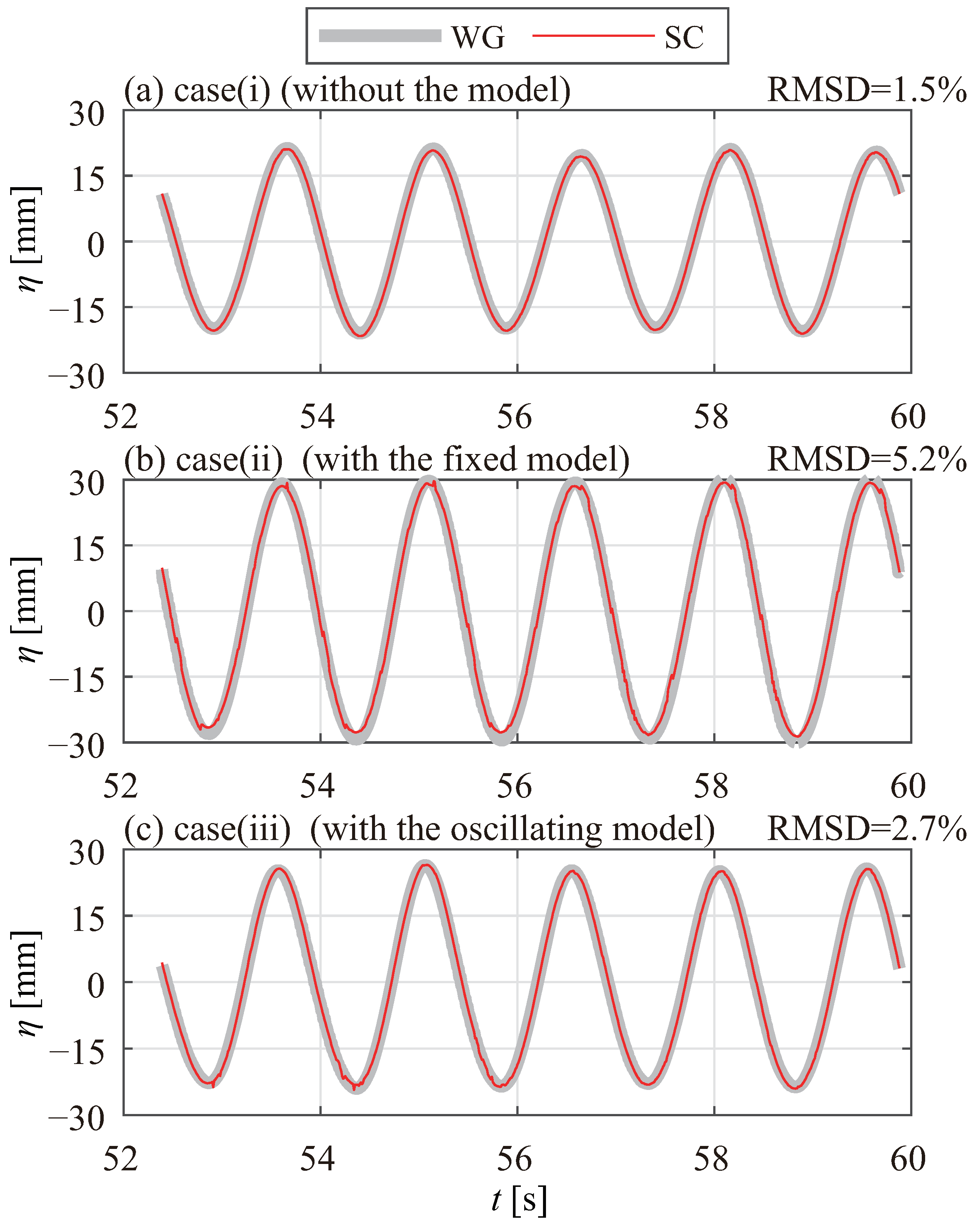
In this section, the proposed wave field reconstruction method is validated via comparison of the wave elevation time series with the WG records. The wave elevation time series measured using an SC and the WG are compared in Figure 6 under the incident wave condition characterized by s and mm. The mean values of the repeated measurements are plotted in the figure. The wave amplitudes at the WG position differ between cases (i)–(iii) because of the superposition of the scattering and radiation waves on the incident waves. The agreement between the time series of the SC and the WG appears satisfactory.
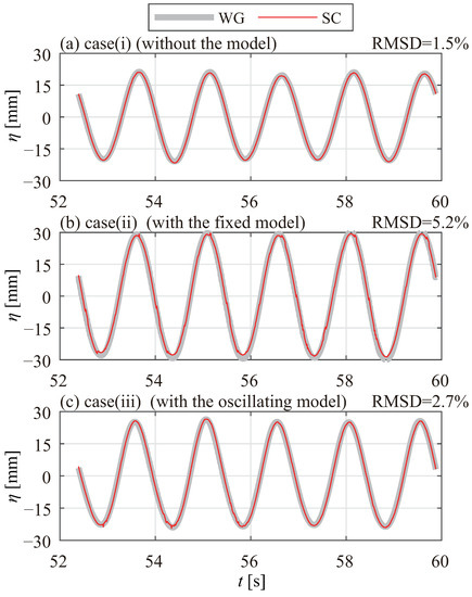
Figure 6.
Comparison of the surface elevation time series of the waves under the incident wave condition characterized by s and mm from the SC and WG measurement results. (a) Case (i); (b) case (ii); (c) case (iii).
To discuss this agreement quantitatively, the root mean square deviations (RMSDs) between the SC and WG time series ( and , respectively) were evaluated as follows:
where the subscript j denotes the time step index and N denotes the number of data used to evaluate the RMSD (corresponding to a period of , as shown in Figure 6). The is normalized with respect to the incident wave amplitude determined from the WG record. The evaluated RMSD values are noted in Figure 6 and are less than approximately 5% in all of cases (i)–(iii) under incident wave condition characterized by s and mm.
The comparison of the wave elevation between the SC and the WG here is performed at a single point. However, the SC measurement accuracy at the WG position can be considered to be representative of the accuracy throughout the analysis zone. This consideration holds because the SC measurement is independent of the floating body model. The distance that separates the wave elevation reconstruction position from the model thus does not affect the measurement accuracy. Therefore, the apparently satisfactory agreement confirmed by the RMSD values validates the proposed wave field reconstruction method using the SCs in combination with the marker net.
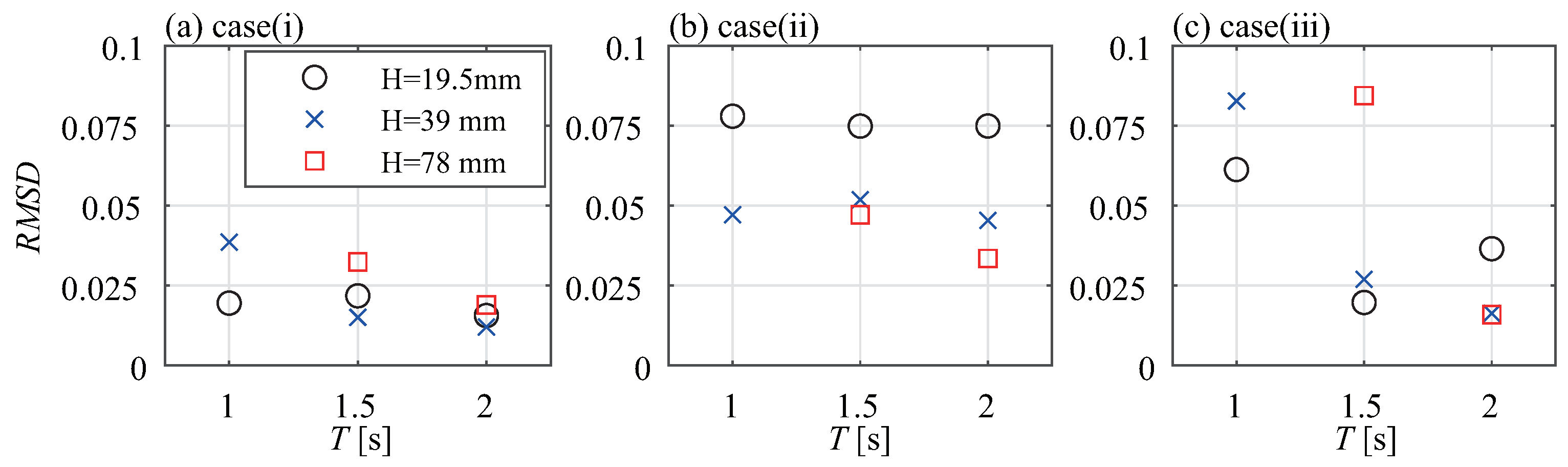
The RMSD values for all incident wave conditions and all model constraint conditions (cases (i)–(iii)) are shown in Figure 7. These RMSD values are confirmed to be less than 9% under all the above conditions. Comparison of the RMSD values among cases (i)–(iii) indicates that the difference between the SC and WG measurement results tends to be greater in the cases with the floating body model (cases (ii) and (iii)) than in the case without the model (case (i)). The larger RMSD values observed in the case with the floating body model can be explained by generation of ripples within the vicinity of the model. These ripples reflect the infrared light, which can cause degradation of the marker matching among the different camera images and thus affect the stereo reconstruction accuracy (Appendix A).
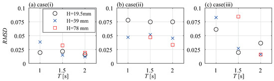
Figure 7.
Comparison of the wave elevation time series obtained from the SC and WG measurement results. (a) Case (i); (b) case (ii); (c) case (iii).
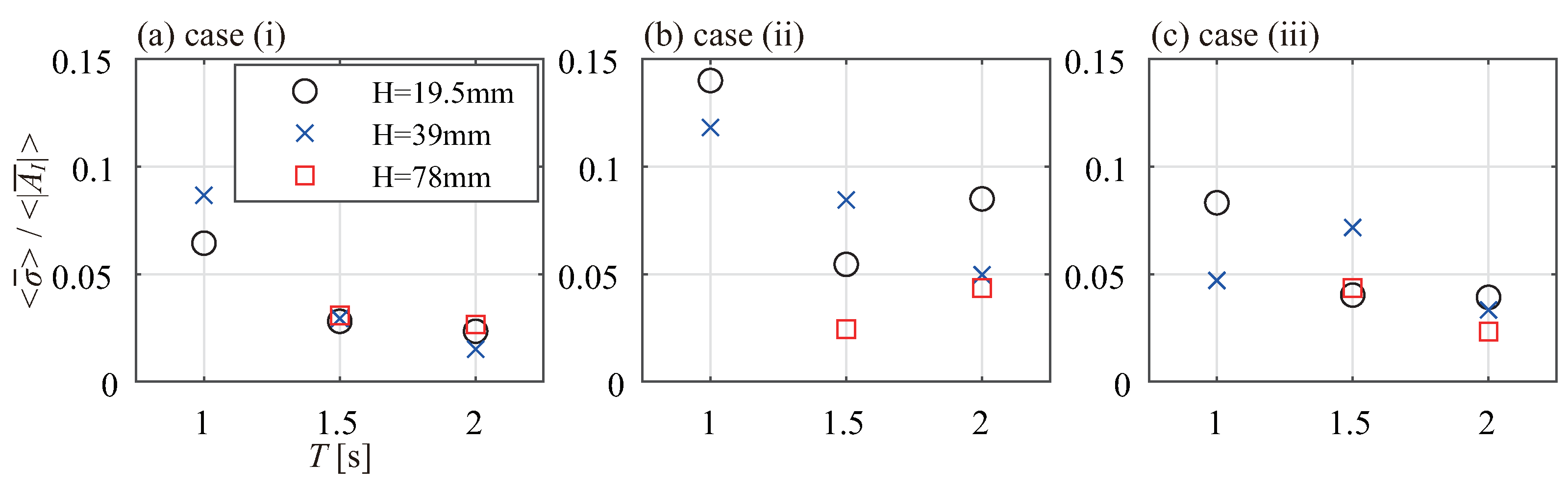
The mean values of the repeated SC measurements have been investigated. In the following, the variations in the repeated SC measurements are examined. The spatiotemporal mean of the unbiased standard deviation of the repeated SC measurements was evaluated as follows. First, the unbiased standard deviation of the repeated measurement for the wave elevation at each node within the analysis zone (Figure 2a) was evaluated. Next, its temporal mean was calculated for one wave period . Finally, its spatial mean was calculated over the analysis zone . Note that, hereafter, the angle brackets “” are used to indicate the spatial mean and the overlines “” are used to represent the temporal mean in this study.
results for all incident wave conditions and all model constraint conditions (i.e., cases (i)–(iii)) are shown in Figure 8. Under good conditions, e.g., the cases without the floating body model for incident wave periods longer than 1.5 s, the wave fields can be obtained with a variation of approximately 2–3% in the incident wave amplitude. Overall, however, the variation in the repeated measurements increases for the case with the floating body model. This behavior can also be explained by the SC measurement accuracy degradation associated with generation of ripples around the floating body model (Appendix A).
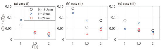
Figure 8.
Spatiotemporal mean values of the standard deviation of the repeated SC measurements of the wave elevation. (a) Case (i); (b) case (ii); (c) case (iii).
4.3. Stereo Reconstruction of Wave Fields
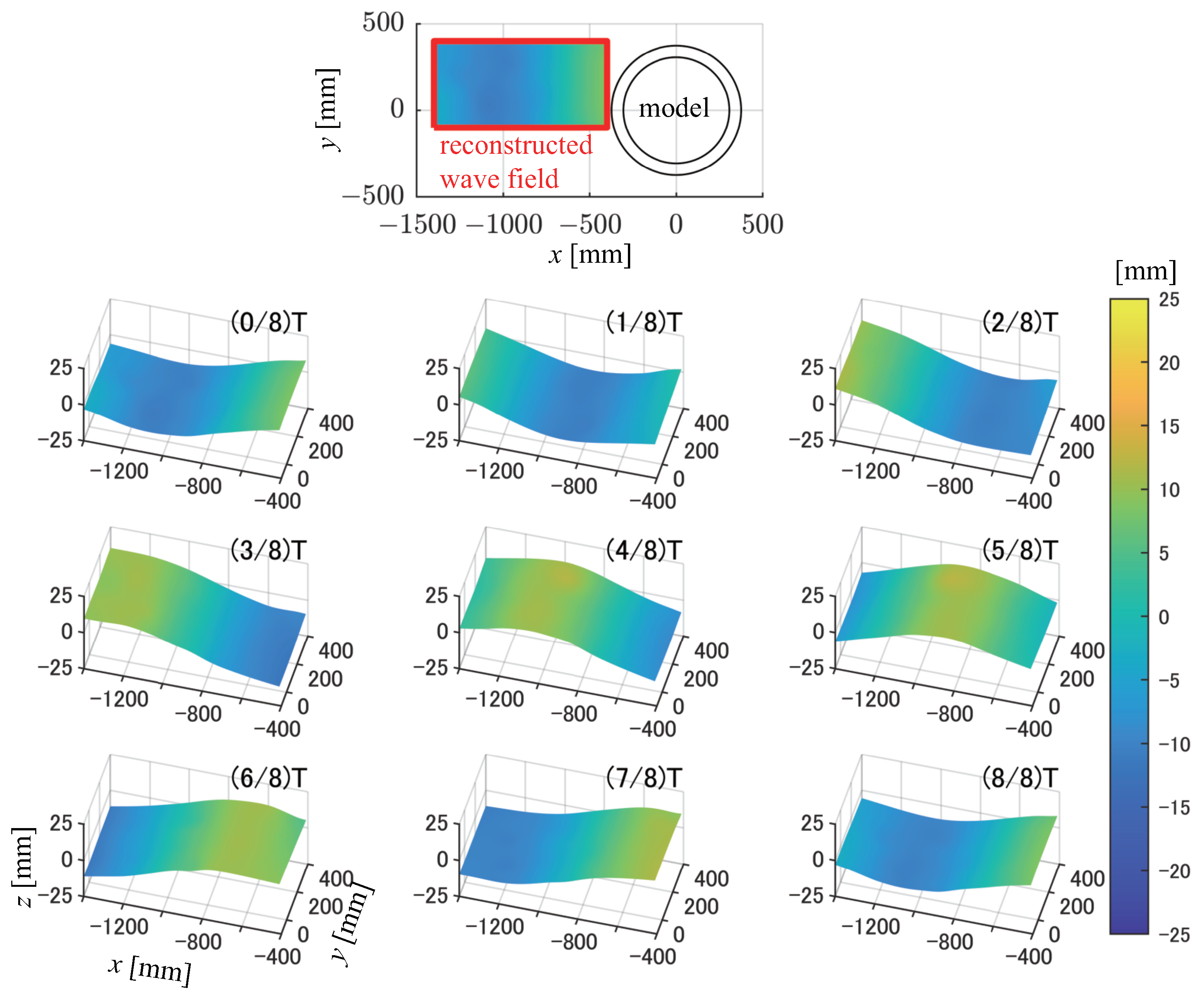
The wave elevation time series obtained using the proposed method at a single point were compared with the WG records in the previous section. In this section, the 3D surface wave profiles around the floating body model that were reconstructed using the SCs are presented while focusing on the incident wave condition characterized by s and mm for an example. Figure 9 shows the time sequence of the wave field snapshots in case (i), i.e., without the floating body model, for one wave period T at intervals of . The mean from the three repeat tests is drawn in the figure. The time is adjusted such that the first snapshot acquired at , as denoted by “” in the figure, corresponds to the time at which the incident wave crest is at . The temporal evolution of the wave fields and the qualitative coincidence of the wave fields at and T confirm that the proposed stereo imaging method can capture the following fundamental regular wave behaviors successfully: propagation in the direction and periodically over time.
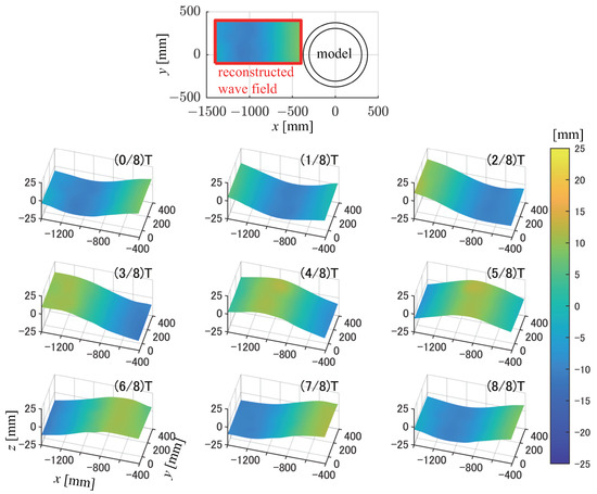
Figure 9.
Spatial profiles of an incident regular wave with s and mm. Nine snapshots acquired at intervals of T/8 within a wave period T are presented. The positional relationship between the reconstructed wave fields and the floating body model is indicated at the top of the figure.
The two spatial wave profiles at and , denoted by and in the figure, respectively, are essential to understanding of the time-harmonic behavior of the wave field. This is because the spatial wave profiles in the analysis zone can be expressed at any time using these two wave profiles under the linear wave assumption for the following reason. The time series of the wave elevation at any position around the floating body model can be expressed as the sum of the Fourier series with fundamental frequency :
with
where denotes the higher-order terms. Recall that was set when an incident wave crest was at . If the higher-order terms are ignored, then the spatial wave profiles at and can be interpreted to be expressing the amplitudes of the cosine and sine components, and , respectively, [3,4]. Therefore, the wave elevation at any time can be recovered from the spatial wave profiles determined at and using Equation (5) within the linear wave regime. In the following, the spatial wave profiles at and are considered to be and , and we focused on these profiles.
and were acquired using the SCs for cases (i)–(iii) under the incident wave condition characterized by s and mm and are compared in Figure 10. The wave amplitudes were normalized with respect to the spatial mean of the incident wave amplitude . The wave fields around the fixed model (case (ii), Figure 10b,e) and the oscillating model (case (iii), Figure 10c,f) are different to the incident wave profiles (case (i), Figure 10a,d). The wave elevations remain almost constant in the y-direction for the incident waves (case (i)) alone, while the wave elevations vary in the y-direction for the two cases in the presence of the floating body model (i.e., cases (ii) and (iii)). These wave field characteristics in cases (ii) and (iii) confirm that the SCs can capture the superposition of the scattering (or disturbance) waves on the incident waves.
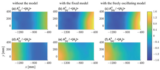
Figure 10.
Spatial profiles of the wave amplitudes under the incident wave condition characterized by s and mm. (a–c) and (d–f) represent the cosine and sine component amplitudes ( and ), respectively. (a,d), (b,e), and (c,f) show the results for the test cases (i), (ii), and (iii), respectively.
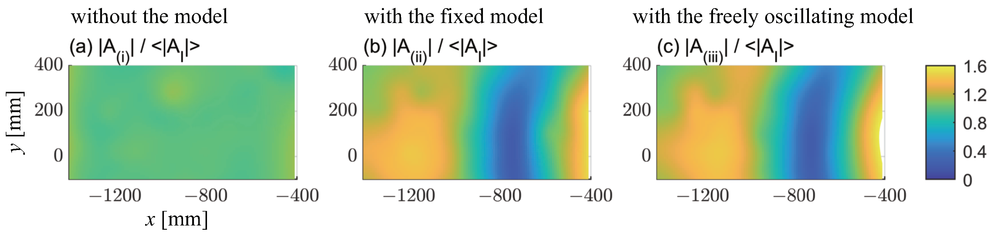
The difference between the wave fields with and without the floating body model can be seen clearly in the spatial distribution of the wave amplitude . The spatial distributions of in cases (i)–(iii) are compared in Figure 11. was calculated based on the Fourier amplitudes of the reconstructed wave elevations at each grid point within the analysis zone. As expected, remains almost constant in space in case (i), in which only the incident wave is present. In contrast, the spatial distribution of is remarkable in both cases (ii) and (iii), in which the scattering or disturbance waves coexist with the incident waves. The spatial pattern of observed in cases (ii) and (iii) implies that scattering or disturbance waves are generated cylindrically from the floating body model.

Figure 11.
Spatial profiles of wave amplitudes under the incident wave condition characterized by s and mm. (a) Case (i); (b) case (ii); (c) case (iii).
Under this incident wave condition, the spatial wave patterns in cases (ii) and (iii) appear to be similar, as indicated by the cosine and sine component amplitudes (Figure 10) and the absolute amplitude (Figure 11). The similarity of these wave patterns is attributed to the negligible floating body motions that occur in case (iii) under this wave condition (Figure 5). The negligible floating body motions that occur in case (iii) result in realization of almost the same surrounding wave field around the fixed floating body model that occur in case (ii).
5. Discussion
5.1. Extraction of Scattering and Radiation Waves
Comparison of the wave elevations from the SC and WG measurements in Section 4 showed that the proposed method using SCs in combination with marker nets could reconstruct the wave fields around a floating body model successfully. Next, as an application of the proposed method, the component waves, including the scattering wave , the radiation wave , and the disturbance wave , are extracted from the wave fields measured under the different model constraints of cases (i)–(iii). These wave field extractions are performed using the methods given in Table 1, where the mean wave fields from the repeated measurement results are used. Some examples of extracted wave fields are presented in this section.
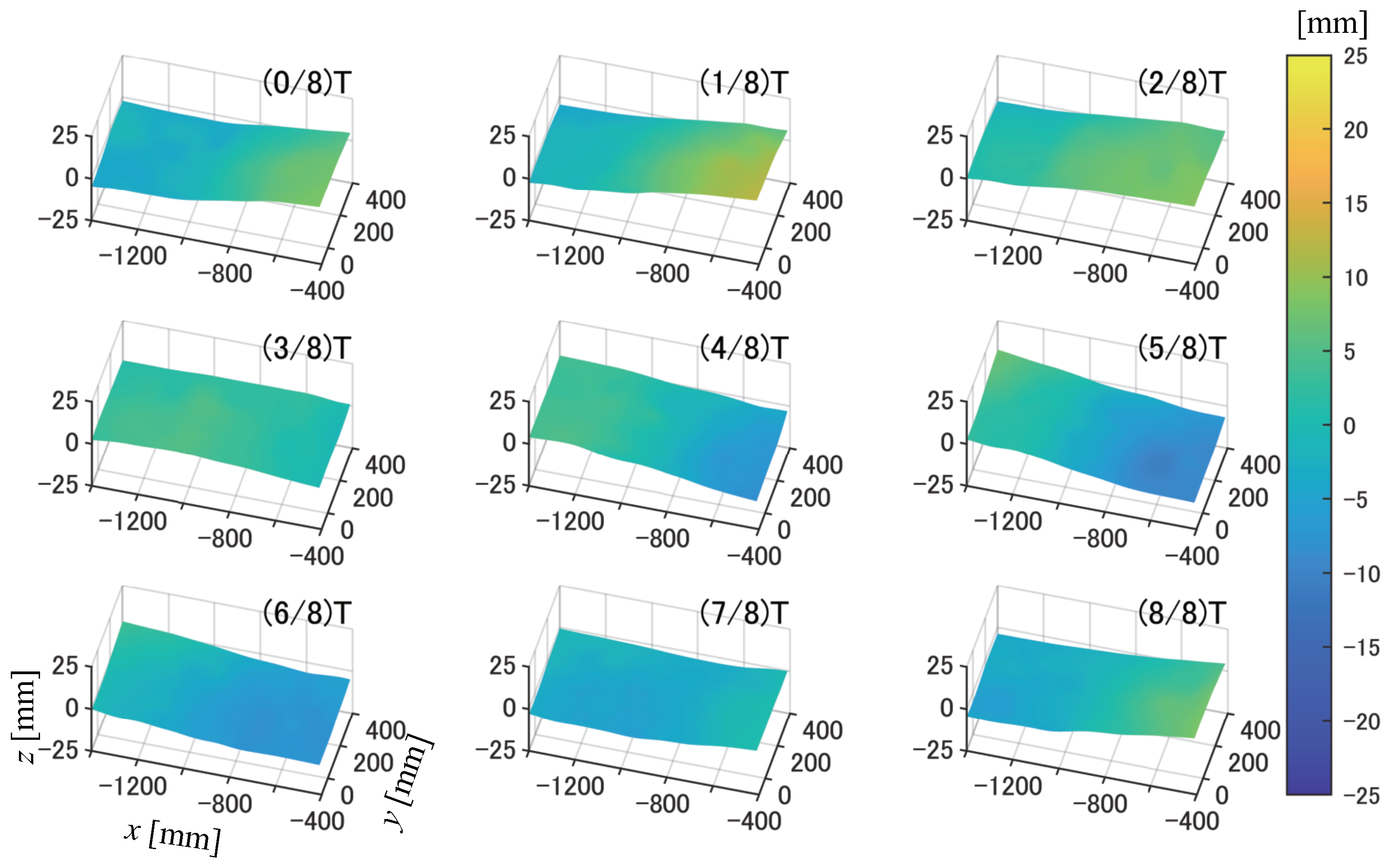
The spatial profiles of the extracted scattering wave under the incident wave condition characterized by s and mm are shown in Figure 12. The snapshots for a single wave period T are presented at intervals of at exactly the same times as the incident wave snapshots in Figure 9. In contrast to the incident wave, the scattering wave is observed to propagate away from the floating body model and mainly propagates in the direction. In addition, unlike the incident wave with its constant wave elevation in the y-direction, the horizontally two-dimensional wave elevation distribution of the scattering wave can be captured. These wave field characteristics, unlike those of the incident waves presented in Section 4.3, indicate successful extraction of the scattering wave using the method given in Table 1.
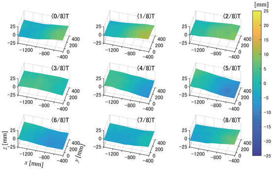
Figure 12.
Spatial profiles of a scattering wave under the incident wave condition characterized by s and mm. Nine snapshots recorded within a wave period T at intervals of T/8 are shown.
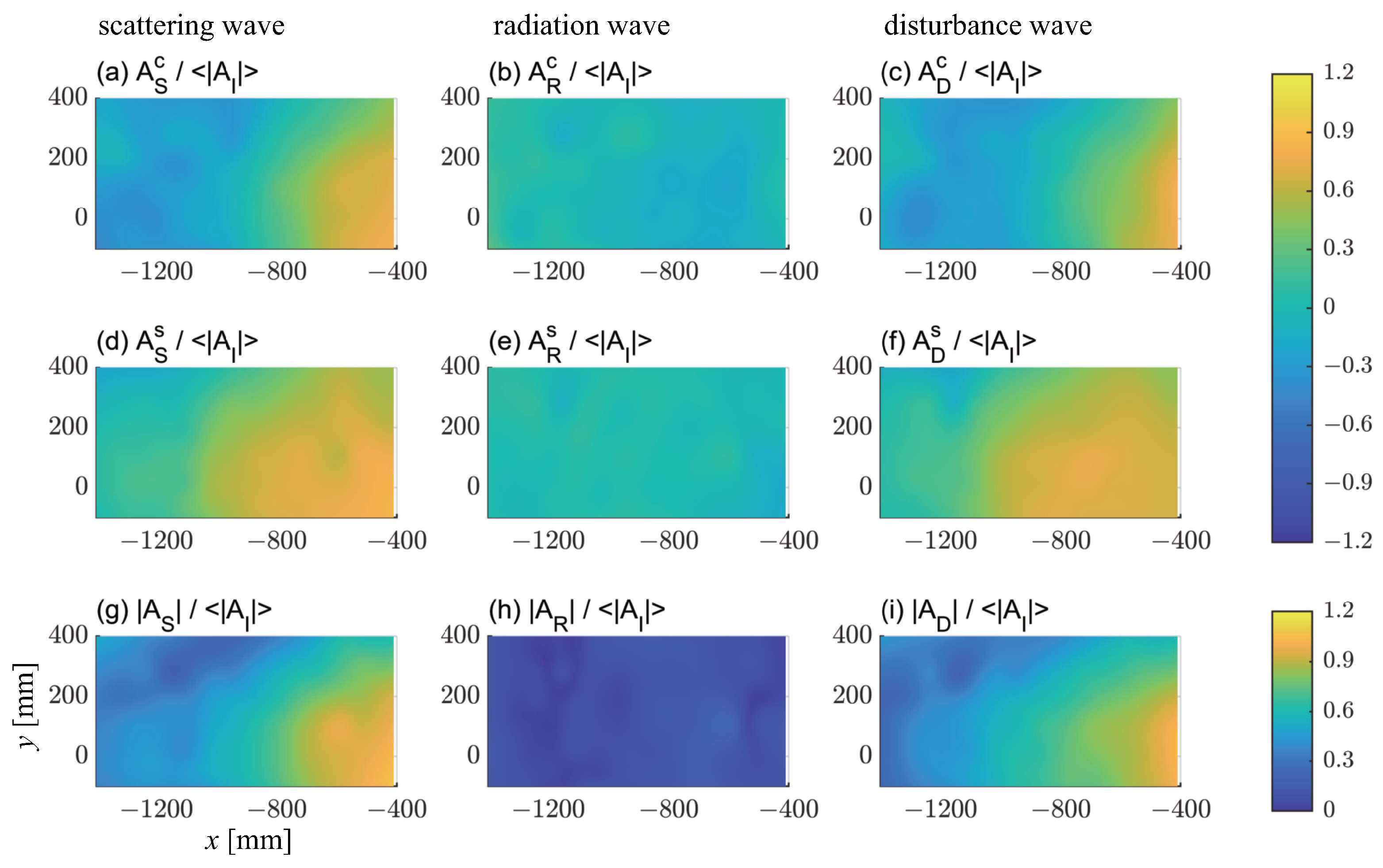
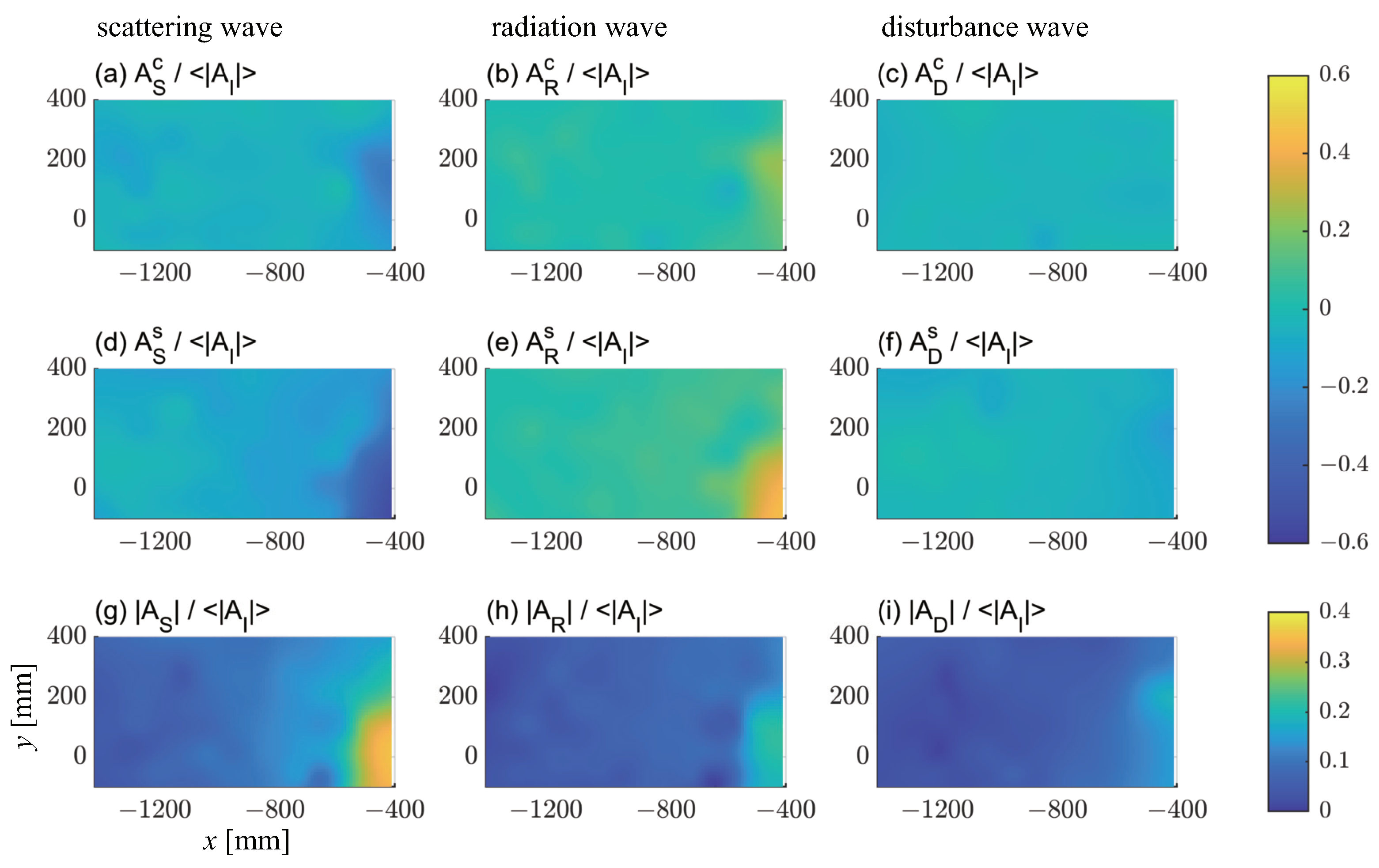
Therefore, the method described in Table 1 enables observation of the different spatial patterns of the scattering, radiation, and disturbance waves, which are dependent on the incident wave conditions. As examples, the spatial profiles of the scattering wave (), the radiation wave (), and the disturbance wave () under incident wave conditions characterized by and are presented in Figure 13 and Figure 14, respectively. The cosine and sine components of the amplitudes ( and , respectively) and the absolute amplitudes are shown in these figures.
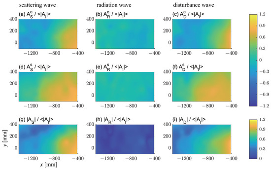
Figure 13.
Spatial profiles of the wave amplitudes under the incident wave condition characterized by s and mm. (a–c), (d–f), and (g–i) represent the cosine component, sine component, and absolute amplitudes (, , and ), respectively. (a,d,g), (b,e,h), and (c,f,i) represent the scattering waves (), the radiation waves (), and the disturbance waves (), respectively.

Figure 14.
Spatial profiles of the wave amplitudes under the incident wave condition characterized by s and mm. (a–c), (d–f), and (g–i) represent the cosine component, sine component, and absolute amplitudes (, , and ), respectively. (a,d,g), (b,e,h), and (c,f,i) represent the scattering waves (), the radiation waves (), and the disturbance waves (), respectively.
The comparison of with in Figure 13 shows that the radiation wave is much smaller than the scattering wave under the incident wave condition characterized by s and mm. The almost negligible nature of the radiation waves can be interpreted as being caused by the very small heave and pitch motions of the floating body model under this incident wave condition (Figure 5). Accordingly, the spatial patterns of and resemble each other. The above also explains the resemblance of the wave patterns around the floating body model for the motion-fixed (case (ii)) and motion-free (case (iii)) conditions under this incident wave condition, as illustrated in Figure 10 and Figure 11.
Additionally, distinct heave and pitch motions are observed under the incident wave condition characterized by s and mm (Figure 5). Therefore, in addition to the scattering wave, radiation waves attributed to the floating body motions are observed under this incident wave condition (Figure 14). Intriguingly, the spatial patterns of the scattering and radiation waves are similar but are almost opposite in phase. This leads to smaller disturbance wave amplitudes (Figure 14c,f,i) because they are given by the sum of the scattering and radiation waves. This mutual relationship among the scattering, radiation, and disturbance waves cannot be resolved by simply measuring the wave field around a freely oscillating floating body model alone. The relationship can only be obtained by measuring the wave fields under different model constraint conditions and then separating the component waves.
5.2. Influence of Marker Nets on the Surrounding Wave Field
In the previous sections, the spatial wave profiles around a floating body model were reconstructed successfully using SCs in combination with marker nets, and the scattering, radiation, and disturbance waves could then be separated from the wave fields acquired under the different model constraints. Finally, this section examines whether the marker nets affect both the floating body motions and the surrounding wave fields.
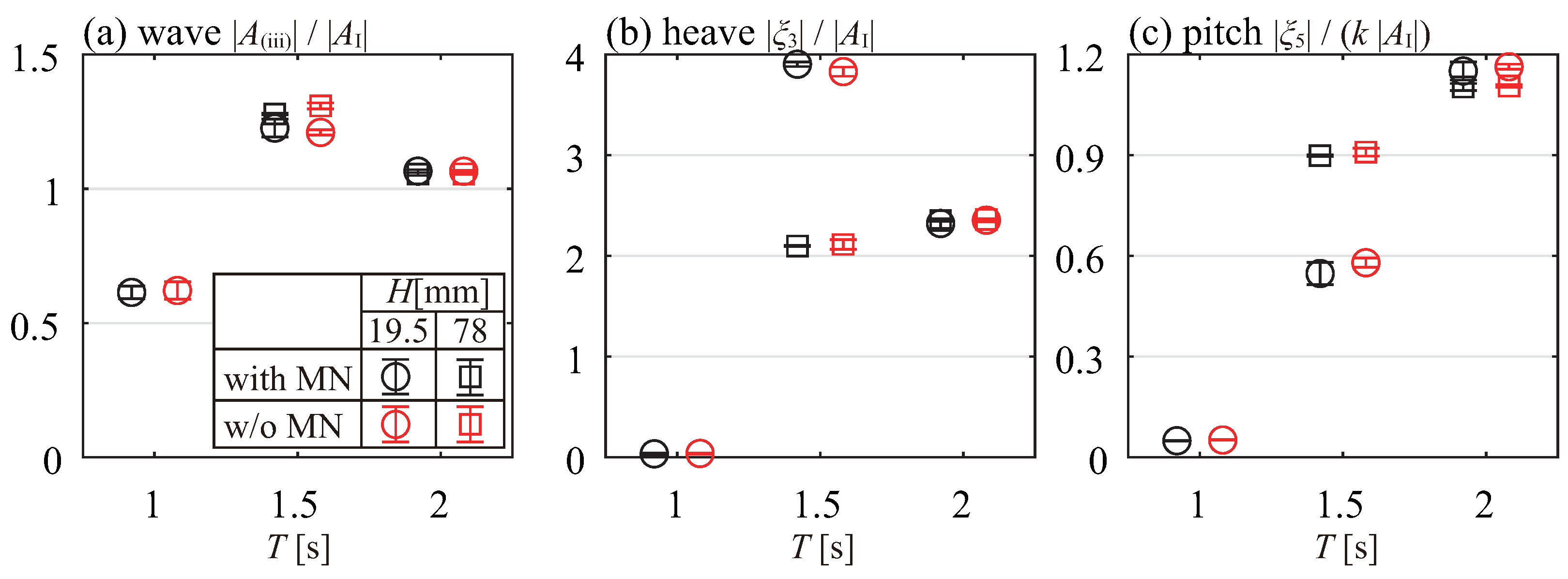
For this purpose, the floating body motions and the wave elevation at the WG position were measured under the motion-free condition (case (iii), Section 2.2) and were also measured without the marker net at the incident wave heights with mm and 78.0 mm. The normalized wave, heave, and pitch amplitudes (, and , respectively) with and without the marker net are compared in Figure 15. The means of the repeated measurement results are presented, along with error bars that express the unbiased standard deviations. The differences observed in the amplitudes of the wave, heave, and pitch with and without the marker net appear to be small under all wave conditions. Specific mean and standard deviation values are also listed in Table 4. With the exception of the incident wave condition characterized by s and mm, under which the floating body motions are particularly small, the mean amplitude differences observed between the cases with and without the marker net are mostly smaller than 2.5 %. The exception is the pitch amplitude under the incident wave condition characterized by s and mm, where the mean difference is 5.5 %.
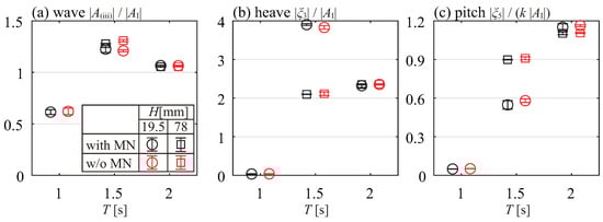
Figure 15.
Comparison of the normalized amplitudes of the wave and motion in the cases with and without the marker net. (a) Wave at the WG position; (b) heave; (c) pitch.
Table 4.
Amplitudes of the wave (at the WG position), heave, and pitch with and without the marker net, where “diff” denotes the mean amplitude difference between the cases with and without the marker net and d denotes Cohen’s d.
The mean difference values appear to be small, but this does not necessarily mean that the effect of the marker net on the motion of the floating body and its surrounding wave fields is negligible. Therefore, the magnitudes of these mean difference values relative to the representative measurement variability must be examined in the following. For this purpose, we introduce Cohen’s d, which is commonly used in statistics and expresses the mean difference standardized with respect to the representative standard deviation [38]:
Here, x denotes the samples of the wave, heave, and pitch amplitudes acquired in repeated tests. The subscripts 1 and 2 denote the cases with and without the marker net, respectively, and represents the mean amplitude. S expresses the pooled standard deviation of samples and :
where s and n denote the unbiased standard deviation and the sample size, respectively. in Equation (7) is the bias correction term and is defined as
where denotes the gamma function. denotes the degree of freedom and is calculated as follows:
Therefore, d in this study is regarded as the magnitude of the mean amplitude difference relative to the variations that were attributed to the repeated measurements. Note that the pooled standard deviation (Equation (8)) assumes that the variances are the same between the two samples, although this assumption may not necessarily hold between measurements taken with and without the marker net.
The evaluated d values are also given in Table 4 and show that the mean differences among the amplitudes of the wave, heave, and pitch are smaller than for all incident wave conditions. Even in the cases where the mean differences are greater than 4%, e.g., the heave and pitch amplitudes for and the pitch amplitudes for , the mean differences still do not exceed . These results show that the mean differences in the amplitudes of the wave, heave, and pitch in the cases with and without the marker net are small when compared with the variability attributed to the repeated measurements. Note that an increase in the number of repeat tests may lead to a reduction in the standard deviation and an increase in d. However, based on the small values of d that were evaluated in this section, we can conclude that, in a practical sense at least, the effect of the marker net is negligible.
6. Conclusions
In this study, an experimental method for stereo reconstruction of 3D surface wave fields around floating body models in a tank was developed. The key to the success of the proposed method was the use of a marker net, in which target markers for the SCs were attached to a flexible net, to give the water surface in the tank a Lambertian characteristic. The introduction of the marker net overcame the highly specular characteristic of the water surface, which was inappropriate for stereo imaging techniques. The proposed method was validated via comparison with servo-controlled WG recordings.
Errors and variations in the measurement of 3D wave fields were carefully evaluated. One source of these measurement errors or variations is infrared light reflected from the ripples generated by the floating body model, because infrared cameras are used in this study. The measurement accuracy could be improved by introducing visible light cameras in combination with a suitable marker tracking system, which would require further development.
One of the notable applications of the proposed method is the 3D reconstruction of scattering and radiation wave fields generated by floating body models. These fields have been successfully acquired from the wave fields measured under three different conditions, i.e., without the floating body model, with the fixed model, and with the freely oscillating model. The direct measurement of these fields by the proposed method can be used to investigate the nonlinearity of the system with respect to waves and floating bodies by comparing them with corresponding numerical simulations based on linear potential theory.
Author Contributions
Conceptualization, Y.H., H.H., Y.Y., S.H., H.S. and H.O.; methodology, Y.H., H.H. and Y.Y.; software, Y.H. and H.H.; validation, Y.H. and H.H.; formal analysis, Y.H. and H.H.; investigation, Y.H. and H.H.; resources, H.H. and H.S.; data curation, Y.H.; writing—original draft preparation, Y.H. and H.H.; writing—review and editing, H.H., R.T.G., Y.Y., S.H., H.S. and H.O.; visualization, Y.H. and H.H.; supervision, H.H., R.T.G. and H.S.; project administration, H.H.; funding acquisition, H.O., S.H., H.S., Y.Y. and H.H. All authors have read and agreed to the published version of the manuscript.
Funding
This research was carried out within a joint research project between the University of Tokyo and Japan Marine United Corporation and was funded by Japan Marine United Corporation. H.H. acknowledges support from JSPS KAKENHI, grant numbers 21H01538 and 22H01136.
Institutional Review Board Statement
Not applicable.
Informed Consent Statement
Not applicable.
Data Availability Statement
The data are available upon request.
Acknowledgments
We thank Takayoshi Kato and Yining He for their assistance in performing the tank experiments. We thank David MacDonald from Edanz (https://jp.edanz.com/ac) (accessed on 25 August 2023) for editing a draft of this manuscript.
Conflicts of Interest
The authors declare no conflict of interest.
Abbreviations
The following abbreviations are used in this manuscript:
| SC | Stereo camera |
| PTV | Particle tracking velocimetry |
| TPS | Thin plate spline |
| QTM | Qualisys tracking manager |
| WG | Wave gauge |
| RAO | Response amplitude operator |
| RMSD | Root mean square deviation |
Appendix A. Sources of Error in Stereo Camera Measurements
Comparison of the wave elevations in the SC and WG measurements indicates that the SC measurement error tends to be greater because of the presence of the floating body models (Figure 7, Section 4.2). To investigate the source of the SC measurement error, the wave elevation time series measured using the SCs at the WG position under the wave condition characterized by s and mm in case (iii), where the maximum RMSD between the SC and WG measurements was observed, is presented in Figure A1. Three repeat measurement results (#1–#3) are presented, and the mean of the WG measurement results is also presented for comparison. Spikes and shifts in the wave elevations are observed in the SC measurements, particularly in #2 and #3.

Figure A1.
Wave elevation time series for the incident wave condition characterized by s and mm in the three measurements in case (iii).
Figure A1.
Wave elevation time series for the incident wave condition characterized by s and mm in the three measurements in case (iii).
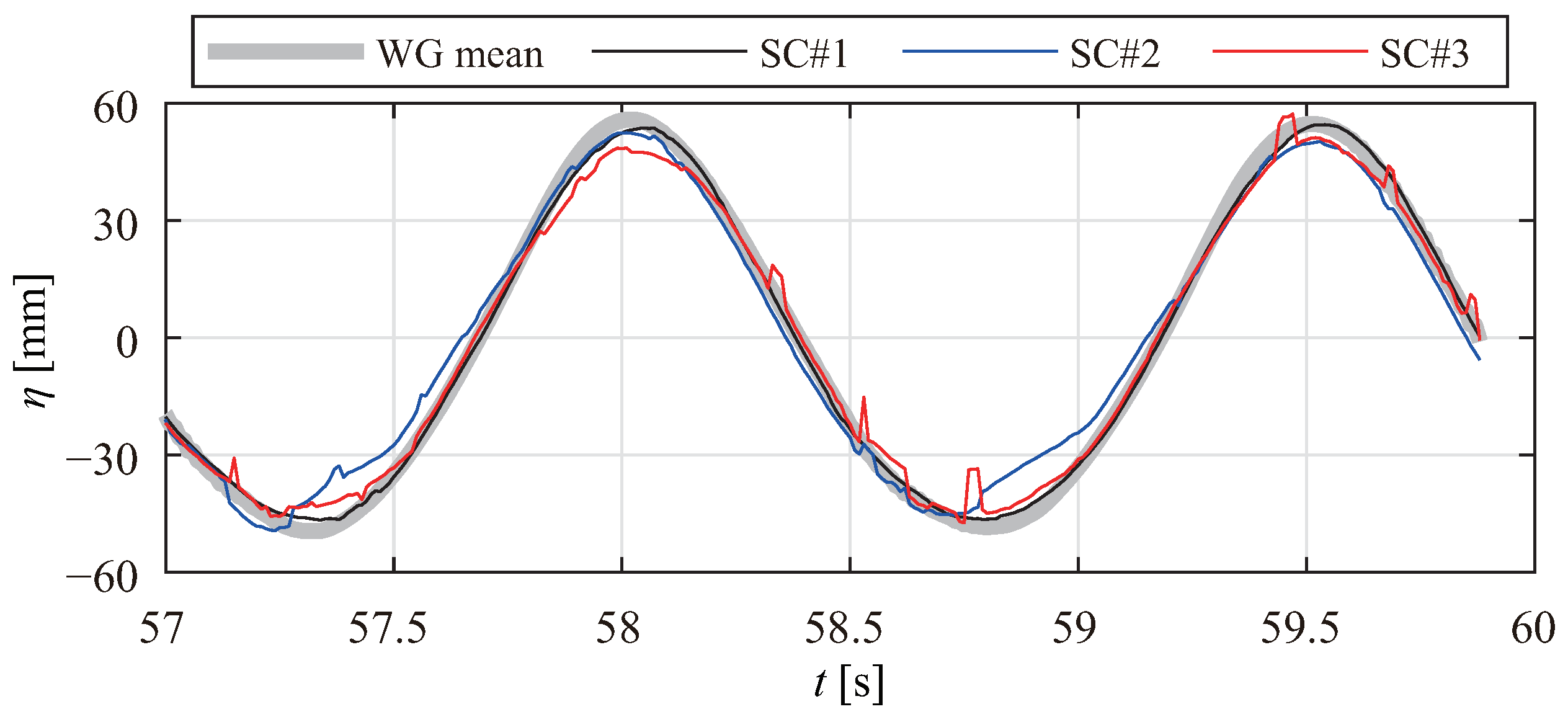
Scrutinization of the original Qualisys data revealed that the jumps in the wave elevation values were caused when the number of cameras that detected individual markers changed. One of the main causes of these changes in the number of cameras is the generation of ripples. Ripple generation was observed in the vicinity of the floating body models. These ripples reflect infrared light and the SCs then detect the light. This excess infrared light degrades the matching accuracy for the same marker among the different camera images. Accordingly, the number of cameras that detect individual markers may also change.
Therefore, the problem is not that the individual markers escape from the field of view of each camera, but that the marker matching accuracy is degraded by detection of the excess infrared light. The marker-matching algorithm is built into the QTM software and cannot be modified by the user. One possible solution to this problem is to use visible light (general) cameras for marker detection, which was performed successfully in [28].
References
- Inui, T. From bulbous bow to free-surface shock wave—Trends of 20 years’ research on ship waves at the Tokyo University Tank. J. Ship Res. 1981, 25, 147–180. [Google Scholar] [CrossRef]
- Maruo, H. Wave resistance of a ship in regular head seas. Bull. Fac. Eng. Yokohama Natl. Univ. 1960, 9, 73–91. [Google Scholar]
- Ohkusu, M. Analysis of Waves Generated by a Ship Oscillating and Running on a Calm Water with Forward Velocity. J. Soc. Nav. Archit. Jpn. 1977, 1977, 36–44. (In Japanese) [Google Scholar] [CrossRef] [PubMed]
- Kashiwagi, M. Hydrodynamic study on added resistance using unsteady wave analysis. J. Ship Res. 2013, 57, 220–240. [Google Scholar]
- Sakurada, A.; Tsujimoto, M.; Yokota, S. Application of energy saving bow shape in actual seas to JBC. In Proceedings of the International Conference on Offshore Mechanics and Arctic Engineering, American Society of Mechanical Engineers, Virtual, 21–30 June 2021; Volume 85161, p. V006T06A017. [Google Scholar]
- Maruo, H. The drift of a body floating on waves. J. Ship Res. 1960, 4, 1–10. [Google Scholar]
- Newman, J.N. The drift force and moment on ships in waves. J. Ship Res. 1967, 11, 51–60. [Google Scholar] [CrossRef]
- The Specialist Committee on Detailed Flow Measurements. Final Report and Recommendations to the 26th ITTC. In Proceedings of the 26th International Towing Tank Conference, Rio de Janeiro, Brazil, 28 August–3 September 2011; Volume II, pp. 575–625.
- Maeda, K.; Hosotani, N.; Tamura, K.; Ando, H. Wave making properties of circular basin. In Proceedings of the 2004 International Symposium on Underwater Technology (IEEE Cat. No. 04EX869), IEEE, Taipei, Taiwan, 20–23 April 2004; pp. 349–354. [Google Scholar]
- Gyongy, I.; Richon, J.B.; Bruce, T.; Bryden, I. Validation of a hydrodynamic model for a curved, multi-paddle wave tank. Appl. Ocean. Res. 2014, 44, 39–52. [Google Scholar] [CrossRef]
- Ota, D.; Houtani, H.; Sawada, H.; Taguchi, H. Optimization of segmented wave-maker control to generate spatially uniform regular waves in a rounded-rectangular wave basin. In Proceedings of the International Conference on Offshore Mechanics and Arctic Engineering. American Society of Mechanical Engineers, Virtual, 21–30 June 2021; Volume 85161, p. V006T06A064. [Google Scholar]
- Wanek, J.M.; Wu, C.H. Automated trinocular stereo imaging system for three-dimensional surface wave measurements. Ocean Eng. 2006, 33, 723–747. [Google Scholar] [CrossRef]
- Benetazzo, A. Measurements of short water waves using stereo matched image sequences. Coast. Eng. 2006, 53, 1013–1032. [Google Scholar] [CrossRef]
- Benetazzo, A.; Fedele, F.; Gallego, G.; Shih, P.C.; Yezzi, A. Offshore stereo measurements of gravity waves. Coast. Eng. 2012, 64, 127–138. [Google Scholar] [CrossRef]
- Bergamasco, F.; Torsello, A.; Sclavo, M.; Barbariol, F.; Benetazzo, A. WASS: An open-source pipeline for 3D stereo reconstruction of ocean waves. Comput. Geosci. 2017, 107, 28–36. [Google Scholar] [CrossRef]
- Lavieri, R.S.; Tannuri, E.A.; de Mello, P.C. Image-based measurement system for regular waves in an offshore basin. J. Braz. Soc. Mech. Sci. Eng. 2020, 42, 1–17. [Google Scholar] [CrossRef]
- Takahei, T.; Inui, T. The Wave-Cancelling Effects of Waveless Bulb on the High Speed Passenger Coaster M/S “KURENAI MARU” Part III-Photogrammetrical Observations of Ship Waves. J. Zosen Kiokai 1961, 1961, 105–118. (In Japanese) [Google Scholar] [CrossRef]
- Chatellier, L.; Jarny, S.; Gibouin, F.; David, L. A parametric PIV/DIC method for the measurement of free surface flows. Exp. Fluids 2013, 54, 1–15. [Google Scholar] [CrossRef]
- Gomit, G.; Rousseaux, G.; Chatellier, L.; Calluaud, D.; David, L. Spectral analysis of ship waves in deep water from accurate measurements of the free surface elevation by optical methods. Phys. Fluids 2014, 26, 122101. [Google Scholar] [CrossRef]
- Cang, Y.; He, H.; Qiao, Y. Measuring the wave height based on binocular cameras. Sensors 2019, 19, 1338. [Google Scholar] [CrossRef]
- Gomit, G.; Chatellier, L.; Calluaud, D.; David, L.; Fréchou, D.; Boucheron, R.; Perelman, O.; Hubert, C. Large-scale free surface measurement for the analysis of ship waves in a towing tank. Exp. Fluids 2015, 56, 1–13. [Google Scholar] [CrossRef]
- Tulin, M.P.; Landrini, M. Breaking waves in the ocean and around ships. In Proceedings of the Twenty-Third Symposium on Naval Hydrodynamics Office of Naval Research Bassin d’Essais des Carenes National Research Council, Val de Reuil, France, 17–22 September 2001. [Google Scholar]
- Hoyer, K.; Tulin, M.P. A stereo video imaging system for surface particle tracking. In Proceedings of the International Symposium on PIV and Modelling Water Wave Phenomena, Cambridge, UK, 17–19 April 2002. [Google Scholar]
- Waseda, T.; Sinchi, M.; Kiyomatsu, K.; Nishida, T.; Takahashi, S.; Asaumi, S.; Kawai, Y.; Tamura, H.; Miyazawa, Y. Deep water observations of extreme waves with moored and free GPS buoys. Ocean Dyn. 2014, 64, 1269–1280. [Google Scholar] [CrossRef]
- Fujarra, A.; Gonçalves, R.; Fonseca, R.; Siewert, K.; Martins, J. Optical motion capture as a techinique for measuring the water wave elevation. In Proceedings of the 4th International Workshop pn Applied Offshore Hydrodynamics (IWAOH), Rio de Janeiro, Brazil, 2–4 December 2009. [Google Scholar]
- Bispo, I.; Amouzadrad, P.; Mohapatra, S.; Soares, C.G. Motion analysis of a floating horizontal set of interconnected plates based on computer vision target tracking technique. In Advances in the Analysis and Design of Marine Structures; CRC Press: Boca Raton, FL, USA, 2023; pp. 153–159. [Google Scholar]
- Houtani, H.; Waseda, T.; Tanizawa, K. Measurement of spatial wave profiles and particle velocities on a wave surface by stereo imaging–validation with unidirectional regular waves. J. Jpn. Soc. Nav. Archit. Ocean Eng. 2017, 25, 93–102. (In Japanese) [Google Scholar]
- Mozumi, K.; Waseda, T.; Chabchoub, A. 3D stereo imaging of abnormal waves in a wave basin. In Proceedings of the International Conference on Offshore Mechanics and Arctic Engineering. American Society of Mechanical Engineers, St. John’s, NL, Canada, 31 May–5 June 2015; Volume 56499, p. V003T02A027. [Google Scholar]
- Houtani, H.; Waseda, T.; Tanizawa, K.; Sawada, H. Temporal variation of modulated-wave-train geometries and their influence on vertical bending moments of a container ship. Appl. Ocean Res. 2019, 86, 128–140. [Google Scholar] [CrossRef]
- Houtani, H.; Sawada, H.; Waseda, T. Phase convergence and crest enhancement of modulated wave trains. Fluids 2022, 7, 275. [Google Scholar] [CrossRef]
- Chabchoub, A.; Mozumi, K.; Hoffmann, N.; Babanin, A.V.; Toffoli, A.; Steer, J.N.; van den Bremer, T.S.; Akhmediev, N.; Onorato, M.; Waseda, T. Directional soliton and breather beams. Proc. Natl. Acad. Sci. USA 2019, 116, 9759–9763. [Google Scholar] [CrossRef] [PubMed]
- He, Y.; Hirabayashi, S.; Tabeta, S.; Imai, M.; Yamashita, Y. Experiment study of aircushion-type platform with simplified models and the measurement of inner wave fields. In Proceedings of the Conference Proceedings the Japan Society of Naval Architects and Ocean Engineers 35 The Japan Society of Naval Architects and Ocean Engineers, Hyogo, Japan, 17–18 November 2022; pp. 531–534. [Google Scholar]
- The MathWorks, Inc. Tpaps, Thin-Plate Smoothing Spline. Available online: https://www.mathworks.com/help/curvefit/tpaps.html (accessed on 6 July 2023).
- Xu, B.; Guyenne, P. Nonlinear simulation of wave group attenuation due to scattering in broken floe fields. Ocean Model. 2023, 181, 102139. [Google Scholar] [CrossRef]
- Suzuki, H.; Sakai, Y.; Yoshimura, Y.; Houtani, H.; Carmo, L.H.; Yoshimoto, H.; Kamizawa, K.; Gonçalves, R.T. Non-linear motion characteristics of a shallow draft cylindrical barge type floater for a FOWT in waves. J. Mar. Sci. Eng. 2021, 9, 56. [Google Scholar] [CrossRef]
- Katafuchi, M.; Suzuki, H.; Higuchi, Y.; Houtani, H.; Malta, E.B.; Gonçalves, R.T. Wave Response of a Monocolumn Platform with a Skirt Using CFD and Experimental Approaches. J. Mar. Sci. Eng. 2022, 10, 1276. [Google Scholar] [CrossRef]
- Qualisys, A.B. QTM Qualisys Track Manager User Manual; Qualisys AB: Göteborg, Sweden, 2011. [Google Scholar]
- The MathWorks, Inc. meanEffectSize, One-Sample or Two-Sample Effect Size Computations. Available online: https://www.mathworks.com/help/stats/meaneffectsize.html (accessed on 15 July 2023).


Disclaimer/Publisher’s Note: The statements, opinions and data contained in all publications are solely those of the individual author(s) and contributor(s) and not of MDPI and/or the editor(s). MDPI and/or the editor(s) disclaim responsibility for any injury to people or property resulting from any ideas, methods, instructions or products referred to in the content. |
© 2023 by the authors. Licensee MDPI, Basel, Switzerland. This article is an open access article distributed under the terms and conditions of the Creative Commons Attribution (CC BY) license (https://creativecommons.org/licenses/by/4.0/).